Phenomenology of Maximal and Near–Maximal Lepton Mixing

The possible existence of maximal or near–maximal lepton mixing constitutes an intriguing challenge for fundamental theories of flavour. We study the phenomenological consequences of maximal and near–maximal mixing of the electron neutrino with other ($x$=tau and/or muon) neutrinos. We describe the deviations from maximal mixing in terms of a parameter $\epsilon\equiv 1-2\sin^{2}\theta_{ex}$ and quantify the present experimental status for $|\epsilon|<0.3$. We show that both probabilities and observables depend on $\epsilon$ quadratically when effects are due to vacuum oscillations and they depend on $\epsilon$ linearly if matter effects dominate. The most important information on $\nu_{e}$–mixing comes from solar neutrino experiments. We find that the global analysis of solar neutrino data allows maximal mixing with confidence level better than 99% for $10^{-8}$ eV${}^{2}\mathrel{\hbox to0.0pt{\lower 4.0pt\hbox{\hskip 1.0pt$\sim$}\hss}\raise 1.0pt\hbox{$<$}}\Delta m^{2}\mathrel{\hbox to0.0pt{\lower 4.0pt\hbox{\hskip 1.0pt$\sim$}\hss}\raise 1.0pt\hbox{$<$}}2\times 10^{-7}$ eV². In the mass ranges $\Delta m^{2}\mathrel{\hbox to0.0pt{\lower 4.0pt\hbox{\hskip 1.0pt$\sim$}\hss}\raise 1.0pt\hbox{$>$}}1.5\times 10^{-5}$ eV² and $4\times 10^{-10}$ eV${}^{2}\mathrel{\hbox to0.0pt{\lower 4.0pt\hbox{\hskip 1.0pt$\sim$}\hss}\raise 1.0pt\hbox{$<$}}\Delta m^{2}\mathrel{\hbox to0.0pt{\lower 4.0pt\hbox{\hskip 1.0pt$\sim$}\hss}\raise 1.0pt\hbox{$<$}}2\times 10^{-7}$ eV² the full interval $|\epsilon|<0.3$ is allowed within $\sim$ 4$\sigma$ (99.995 % CL). We suggest ways to measure $\epsilon$ in future experiments. The observable that is most sensitive to $\epsilon$ is the rate [NC]/[CC] in combination with the Day–Night asymmetry in the SNO detector. With theoretical and statistical uncertainties, the expected accuracy after 5 years is $\Delta\epsilon\sim 0.07$. We also discuss the effects of maximal and near–maximal $\nu_{e}$-mixing in atmospheric neutrinos, supernova neutrinos, and neutrinoless double beta decay.

I Introduction

The data from both atmospheric and solar neutrino experiments have given a rather convincing evidence for non-zero neutrino masses and mixing. Furthermore, some features of the neutrino flavour parameters are surprising and quite different from the quark flavour parameters. In particular, one or two of the three mixing angles in the MNS (Maki-Nakagawa-Sakata) mixing matrix for leptons [1] are large. Specifically, the simplest interpretation of the atmospheric neutrino measurements gives [2, 3]

$$\sin^{2}2\theta_{\mu\tau}\sim 0.8-1,\,\;\;\;\;\;\Delta m^{2}_{32}\sim(2-5)\times 10^{-3}\,\mbox{\rm eV}^{2}.$$ (1)

There exist several solutions of the solar neutrino problem involving oscillations of electron neutrinos into some combination, $\nu_{x}$, of $\mu-$ and $\tau-$neutrinos with large mixing angle [4, 5, 6, 7, 8, 9, 10] with parameters in the range

$$\sin^{2}2\theta_{ex}\sim 0.7-1,\,\;\;\;\Delta m^{2}_{12}\sim(0.2-4)\times 10^{-4}\,\mbox{\rm eV}^{2}\;\;\mbox{or}\;\;(0.05-20)\times 10^{-8}\,\mbox{\rm eV}^{2}.$$ (2)

The mixing angles involved in the explanation of the solar and atmospheric neutrino data are not just order one. They are actually near–maximal, that is, $\sin^{2}2\theta$ close to $1$. If indeed one of the mixing angles is near–maximal, it would provide a strong support to the idea that the corresponding neutrinos are in a pseudo-Dirac state. Such a scenario would have very interesting implications for theoretical flavour models. These implications have been recently studied in Ref. [11]. A precise knowledge of the mixing and, in particular lower and/or upper bounds on small deviations from maximal mixing provides an excellent probe of the related flavour physics. It is the purpose of this work to study the experimental ways in which the region of near–maximal mixing can be probed.

It is important to notice that there exists also a viable solution of the solar neutrino problem that does not involve large mixing, the so called small mixing angle solution (SMA). Clearly, identification of the SMA solution will immediately exclude the possibility discussed in this paper. Also discovery of the sterile neutrinos will require a change of the whole picture. Here we consider only three light active neutrinos and take the $3\times 3$ MNS matrix to be unitary.

Our main interest lies in the study of near–maximal mixing involving $\nu_{e}$. We define a small parameter $\epsilon$ which describes the deviation from maximal mixing as:

$$\sin^{2}\theta_{ex}\equiv{1\over 2}(1-\epsilon),\ \ \ |\epsilon|\ll 1.$$ (3)

Our convention is such that $\Delta m^{2}_{21}\equiv m_{2}^{2}-m_{1}^{2}>0$. Then $\epsilon>0$ ($<0$) corresponds to the case that the lighter neutrino mass eigenstate, $\nu_{1}$, has a larger (smaller) component of $\nu_{e}$ and the heavier one, $\nu_{2}$, has a larger (smaller) component of $\nu_{x}$.

Which value of deviation from maximal mixing is expected? In the case of theoretical models where the pseudo-Dirac structure is naturally induced, one expects that the deviation from maximal mixing is suppressed by a small parameter that is related to an approximate horizontal symmetry. If the same symmetry is also responsible for the smallness and hierarchy of the quark sector parameters, then it is quite plausible that $|\epsilon|\leq{\cal O}(\lambda)$, where $\lambda=0.22$ is the Cabibbo angle in the Wolfenstein parametrization. In various flavor models, the deviation from maximal mixing is related to other physical parameters. For example, in a large class of models, we have [12]

$$|\epsilon|\mathrel{\hbox to0.0pt{\lower 4.0pt\hbox{\hskip 1.0pt$\sim$}\hss}\raise 1.0pt\hbox{$>$}}2{m_{e}}/{m_{\mu}}\approx 0.01.$$ (4)

The $U(1)\times U(1)$ models described in refs. [13, 11] give $|\epsilon|\sim(\Delta m^{2}_{12}/\Delta m^{2}_{23})^{1/3}$, while models of $L_{e}-L_{\mu}-L_{\tau}$ symmetry [14, 11] give $|\epsilon|\sim\Delta m^{2}_{12}/\Delta m^{2}_{23}$. Quite generally we have $|\epsilon|\mathrel{\hbox to0.0pt{\lower 4.0pt\hbox{\hskip 1.0pt$\sim$}\hss}\raise 1.0pt\hbox{$>$}}\Delta m^{2}_{12}/\Delta m^{2}_{23}$, which could be more restrictive than Eq. (4) if the solution to the solar neutrino problem lies at the upper end of the $\Delta m^{2}_{12}$ range given in Eq. (2). In a large class of models we also have $|\epsilon|$ of the same order of magnitude as $|U_{e3}|$, the mixing of $\nu_{e}$ in the third mass eigenstate, which can again be tested in the future [11].

Large values of $\epsilon$, $|\epsilon|\mathrel{\hbox to0.0pt{\lower 4.0pt\hbox{\hskip 1.0pt$\sim$}\hss}\raise 1.0pt\hbox{$>$}}0.3$, will testify against at least the simplest versions of these theories. Therefore we consider both positive and negative values of $\epsilon$ in the range

$$|\epsilon|\mathrel{\hbox to0.0pt{\lower 4.0pt\hbox{\hskip 1.0pt$\sim$}\hss}\raise 1.0pt\hbox{$<$}}0.3$$ (5)

which corresponds to $\sin^{2}2\theta_{ex}\mathrel{\hbox to0.0pt{\lower 4.0pt\hbox{\hskip 1.0pt$\sim$}\hss}\raise 1.0pt\hbox{$>$}}0.91$. As concerns the mass-squared difference we cover the whole range below the reactor bound:

$$10^{-11}\ \mbox{\rm eV}^{2}\mathrel{\hbox to0.0pt{\lower 4.0pt\hbox{\hskip 1.0pt$\sim$}\hss}\raise 1.0pt\hbox{$<$}}\Delta m^{2}_{21}\mathrel{\hbox to0.0pt{\lower 4.0pt\hbox{\hskip 1.0pt$\sim$}\hss}\raise 1.0pt\hbox{$<$}}10^{-3}\ \mbox{\rm eV}^{2}.$$ (6)

Most of our discussion takes place in an effective two neutrino generation framework. This is justified if $U_{e3}$ is zero or sufficiently small. We quantify this condition and consider the effect of a non-zero $U_{e3}$ in the Sect. VI. We find there that, for matter oscillations, the leading corrections to the case of maximal mixing are of ${\cal O}(\epsilon,|U_{e3}|^{2})$, so that a reduction to a two neutrino analysis is justified for $|U_{e3}|^{2}\ll\epsilon$. For vacuum oscillations, the corrections are of ${\cal O}(\epsilon^{2},|U_{e3}|^{2})$, and a two neutrino analysis is valid for $|U_{e3}|\ll\epsilon$.

On the experimental side, we note that if $\Delta m^{2}_{{\rm atm}}>2\times 10^{-3}\ \mbox{\rm eV}^{2}$, then the CHOOZ experiment limit [16] requires $|U_{e3}|^{2}\leq 0.05$ [17, 6]. For such values of $|U_{e3}|^{2}$, a two generation analysis of matter (vacuum) effects is always valid for $|\epsilon|>0.1(0.3)$. On the theoretical side, in a large class of flavour models, $|U_{e3}|\sim|\epsilon|$ [11]. In such a framework, a two generation analysis of matter effects is a good approximation while vacuum oscillations should be considered in the three generation framework.

In the limit $|U_{e3}|=0$ (which reduces the problem to a two neutrino framework), the deviation from maximal mixing can be determined as in (3). In addition the mixing of $\nu_{\mu}$ and $\nu_{\tau}$ can also be maximal, as favored by the atmospheric neutrino data. In this case we have the mixing structure

$$|U_{e3}|^{2}=0,\ \ \ \ |U_{e1}|^{2}=|U_{e2}|^{2}=\frac{1}{2},\ \ \ \ |U_{\mu 3}|^{2}=|U_{\tau 3}|^{2}=\frac{1}{2},$$ (7)

which corresponds to the so called bi-maximal mixing scheme [15]. The analysis for the solar neutrino phenomenology is independent of $U_{\mu 3}$ and therefore the results discussed in Secs. III, IV, V, VII B and VII C apply also to the bi-maximal mixing case. Only in Sec. VII A where we discuss atmospheric neutrinos, does $U_{\mu 3}$ play a role, and there we take it to be large and possibly maximal.

The plan of this paper is as follows. In Sec. II we give some basic physics considerations and useful expressions for the survival probability and for various observables. In Sec. III we describe the present status of maximal mixing from solar neutrino experiments. The results of a global fit to all available solar neutrino data are given in Sec. III A. The dependence of these results on various aspects of the analysis is described in Sec. III B. In Sec. IV we study the predictions that follow from near–maximal mixing for individual, existing measurements: total rates, Argon production rate, Germanium production rate, the Day–Night asymmetry in elastic scattering events, the zenith angle distribution of elastic scattering events, and the shape of the recoil energy spectrum. In Sec. V we suggest tests of maximal mixing from future experiments. We describe the conditions for having unambiguous tests in Sec. V A. Then we examine individual experiments: GNO and Super–Kamiokande, SNO, Borexino and low energy solar neutrino experiments. The effect of extending to three neutrino scenario is commented in Sec. VI. In Sec. VII we discuss the effect of maximal mixing in atmospheric neutrinos, supernova neutrinos and neutrinoless double beta decay. We present our conclusions in Sec. VIII.

II Physics at near–maximal mixing

A The survival probability for solar neutrinos

In this subsection we present general expressions for the survival probability of solar electron neutrino in a two generation framework valid in the full range of $\Delta m^{2}$ which we use in our numerical calculations.

The survival amplitude for a solar $\nu_{e}$ neutrino of energy $E$ at a detector in the Earth can be written as:

$$A_{ee}=\sum_{i=1}^{2}A^{S}_{e\,i}\,A^{E}_{i\,e}\,\exp[-im_{i}^{2}(L-r)/2E]~{}.$$ (8)

Here $A^{S}_{e\,i}$ is the amplitude of the transition $\nu_{e}\rightarrow\nu_{i}$ ($\nu_{i}$ is the $i$-mass eigenstate) from the production point to the Sun surface, $A^{E}_{i\,e}$ is the amplitude of the transition $\nu_{i}\rightarrow\nu_{e}$ from the Earth surface to the detector, and the propagation in vacuum from the Sun to the surface of the Earth is given by the exponential. $L$ is the distance between the center of the Sun and the surface of the Earth, and $r$ is the distance between the neutrino production point and the surface of the Sun. The corresponding survival probability $P_{ee}$ is then given by:

$$P_{ee} = P_{1}P_{1e}+P_{2}P_{2e}+2\sqrt{P_{1}P_{2}P_{1e}P_{2e}}\cos\xi$$ (9)

$$= P_{1}+(1-2P_{1})P_{2e}+2\sqrt{P_{1}(1-P_{1})P_{2e}(1-P_{2e})}\cos\xi.$$ (10)

Here $P_{i}\equiv|A^{S}_{e\,i}|^{2}$ is the probability that the solar neutrinos reach the surface of the Sun as $|\nu_{i}\rangle$ and we use $P_{1}+P_{2}=1$, while $P_{ie}\equiv|A^{E}_{i\,e}|^{2}$ is the probability of $\nu_{i}$ arriving at the surface of the Earth to be detected as a $\nu_{e}$, and we use $P_{1e}+P_{2e}=1$. The phase $\xi$ is given by

$$\xi=\frac{\Delta m^{2}(L-r)}{2E}+\delta\,,$$ (11)

where $\delta$ contains the phases due to propagation in the Sun and in the Earth and can be safely neglected since it is always much smaller than the preceeding term [18, 19].

From Eq. (9) one can recover more familiar expressions for $P_{ee}$:

(1) For $\Delta m^{2}/E\lesssim 5\times 10^{-17}$ eV, the matter effect supresses flavour transitions in both the Sun and the Earth. Consequently, the probabilities $P_{1}$ and $P_{2e}$ are simply the projections of the $\nu_{e}$ state onto the mass eigenstates: $P_{1}=\cos^{2}\theta$, $P_{2e}=\sin^{2}\theta$. In this case we are left with the standard vacuum oscillation formula:

$$P_{ee}^{\rm vac}=1-\sin^{2}2\theta\sin^{2}(\Delta m^{2}(L-r)/4E)$$ (12)

which describes the oscillations on the way from the surface of the Sun to the surface of the Earth. The probability is symmetric under $\theta\leftrightarrow\frac{\pi}{2}-\theta$.

(2) For $\Delta m^{2}/E\gtrsim 10^{-14}$ eV, the last term in Eq. (9) vanishes and we recover the incoherent MSW survival probability. For $\Delta m^{2}/E\sim 10^{-14}-10^{-12}$ eV², this term is zero because $\nu_{e}$ adiabatically converts to $\nu_{2}$ and $P_{1}=0$. For $\Delta m^{2}/E\mathrel{\hbox to0.0pt{\lower 4.0pt\hbox{\hskip 1.0pt$\sim$}\hss}\raise 1.0pt\hbox{$>$}}10^{-12}$ eV², both $P_{1}$ and $P_{2}$ are nonzero and the term vanishes due to averaging of $\cos\xi$.

(3) In the intermediate range, $5\times 10^{-17}\lesssim\Delta m^{2}/E\lesssim 10^{-14}$ eV, adiabaticity is violated and the $\cos\xi$ coherent term should be taken into account. The result is similar to vacuum oscillations but with small matter corrections. We define this case as quasi-vacuum oscillations [18, 19, 20].

The results presented in the following sections have been obtained using the general expression for the survival probability in Eq. (9) with $P_{1}$ and $P_{2e}$ found by numerically solving the evolution equation in the Sun and the Earth matter. For $P_{i}$ we use the electron number density of BP2000 model [21]. For $P_{ie}$ we integrate numerically the evolution equation in the Earth matter using the Earth density profile given in the Preliminary Reference Earth Model (PREM) [22].

B The mixing angle in matter

While, as explained above, our results are obtained by a numerical calculation, it is useful to find approximate analytical expressions for the neutrino survival probability and for various observables. This is done in this and in the following subsections. The analytical expressions help us to qualitatively understand the behaviour of the different observables, particularly for the case of near–maximal mixing.

The probabilities and observables depend on the mixing angle in matter $\theta_{m}$ via $\cos 2\theta_{m}$ which enters the probability of the adiabatic conversion and via $\sin^{2}2\theta_{m}$ which determines, e.g., the depth of oscillations in a uniform medium.

We can write $\cos 2\theta_{m}$ in terms of the neutrino oscillation parameters and the electron density in medium as:

$$\cos 2\theta_{m}={-1+\eta\cos 2\theta\over(1-2\eta\cos 2\theta+\eta^{2})^{1/2}}.$$ (13)

Here

$$\eta\equiv\frac{l_{0}}{l_{\nu}}=0.66\left({\Delta m^{2}/E\over 10^{-15}\ \mbox{\rm eV}}\right)\left({10^{-2}\ \mbox{\rm g\ cm}^{-3}\over\rho Y_{e}}\right)$$ (14)

is the ratio between the refraction length, $l_{0}$, and the neutrino oscillation length in vacuum, $l_{\nu}$:

$$l_{0}\equiv\frac{2\pi m_{N}}{\sqrt{2}G_{F}\rho Y_{e}}, \ \ \ \ l_{\nu}\equiv\frac{4\pi E}{\Delta m^{2}}~{}.$$ (15)

Here $\rho$ is the matter density and $Y_{e}$ is the number of electrons per nucleon.

Around maximal mixing $\cos 2\theta_{m}$ can be expanded as

$$\cos 2\theta_{m}=\ -{1\over\sqrt{1+\eta^{2}}}\left(1-{\eta^{3}\over 1+\eta^{2}}\epsilon\right).$$ (16)

In the limit of weak matter effects, $\eta\gg 1$, and in the matter dominance case, $\eta\ll 1$, we get:

$$\cos 2\theta_{m}=\left\{\begin{array}[]{ll}\epsilon&\eta\gg 1\\ -1&\eta\ll 1\end{array}\right..$$ (17)

The dependence of $\cos 2\theta_{m}$ on $\epsilon$ is smooth. It is stronger for $\eta\gg 1$ and highly suppressed for $\eta\ll 1$. For precisely maximal mixing we have $\cos 2\theta_{m}=-1/\sqrt{1+\eta^{2}}$, which decreases from zero in vacuum to $-1$ in the matter dominance case.

The expression for $\sin^{2}2\theta_{m}$ for near maximal mixing is given by

$$\sin^{2}2\theta_{m}=\ {{\eta^{2}}\over{1+\eta^{2}}}\left(1+{2\eta\over 1+\eta^{2}}\epsilon\right),$$ (18)

which leads to

$$\sin^{2}2\theta_{m}=\left\{\begin{array}[]{ll}1+\frac{2}{\eta}\epsilon&\eta\gg 1\\ \eta^{2}(1+2\eta\epsilon)&\eta\ll 1\end{array}\right..$$ (19)

In both cases the $\epsilon$ corrections to the value at maximal mixing are strongly suppressed. In vacuum, the correction is quadratic in $\epsilon$: $\sin^{2}2\theta=1-\epsilon^{2}$.

C Survival probability

We first consider the survival probability for electron neutrinos without the regeneration effect in the Earth. It describes the $\nu_{e}$ flux arriving at the Earth during the day. In daytime, $P_{2e}=\sin^{2}\theta$. Consequently, Eq. (9) gives, in the region where the oscillating term in Eq. (9) is absent,

$$P_{D}\ =\ \frac{1}{2}+\epsilon\left(P_{1}-\frac{1}{2}\right).$$ (20)

The neutrino evolution in the Sun described by the probability $P_{1}$ can be approximated by the well known expression

$$P_{1}=\frac{1}{2}+\left(\frac{1}{2}-P_{c}\right)\cos 2\theta_{S}.$$ (21)

Here $\theta_{S}$ is the matter mixing angle at the production point:

$$\cos 2\theta_{S}\equiv\cos 2\theta_{m}(\eta_{S}),~{}~{}~{}~{}\eta_{S}\equiv\eta(\rho_{S}Y_{eS}),$$ (22)

where $\rho_{S}$ and $Y_{eS}$ are, respectively, the matter density and the number of electrons per nucleon at the production point. Eq. (21) is assumed to be averaged over the production region in the Sun. $P_{c}$ is the jump probability which describes the violation of adiabaticity. For an exponential density profile it takes the following form [23, 24]:

$$P_{c}={e^{-\gamma\sin^{2}\theta}-e^{-\gamma}\over 1-e^{-\gamma}}={e^{-(\gamma/2)(1-\epsilon)}-e^{-\gamma}\over 1-e^{-\gamma}},$$ (23)

where $\gamma$ is the ratio of the density scale height $l_{\rho}$ and the neutrino oscillation length:

$$\gamma\equiv\frac{4\pi^{2}l_{\rho}}{l_{\nu}}=1.05\left({\Delta m^{2}/E\over 10^{-15}\ \mbox{\rm eV}}\right)\left({l_{\rho}\over r_{0}}\right), ~{}~{}~{}~{}l_{\rho}\equiv{\rho\over d\rho/dr}.$$ (24)

The length scale $r_{0}=R_{\odot}/10.54$ is related to the exponential approximation to the solar density profile, $\rho=\rho_{0}\exp(-r/r_{0})$.

Notice that, originally, Eq. (23) was derived for a mixing angle $\theta<\frac{\pi}{4}$ where resonant enhancement is possible. However both Eq. (13) and Eq. (23) can be analytically continued into the second octant, $\theta>\pi/4$, and used to compute the corresponding survival probability for $\epsilon<0$ [10, 5, 6, 7].

Inserting $P_{1}$ of Eq. (21) into Eq. (20), we get

$$P_{D}=\frac{1}{2}+\epsilon\left(\frac{1}{2}-P_{c}\right)\cos 2\theta_{S}.$$ (25)

Let us study the properties of $P_{D}$. In Fig. 1 we plot $P_{D}$ as a function of $\Delta m^{2}/4E$ for different values of the deviation from maximal mixing. We show in the figure the results obtained by the numerical calculation as well as from the corresponding analytical approximation (23) for exponential density profile. We learn the following points from Eq. (25) and Fig. 1:

1) For maximal mixing ($\epsilon=0$), $P_{D}=1/2$ independently of the adiabaticity violation (encoded in $P_{c}$), matter effects, etc..

2) For near-maximal mixing ($\epsilon\neq 0$), solar matter effects lead to an energy dependent probability in the MSW region $4\times 10^{-16}\lesssim\Delta m^{2}/E\lesssim 10^{-10}$ eV.

3) For $\Delta m^{2}/E\gg 10^{-15}$ eV, the adiabaticity condition, $\gamma\gg 1$, is fulfilled (see Eq. (24)). Consequently $P_{c}=0$ and Eq. (25) gives

$$P_{D}=\frac{1}{2}\left(1+\epsilon\cos 2\theta_{S}\right)\ \ \ \ \ \ (\Delta m^{2}/E\gg 10^{-15}\ \mbox{\rm eV}).$$ (26)

From Fig. 1 we see that the analytical expression gives a good description of the propagation in the Sun for this region.

4) For $\eta_{S}\gg 1$ (weak matter effect), we have $\cos 2\theta_{S}=\epsilon$ (see Eq. (17)) and the probability (26) reduces to the vacuum oscillation probability:

$$P_{D}=\frac{1}{2}\left(1+\epsilon^{2}\right)\ \ \ \ \ \ (\Delta m^{2}/E\gg 10^{-11}\ \mbox{\rm eV}).$$ (27)

5) For $\eta_{S}\ll 1$ (the resonance layer is far enough from the production point which is close to the center of the sun), we have $\cos 2\theta_{S}=-1$ and

$$P_{D}=\frac{1}{2}\left(1-\epsilon\right)\ \ \ \ \ \ (10^{-15}\ \mbox{\rm eV}\ll\Delta m^{2}/E\ll 10^{-11}\ \mbox{\rm eV}).$$ (28)

This is the region of strong adiabatic conversion, when $\nu_{e}$ produced in the center of the Sun practically coincides with the matter eigenstate $\nu_{2m}$ at the production point and during its propagation inside the Sun. Therefore, it emerges from the Sun and reaches Earth as $\nu_{2}$.

6) For $\Delta m^{2}/E<10^{-15}$ eV, adiabaticity is violated. We see from Fig. 1 that the analytical results obtained for an exponential density profile differ from the results of the numerical calculations. In particular, the analytical result shows a “slower” transition to the vacuum oscillation regime or, in other words, it overestimates the size of the matter effects in the quasi–vacuum oscillation region. The same value of the survival probability appears for about two times smaller $\Delta m^{2}/E$. Similar conclusions have been drawn in refs. [19, 20] .

7) For $\epsilon\neq 0$, the effects of the adiabatic edge situated at $\Delta m^{2}/E=(10^{-12}-10^{-10})$ eV, and of the non-adiabatic edge situated at $\Delta m^{2}/E=(10^{-16}-3\times 10^{-15})$ eV, become important.

8) For $\Delta m^{2}/E\ll 10^{-17}$ eV, as we noted in Sec. II A, the effect is reduced to the vacuum oscillation between the surfaces of the Sun and the Earth and the average survival probability, $P_{D}=1-\frac{1}{2}\sin^{2}2\theta$, (shown in Fig. 1) coincides with that in Eq. (27). However, in this region averaging of oscillations does not occur and for the survival probability we should use

$$P_{ee}\approx 1-(1-\epsilon^{2})\sin^{2}\frac{\phi}{2}~{},$$ (29)

where $\phi=\Delta m^{2}(L-r)/4E$ is the oscillation phase which does not depend on $\epsilon$. In principle matter effects strongly suppress the oscillations inside the Sun and the Earth. However, the modification of the observables is small, since the size of the Sun (and the Earth) is much smaller than the oscillation length in vacuum. The quadratic dependence of the probability on $\epsilon$ is again restored. Moreover, time variations of signals and the distortion of the energy spectrum originate from the dependence of the phase on $L$ and $E$. Therefore according to (29), both the variations and the distortion are proportional to $(1-\epsilon^{2})$. That is, the dependence of all observables on $\epsilon^{2}$ near maximal mixing is very weak.

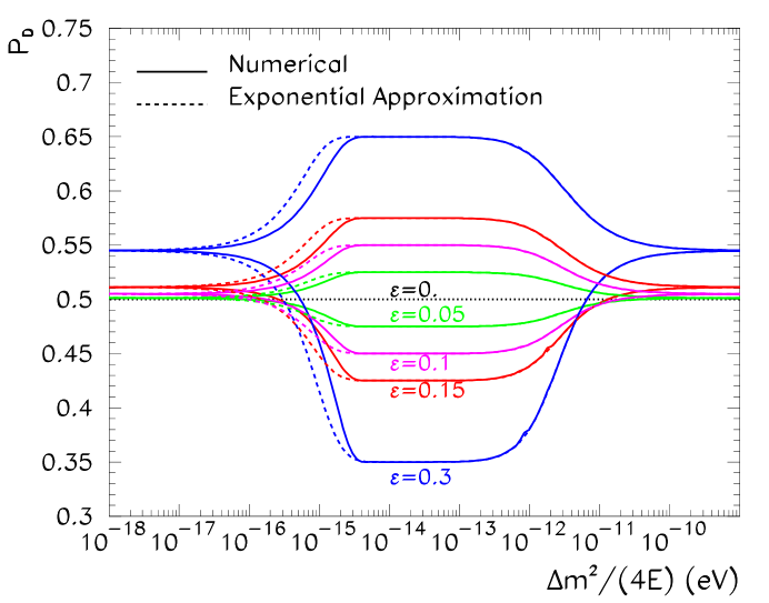
FIG. 1.: The dependence of the averaged $\nu_{e}$ survival probability inside the sun on $\Delta m^{2}/4E$ for different values of $\epsilon$ (numbers at the curves). The upper curves describe the corresponding negative values of $\epsilon$. Solid lines show results of numerical calculations. Dashed lines correspond to analytical formulae with exponential approximation for the solar density profile.

According to Eq. (28) and Fig. 1, in the MSW region (more precisely at the bottom of the suppression pit), the survival probability depends on $\epsilon$ linearly. For $\Delta m^{2}/E$ below and above the MSW region the probability converges to the vacuum oscillation probability. The deviation of the latter from the probability at maximal mixing depends on $\epsilon$ quadratically and the dependence on the sign of $\epsilon$ disappears. From this we infer that the sensitivity of $P_{D}$ and consequently of observables to $\epsilon$ is much higher in the MSW region.

Notice that there are two transition regions (between MSW and the vacuum oscillation regions) where the effects are mainly due to vacuum oscillations with small matter corrections. We call these regions ‘Quasi-Vacuum Oscillation regions’: we denote by QVO_L (QVO_S) the one with $\Delta m^{2}$ larger (smaller) than in the MSW region. In the QVO_L and QVO_S regions, the linear dependence of the probability and the observables transforms into quadratic dependence.

D Regeneration effects in the Earth

For a neutrino arriving at night time, Earth matter effects should be taken into account. To gain a qualitative understanding of the Earth effects, we make the crude approximation of uniform density, such that the mixing angle in the Earth is constant, $\theta_{E}$, along the neutrino trajectory. In this case, the neutrino propagation has an oscillatory character. We assume that the oscillations are averaged out, and therefore

$$P_{2e}(\mbox{\rm vacuum}) = \sin^{2}\theta,$$ (30)

$$P_{2e}(\mbox{\rm uniform\ density}) = {1\over 2}\left[\sin^{2}\theta+\sin^{2}(2\theta_{E}-\theta)\right].$$ (31)

It is convenient to introduce a regeneration factor which describes the Earth matter effect:

$$f_{\mbox{\rm reg}}\equiv P_{2e}({\mbox{\rm matter}})-P_{2e}({\mbox{\rm vacuum}})=\ {1\over 2}\sin 2\theta_{E}\sin(2\theta_{E}-2\theta).$$ (32)

Denoting by $\eta_{E}$ the parameter $\eta$ in the Earth:

$$\eta_{E}\equiv\eta(\rho_{E}Y_{eE}),$$ (33)

where $\eta$ is defined in Eq. (14), we find from Eq. (32):

$$f_{\mbox{\rm reg}}={\eta_{E}\sin^{2}2\theta\over 2(1-2\eta_{E}\cos 2\theta+\eta_{E}^{2})}.$$ (34)

Note that $f_{\mbox{\rm reg}}$ is always (for any value $\Delta m^{2}/E$ and $\epsilon$) positive, i.e. the matter effect of Earth always enhances the survival probability $P_{ee}$.

The parameter $f_{\mbox{\rm reg}}$ can be expanded around $\epsilon=0$:

$$f_{\mbox{\rm reg}}=\ {\eta_{E}\over 2(1+\eta_{E}^{2})}\left(1+{2\eta_{E}\over 1+\eta_{E}^{2}}\epsilon\right).$$ (35)

The regeneration factor has a maximum at $\eta_{E}\approx 1$ which corresponds to $\Delta m^{2}/E\sim(2-3)\times 10^{-13}$ eV. This determines the strong regeneration region in the $\Delta m^{2}/E$ scale. It is situated in the middle of the the solar MSW region. Strong regeneration effects are already excluded by the SuperKamiokande result on Day-Night asymmetry [32, 33]. Consequently, the strong regeneration region separates two (allowed) parts within the MSW region in which the regeneration effects are small:

1. HIGH $\Delta m^{2}$ region, where $\eta_{E}\gg 1$ and $f_{\mbox{\rm reg}}\sim 1/\eta_{E}$;

2. LOW $\Delta m^{2}$ region, where $\eta_{E}\ll 1$ and $f_{\mbox{\rm reg}}\sim\eta_{E}/2$.

We will quantify the borders of these regions in Sec. III. In both cases the regeneration effect is suppressed by a small parameter and it disappears when moving away from the strong regeneration region.

Let us stress that the SuperKamiokande limit on regeneration effects holds for the energy range $E=5-15$ MeV to which this experiment is sensitive. This corresponds to $\Delta m^{2}=(2-3)\times 10^{-6}$ eV². However, strong regeneration effects are not excluded for other energies, in particular, for low energy neutrinos. In this case $\eta_{E}$ can be of the order one and $f_{\mbox{\rm reg}}$ at its maximum.

To first order in $\epsilon$, we obtain from Eq. (35):

$$f_{\mbox{\rm reg}}=\left\{\begin{array}[]{ll}\frac{1}{2\eta_{E}}\left(1+\frac{2}{\eta_{E}}\epsilon\right)&({\rm HIGH})\\ \frac{\eta_{E}}{2}(1+2\eta_{E}\epsilon)&(\rm LOW)\end{array}\right..$$ (36)

In both the HIGH and LOW regions the dependence of the regeneration factor on $\epsilon$ is further suppressed by the small parameter min$\{2/\eta_{E},2\eta_{E}\}$.

The probability $P_{ee}$ at night time, $P_{N}$, can be written (for the region where the oscillating term in Eq. (9) is absent) as follows:

$$P_{N}\ =\ P_{1}+(1-2P_{1})\left(\sin^{2}\theta+f_{\mbox{\rm reg}}\right)=\frac{1}{2}+\frac{1}{2}(1-2P_{c})\cos 2\theta_{S}(\cos 2\theta-2f_{\mbox{\rm reg}}).$$ (37)

The average daily survival probability is given for $\eta_{S}\ll 1$ ($\cos 2\theta_{S}\approx-1$) by

$$\bar{P}\equiv{1\over 2}(P_{D}+P_{N})={1\over 2}[1+(1-2P_{1})(f_{\mbox{\rm reg}}-\cos 2\theta)].$$ (38)

The Day–Night asymmetry is given by

$$A_{\rm N-D}\equiv{P_{N}-P_{D}\over\bar{P}}={2f_{\mbox{\rm reg}}\over 1/(1-2P_{1})-\cos 2\theta+f_{\mbox{\rm reg}}}.$$ (39)

Let us now consider the dependence of $A_{N-D}$ and $\bar{P}$ on $\epsilon$ in the HIGH and in the LOW regions keeping the lowest order terms in $\epsilon$ and in min$\{\eta_{E},1/\eta_{E}\}$.

1. In the HIGH region, the adiabaticity condition is satisfied and we can safely put $P_{c}=0$. Consequently, $P_{1}=\cos^{2}\theta_{S}$. Then, Eq. (38) simplifies:

$$\bar{P}={1\over 2}[1-\cos 2\theta_{S}(f_{\mbox{\rm reg}}-\cos 2\theta)].$$ (40)

With near-maximal mixing, we obtain:

$$\bar{P}\ =\ {1\over 2}\left(1-\frac{\epsilon-1/2\eta_{E}}{\sqrt{1+\eta_{S}^{2}}}\right)+{\cal O}\left({1\over\eta_{E}\eta_{S}},{\epsilon\over\eta_{E}}\right).$$ (41)

For $\eta_{S}^{2}\ll 1$ (small $\Delta m^{2}$) we find:

$$\bar{P}\approx\frac{1}{2}\left(1-\epsilon+\frac{1}{2\eta_{E}}+\frac{\epsilon}{\eta_{E}^{2}}\right)~{},$$ (42)

where the last term is a small correction which comes from the regeneration factor. For the Day–Night asymmetry we obtain:

$$A_{\rm N-D}\ =\ {1\over\eta_{E}\sqrt{1+\eta_{S}^{2}}}\left[1+{(\sqrt{1+\eta_{S}^{2}}-\eta_{S}^{3})\epsilon\over 1+\eta_{S}^{2}}+{\cal O}\left({1\over\eta_{E}^{2}},{\epsilon\over\eta_{E}}\right)\right].$$ (43)

Notice that the $\epsilon$-dependent effect changes sign between large and small $\eta_{S}$. For $\eta_{S}^{2}\ll 1$ we get:

$$A_{\rm N-D}\simeq\frac{1}{\eta_{E}}(1+\epsilon)~{}.$$ (44)

The asymmetry increases linearly with $\epsilon$ for small enough $\eta_{S}^{2}$.

2. In the LOW region we can take $\eta_{S}=0$ and, consequently, $P_{1}=P_{c}$. Then, Eq. (38) simplifies:

$$\bar{P}=\frac{1}{2}\left[1+(1-2P_{c})(f_{\mbox{\rm reg}}-\epsilon)\right].$$ (45)

In LOW region we have $\gamma\gg 1$ (see Eq. (24)) and, therefore, $P_{c}\ll 1$ (see Eq. (23)). In any case, the $P_{c}$-dependent term in Eq. (45) is suppressed by a small factor and can be neglected. We get:

$$\bar{P}={1\over 2}\left(1-\epsilon+{\eta_{E}\over 2}\right).$$ (46)

For the Day-Night asymmetry we obtain taking $P_{c}\ll 1$:

$$A_{\rm N-D}\approx{2f_{\mbox{\rm reg}}\over 1+2P_{c}-\epsilon+f_{\mbox{\rm reg}}},$$ (47)

and in the limit $\eta_{E}\ll 1$:

$$A_{{\rm N-D}}=\eta_{E}\left(1-2e^{-\gamma/2}-{\eta_{E}\over 2}+\epsilon\right).$$ (48)

A few comments are in order. The Day–Night asymmetry is suppressed by $\eta_{E}$. The $\epsilon$-dependent effect is one of several small corrections to the leading result. For large parts of the LOW region it is the leading correction, but for large $\Delta m^{2}/E$, the subleading regeneration effect could be comparable while for small $\Delta m^{2}/E$, the non-adiabatic correction could give the main correction.

As we mentioned before, a strong regeneration effect with $\eta\sim 1$ and $f_{\mbox{\rm reg}}\sim 1$ is not excluded for low energy neutrinos. In particular in the LOW region strong regeneration can show up for the beryllium and pp-neutrino components of the spectrum. In this case, the approximation $\eta_{E}\ll 1$ does not work and one should use the complete expression for the regeneration factor and the asymmetry.

As seen from Eqs. (42), (46), (44) and (48), the dominant dependence on $\epsilon$ of both $\bar{P}$ and $A_{\rm N-D}$ arises from the dependence of the solar survival probability on $\epsilon$. The dependence which follows from the regeneration factor is further supressed by min$\{\eta_{E},1/\eta_{E}\}$. (For $A_{\rm N-D}$ the $\epsilon$ dependence follows from the dependence on $\bar{P}$ in the denominator.)

From Eqs. (44) and (48) we find that the Day-Night asymmetry strongly depends on $\Delta m^{2}$ due to the $\eta_{E}$ or $1/\eta_{E}$ factors. In the HIGH region $A_{\rm N-D}\propto\Delta m^{2}$ while in LOW region $A_{\rm N-D}\propto 1/\Delta m^{2}$. The dependence of the asymmetry on $\epsilon$ is much weaker: In both regions $A_{\rm N-D}\propto(1+\epsilon)$. Consequently, the measurements of $A_{\rm N-D}$ are very sensitive to $\Delta m^{2}$ while the sensitivity to $\epsilon$ is substantially lower.

Let us comment on the range of validity of the approximate treatment of the Earth effects [25]. In the HIGH region, for $E\sim$ MeV and $\Delta m^{2}\gg 10^{-6}\mbox{\rm eV}^{2}$, the oscillation length $l_{\nu}$ is much shorter than the size of the Earth and neutrinos undergo many oscillations inside the Earth. The constant electron number density approximation gives a good description of $A_{\rm N-D}$ which involves integration over the zenith angle. In the LOW region, for $\Delta m^{2}\ll 10^{-6}\mbox{\rm eV}^{2}$, the oscillation length is approximately equal to the refraction length $l_{0}$ and the latter is comparable to the size of the Earth (independently of $\Delta m^{2}$). The details of the $N_{e}$ profile do not play an important role, and the effect is determined by the average density along the neutrino trajectory.

Regeneration effect leads also to seasonal variations of signals [25, 26, 27]. These variations, however, are less sensitive to the oscillation parameters.

E Distortion of the energy spectrum

The distortion of the solar neutrino energy spectrum can be characterized by the distortion parameter defined as:

$$s_{\nu}\equiv\frac{E}{\bar{P}}\frac{d\bar{P}}{dE}.$$ (49)

Averaged over the appropriate energy interval this parameter is proportional to the shift of the first moment of the spectrum or to the slope parameter used in the literature.

To understand the distortion of the spectrum (energy dependence of the averaged probability), we remind the reader that $\eta\propto 1/E$ and use Eq. (40) for the HIGH and QVO_L regions and Eq. (45) for the LOW region.

1. The HIGH and QVO_L regions:

(i) For large $\Delta m^{2}$, the effect of the adiabatic edge of the suppression pit which is encoded in the $\eta_{S}$ dependence is important:

$$s_{\nu}\approx-\epsilon\frac{\eta_{S}^{2}}{(1+\eta_{S}^{2})^{3/2}}.$$ (50)

The distortion parameter is proportional to $\epsilon$. The slope (shift of the first moment) is positive (negative) for $\epsilon<0$ ($\epsilon>0$). The distortion decreases rapidly with $\eta_{S}$.

(ii) For small $\Delta m^{2}$, the earth regeneration which is related to the $\eta_{E}$ dependence is important:

$$s_{\nu}\approx\frac{1}{2\eta_{E}}\left(1+\epsilon-\frac{1}{2\eta_{E}}+\frac{4\epsilon}{\eta_{E}}\right).$$ (51)

The distortion decreases with increase of $\eta_{E}$ or $\Delta m^{2}$. The sensitivity to $\epsilon$ is much weaker than in the previous case and it follows mainly from the dependence on the average probability in the denominator.

2. The LOW region:

(i) For large $\Delta m^{2}$, the regeneration effect is important:

$$s_{\nu}\approx\frac{\eta_{E}}{2}(1+\epsilon).$$ (52)

The slope increases with $\eta_{E}$. The dependence on $\epsilon$ is weak.

(ii) For small $\Delta m^{2}$, the effect of the nonadiabatic edge of the solar suppression pit gives the dominant effect:

$$s_{\nu}=2\epsilon E\frac{dP_{c}}{dE}\approx\epsilon\gamma e^{-\gamma/2}.$$ (53)

The distortion is proportional to $\epsilon$. The slope is positive (negative) for $\epsilon>0$ ($\epsilon<0$). The effect is suppressed for relatively weak violation of the adiabaticity.

As we have mentioned previously, for non-averaged vacuum oscillations $s_{\nu}\propto(1-\epsilon^{2})$, that is, the dependence of distortion on $\epsilon^{2}$ is very weak.

F Summary

Let us summarize the results of our analytical studies. We have found simple analytical expressions for various observables (rates of events given by the survival probability, Day-Night asymmetry, distortion of the spectrum etc.) in terms of $\Delta m^{2}$ and the deviation from maximal mixing $\epsilon$. These approximate analytical expressions reproduce correctly the functional dependence of the observables on $\Delta m^{2}$ and $\epsilon$ and allow us to understand all the features of the exact numerical calculations.

The effects and the dependence of observables on $\epsilon$ change with $\Delta m^{2}$. Accordingly, we define several regions of $\Delta m^{2}$ which have different physical pictures. As $\Delta m^{2}$ decreases from its upper (CHOOZ) bound, we have the following regions (we quantify borders of these regions in the next section):

• quasi-vacuum oscillation region with large $\Delta m^{2}$ (QVO_L),

• MSW region with high $\Delta m^{2}$ (HIGH),

• MSW region with low $\Delta m^{2}$ (LOW),

• quasi-vacuum oscillation region with small $\Delta m^{2}$ (QVO_S),

• region of non-averaged vacuum oscillations (VO). The high $\Delta m^{2}$ part of the VO region will be called VAC_L.

As concerns the $\epsilon$ dependence of observables in these regions, we find two main conclusions:

1. Maximal mixing, $\epsilon=0$, is not a special point as far as the phenomenology is concerned (in contrast with theory). No divergencies or discontinuities appear in the dependence of observables on $\epsilon$. The dependence on $\epsilon$ is smooth and, in many cases, very weak. To mention a few examples: The day time survival probability is 1/2 at $\epsilon=0$. Earth regeneration effects, however, enhance the survival probability. In the MSW region the slope of the energy spectrum distortion is proportional to $\epsilon$ in certain regions of $\Delta m^{2}$, and consequently changes sign at $\epsilon=0$. The Day-Night asymmetry is proportional to $(1+\epsilon)$.

2. The character of the $\epsilon$-dependence of observables is different in the vacuum oscillations and MSW regions. In the regions of vacuum oscillation all the effects depend on $\epsilon$ quadratically. More precisely, the $\epsilon$-dependent factors are of two types:

$$1+\epsilon^{2} ({\rm averaged\ oscillations}),$$ (54)

$$1-\epsilon^{2} ({\rm non-averaged\ oscillations}).$$ (55)

The dependence is symmetric with respect to interchanging $\epsilon\leftrightarrow-\epsilon$. In the MSW regions (both HIGH and LOW), observables depend on $\epsilon$ linearly. Obviously the dependence is non-symmetric with respect to $\epsilon\leftrightarrow-\epsilon$. In the region of strong adiabatic conversion (bottom of the pit) we get for the survival probaility, the Day-Night asymmetry and the distortion parameter:

$$P_{D}\propto(1-\epsilon),~{}~{}~{}~{}~{}~{}A_{\rm N-D},~{}s_{\nu}\propto(1+\epsilon).$$ (56)

At the edges of the MSW region (edges of the suppression pit) we find

$$s_{\nu}\propto\epsilon.$$ (57)

The quasi-vacuum oscillation regions, QVO_L and QVO_S, are transition regions between the MSW and vacuum oscillation regions, where the linear dependence of observables transform into quadratic dependence.

Thus, for $\epsilon\ll 1$ the sensitivity of experiments to deviation from maximal mixing is much higher in the MSW regions. It will be difficult to measure $\epsilon$ near maximal mixing if $\Delta m^{2}$ turns out to be in the VO or QVO regions.

III Present Status of Maximal Mixing

In this section we describe the present status of maximal as well as near–maximal mixing. We use for this purpose the latest available results on solar neutrinos from Homestake [28], SAGE [29], GALLEX+GNO [30, 31], and the 1117 days of data sample of Super–Kamiokande [32, 33] experiments.

We calculate the acceptability of maximal and near–maximal mixing as a function of $\Delta m^{2}$ in the whole allowed range, that is, below the upper bound $\Delta m^{2}\leq 10^{-3}$ eV² from the reactor experiments [16, 34]. The goal of this study is to find excluded regions of the oscillation parameters $\Delta m^{2}-\epsilon$, as well as the regions of these parameters which are allowed and most plausible. We quantify our statements in terms of confidence level at which a given region is accepted (probability of realization) or excluded. We study the dependence of our conclusions on uncertainties in the solar neutrino fluxes (the SSM uncertainties) as well as on the procedure employed in the analysis. Some model- and the procedure-independent statements are formulated. The extent to which the results of this Section hold in a three generation framework with $|U_{e3}|\neq 0$ is discussed in Sec. VI.

A Global fit: allowed and forbidden regions

The results of a global fit to all existing experimental data on solar neutrinos are shown in Figs. 2$-$5. The analysis includes rates in Chlorine [28], Gallium [29, 30, 31], and Super–Kamiokande [32, 33] experiments, as well as the zenith angle dependence [32, 33] and the shape of the recoil electron spectrum [32, 33] in Super–Kamiokande.

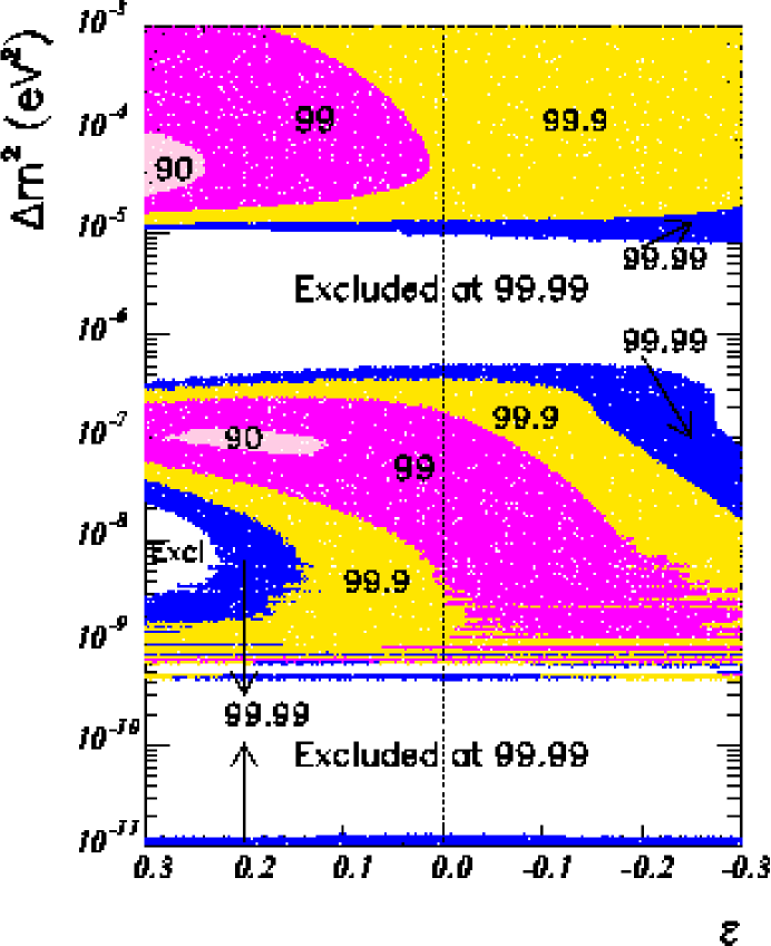
FIG. 2.: Contours of constant confidence level (iso-contours) in the $\Delta m^{2}-\epsilon$ plane. The shaded regions are accepted at the given or lower confidence level by the global fit of all available solar neutrino data. The white area is excluded at 99.99% confidence level.

In Fig. 2 we plot the contours of constant confidence level (iso–contours) in the $\Delta m^{2}-\epsilon$ plane. Points inside a given contour are accepted at a lower confidence level than on the contour itself. In the “global” analysis we combine the information on the Day–Night variation of the event rates and the recoil energy spectrum at Super–Kamiokande by using their independently measured spectra during the day and during the night. With this the total number of independent experimental inputs in the global analysis is 38 which includes 3 rates, and 35 data points for the Super–Kamiokande day and night recoil energy spectra ($2\times 18$ bins minus 1 overall normalization). We do not include in the analysis the new lower energy bin as its systematic uncertainty is still under study by the Super–Kamiokande Collaboration [33]. We use the solar neutrino fluxes from the Standard Solar Model (SSM) of Ref. [35] (BP98). The contours have been defined by the shift in $\chi^{2}$, $\Delta\chi^{2}$, with respect to the global minimum in the whole plane of the oscillation parameters. The minimum lies in the LMA solution region:

$$\chi^{2}=33.4\ \ \mbox{\rm for}\ 36\ \ \mbox{\rm d.o.f}.$$ (58)

which corresponds to a probability of 59%. For details on the statistical analysis we refer to Ref. [4].

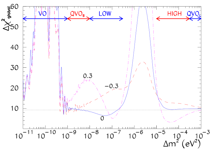
FIG. 3.: The dependence of $\Delta\chi^{2}$ from the global analysis (with the boron neutrino flux of the SSM) on $\Delta m^{2}$ for $\epsilon=-0.3$ (dashed line), $0$ (solid line) and $+0.3$ (dash-dotted line). Dotted horizontal line marks 99% CL. Below this line the corresponding oscillation parameters are accepted at a confidence level lower than 99%.

In Fig. 3 we show the dependence of $\Delta\chi^{2}$ on $\Delta m^{2}$ for three different values of $\epsilon$ ($-0.3,0,+0.3$). This figure corresponds to three $\Delta m^{2}$-profiles (cuts) of the confidence level from Fig. 2.

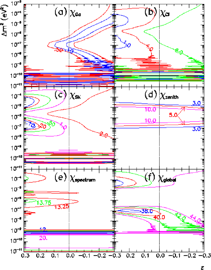
FIG. 4.: Contours of constant $\chi^{2}$ in the $\Delta m^{2}-\epsilon$ plane for individual experimental results. The various panels show the contributions of different results to the total $\chi^{2}$: (a) total rates in SAGE and GALLEX, (b) total rate in Homestake, and the Super–Kamiokande measurements of (c) the total rate, (d) zenith angle dependence, and (e) recoil electron energy spectrum. In (f) we show iso–contours of the total $\chi^{2}$.

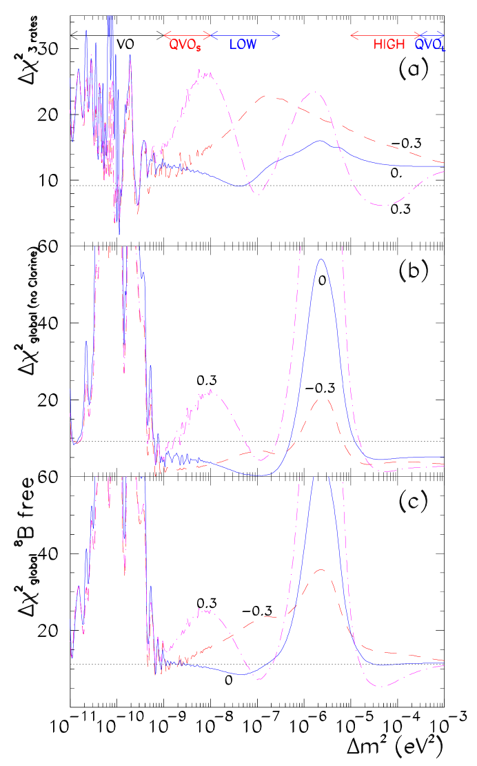
FIG. 5.: The dependence of $\Delta\chi^{2}$ on $\Delta m^{2}$ for $\epsilon=-0.3$ (dashed line), $0$ (solid line) and $0.3$ (dash-dotted line). Dotted horizontal lines mark 99% CL. Below this line the corresponding oscillation parameters are accepted at a confidence level lower than 99%. The three panels correspond to the following fits: (a) only total rates; (b) all the data except for the Homestake result; (c) all data with the boron neutrino flux treated as a free parameter.

What is the impact of individual experimental results on the global fit? Panels (a)$-$(f) of Fig. 4 show the contours of constant $\chi^{2}_{i}$ for each individual observable $i$. As mentioned above the total $\chi^{2}$ in panel (f) is obtained by combining the $\chi^{2}$ of the individual rates (including the correlation of their theoretical errors) with the corresponding $\chi^{2}$ for the Super–Kamiokande night and day recoil energy spectra.

Our calculations allow us to define regions of oscillation parameters that are excluded and other that are allowed. It follows from Fig. 2 that there are two main regions of $\Delta m^{2}$ which are excluded at a very high (more than $99.99\%$) confidence level:

1. The regeneration region: for maximal mixing we find

$$\Delta m^{2}=(0.6-8)\times 10^{-6}~{}~{}\mbox{\rm eV}^{2}~{}~{}~{}(\epsilon=0).$$ (59)

The excluded region increases with $\epsilon$ for positive values of $\epsilon$. In particular, for $\epsilon=0.3$, the excluded range becomes $\Delta m^{2}\sim(0.4-10)\times 10^{-6}\ \mbox{\rm eV}^{2}$. The excluded region also expands for negative values of $\epsilon$ at $\epsilon\mathrel{\hbox to0.0pt{\lower 4.0pt\hbox{\hskip 1.0pt$\sim$}\hss}\raise 1.0pt\hbox{$<$}}-0.25$.

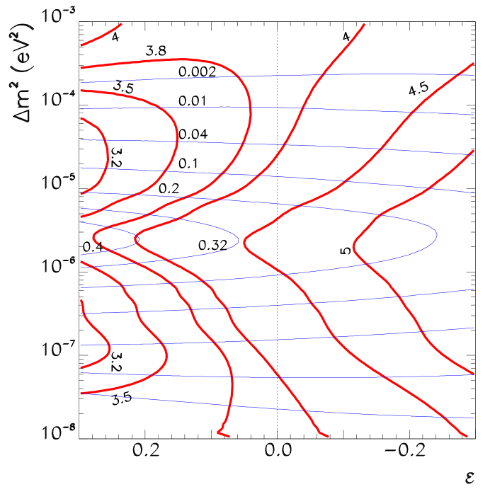
FIG. 6.: Contours of constant Day–Night asymmetry at Super–Kamiokande (thin lines) and of constant Ar–production rate (figures at the thick curves in SNU) in the $\Delta m^{2}-\epsilon$ plane.

In the regeneration region the solar neutrino observables are strongly modified by the $\nu_{e}$-regeneration in Earth. As we have discussed in Sec. II, the regeneration is always positive, thus leading to an increase in the $\nu_{e}$-flux. Correspondingly, the counting rates in all experiments increase. There are two main physical effects in the regeneration region that are inconsistent with observations and therefore lead to the exclusion:

(i) A large Day–Night asymmetry, $A_{\rm N-D}\mathrel{\hbox to0.0pt{\lower 4.0pt\hbox{\hskip 1.0pt$\sim$}\hss}\raise 1.0pt\hbox{$>$}}0.2$ (see Figs. 4(d) and 6), is in contradiction to the Super–Kamiokande result and plays a dominant role for positive $\epsilon$.

(ii) A large Ar–production rate, $Q_{Ar}>4$ SNU (see Figs. 4(b) and 6), is in contradiction to the Homestake result and leads to the increase of the excluded region for negative $\epsilon$.

2. The vacuum oscillation region:

$$\Delta m^{2}=(0.14-4)\times 10^{-10}~{}~{}\mbox{\rm eV}^{2}~{}~{}~{}(\epsilon=0).$$ (60)

The size of this region depends very weakly on $\epsilon$ in the interval $-0.3\mathrel{\hbox to0.0pt{\lower 4.0pt\hbox{\hskip 1.0pt$\sim$}\hss}\raise 1.0pt\hbox{$<$}}\epsilon\mathrel{\hbox to0.0pt{\lower 4.0pt\hbox{\hskip 1.0pt$\sim$}\hss}\raise 1.0pt\hbox{$<$}}+0.3$. The exclusion follows from the interplay between the total rates and the shape of the recoil electron energy spectrum. Notice that the rates only (see Fig. 5(a)) can be reproduced rather well in some parts of the region in Eq. (60). However, in these regions the distortion of the recoil electron spectrum is in contradiction with the Super–Kamiokande results (see Fig. 4(e)). More specifically, for $\Delta m^{2}\sim 10^{-10}$ eV², a negative slope (or shift of the first moment) in the “reduced” spectrum is expected. The reduced spectrum is defined as the ratio

$$R(E)\equiv N_{i}(E)/N_{i}(E)^{{\rm SSM}},$$ (61)

where $N_{i}(E)$ ($N_{i}(E)^{\rm SSM}$) is the number of events in a given electron energy, $E$, bin $i$ with (without) oscillations. In the same way we define any “reduced” observable as the ratio of its value with respect to the expected one in the SSM in the absence of oscillations.

3. There is another region forbidden at 99.99 % CL extending from $\Delta m^{2}=(0.3-2)\times 10^{-8}~{}~{}\mbox{\rm eV}^{2}$ for $\epsilon=0.3$ to $\Delta m^{2}=6\times 10^{-9}~{}~{}\mbox{\rm eV}^{2}$ and $\epsilon=0.22$. As seen in Fig. 3 this region is forbbiden with a lower CL. The exclusion follows mainly from the effect of the rates as seen in Fig. 5(a) being mainly driven by the bad fit to the Gallium rate (see Fig. 7(a)).

We distinguish five regions of the oscillation parameters where maximal mixing is allowed at a confidence level that is lower than 99.9%:

1) Quasi vacuum oscillation region with large $\Delta m^{2}$ (QVO_L):

$$\Delta m^{2}\sim\left(3\frac{E}{\rm 10\ MeV}-8\right)\times 10^{-4}\ \mbox{\rm eV}^{2},$$ (62)

where $E$ is the average detected energy for a given experiment. The upper bound comes from reactor experiments [16, 34]. Here the flavour conversion is mainly due to averaged vacuum oscillations with only small matter corrections inside the Sun and the Earth.

2) MSW region with high $\Delta m^{2}$ (HIGH):

$$\Delta m^{2}\sim\left(0.1-3\frac{E}{\rm 10\ MeV}\right)\times 10^{-4}\ \mbox{\rm eV}^{2}.$$ (63)

This region corresponds to the maximal and near–maximal mixing part of the LMA solution. It is restricted from below by strong Earth regeneration effects (large Day–Night asymmetry and large Ar–production rate). Maximal mixing is acceptable at confidence level larger than $99.1\%$. As follows from Fig. 3, the dependence of $\Delta\chi^{2}$ on $\Delta m^{2}$ is rather weak. The global fit becomes substantially better with increase of $\epsilon$ (shift to positive values): $\epsilon\mathrel{\hbox to0.0pt{\lower 4.0pt\hbox{\hskip 1.0pt$\sim$}\hss}\raise 1.0pt\hbox{$>$}}0.25$ is accepted at 90% CL. For $\epsilon=0.3$, the 90% CL allowed region expands to $\Delta m^{2}=(2-10)\times 10^{-5}$ eV². In contrast, the goodness of the fit decreases when we shift to negative values of $\epsilon$.

3) MSW region with low $\Delta m^{2}$ (LOW):

$$\Delta m^{2}\sim(0.1-3)\times 10^{-7}\ \mbox{\rm eV}^{2}.$$ (64)

Here maximal mixing is acceptable at $\sim 99\%$ CL in the interval

$$\Delta m^{2}\sim(0.1-2)\times 10^{-7}\ \mbox{\rm eV}^{2}\ (\mbox{\rm CL}\leq 99\%).$$ (65)

For positive $\epsilon$ the fit improves while for negative $\epsilon$ it worsens. In particular, $\epsilon=0.2$ is accepted at $\sim 90\%$ CL for $\Delta m^{2}\sim(0.8-1.5)\times 10^{-7}$ eV². The local minimum occurs at $\Delta m^{2}=1.0\times 10^{-7}\ \mbox{\rm eV}^{2}$ and $\epsilon=0.21$. With increase of $\epsilon$ the accepted region of $\Delta m^{2}$ shifts to larger values. At $\epsilon=0.3$ we obtain $\Delta m^{2}=(0.6-2)\times 10^{-7}\ \mbox{\rm eV}^{2}$. Conversely negative values of $\epsilon$ are disfavored.

4) Quasi vacuum oscillation region with small $\Delta m^{2}$ (QVO_S):

$$\Delta m^{2}\sim(0.1-1)\times 10^{-8}\ \mbox{\rm eV}^{2}.$$ (66)

In this region the flavour conversion is due to (mainly non-averaged) vacuum oscillations with small matter effects. Maximal mixing is acceptable at $\sim 99\%$ CL in the interval

$$\Delta m^{2}\sim(0.5-1)\times 10^{-8}\ \mbox{\rm eV}^{2}\ (\mbox{\rm CL}\sim 99\%).$$ (67)

The fit becomes worse with increase of $|\epsilon|$, but while for $\epsilon>0$ the QVO_S region is essentially excluded, for $\epsilon<0$ we still have a reasonably good fit.

5) Vacuum oscillation region with relatively large $\Delta m^{2}$ (VAC_L):

$$\Delta m^{2}\sim(0.4-1)\times 10^{-9}~{}~{}\mbox{\rm eV}^{2}.$$ (68)

Maximal mixing is accepted at a confidence level better than 99% only in a very small interval centered at:

$$\Delta m^{2}\sim 6.6\times 10^{-10}\ \mbox{\rm eV}^{2}~{}~{}~{}(\mbox{\rm CL}\leq 99\%).$$ (69)

In this interval, the goodness of the fit depends on $\epsilon$ very weakly.

Summarizing, maximal (or near–maximal) mixing is allowed at $99\%$ or slightly lower CL in several small intervals of $\Delta m^{2}$ in the QVO_L, HIGH, LOW, QVO_S and VAC_L solution domains. The values $\epsilon=0.05,~{}0.1,~{}0.2$ are allowed at 99, 95 and 90% CL, respectively. At $4\sigma$, practically the whole HIGH, LOW, QVO and VAC_L ranges are allowed.

Let us point out the role of individual experimental results in constraining maximal mixing (see Fig. 4). The rates in the Gallium and Super–Kamiokande experiments can be well accounted for at maximal (or near–maximal) mixing, although the Super–Kamiokande measurement slightly disfavors a negative $\epsilon$. The zenith angle distribution measured by Super–Kamiokande gives some preference to the HIGH region and excludes the strong regeneration region. In contrast, the Super–Kamiokande result on the recoil electron energy spectrum gives some preference to the VAC_L, HIGH and LOW regions and excludes the range $\Delta m^{2}=(0.3-4)\times 10^{-10}\ \mbox{\rm eV}^{2}$. Both the zenith angle distribution and the shape of spectrum have weak dependence on $\epsilon$. In contrast, total rates are sensitive to $\epsilon$, especially in the HIGH and LOW regions.

B Dependence of the results on features of the analysis

Let us study the dependence of the allowed and excluded regions in the $\Delta m^{2}-\epsilon$ plane on features of our analysis.

Total rates versus spectrum and zenith angle distribution: The total rates give the most stable, reliable, and statistically significant information. We have carried out a fit to the three rates only. In Fig. 5(a) we show the dependence of the shift of $\chi^{2}$ for this analysis with respect to the absolute minimum in the whole plane of oscillation parameters. The absolute minimum for the analysis of the three rates, $\chi^{2}=0.76$ (for one d.o.f) is achieved in the SMA region. Comparing Fig. 5(a) with Fig. 3, we learn that if we exclude the information from the recoil electron energy spectrum and the Day–Night variation of the event rates from our analysis, then the allowed and forbidden regions are substantially modified. In particular, we note in Fig. 5(a) the following three features:

(i) The goodness of the fit at maximal mixing from the analysis of the three rates only is worse in whole MSW region. At 99% CL only small interval in the LOW region is allowed. The fit improves however with increase of $\epsilon$. This means that it is the data on the spectrum and the zenith angle distribution which favor maximal mixing.

(ii) Allowed regions appear in the VAC solution range. We learn that the data on the spectrum and the zenith angle distribution exclude (otherwise) allowed VAC regions.

(iii) The regeneration region is still strongly disfavored by the high Ar–production rate.

The Homestake result: Consider the impact of the Ar–production rate on our results. In Fig. 4(b) we show the fit to only this rate. From the figure we see that the Homestake result strongly disfavors maximal mixing for all $\Delta m^{2}$ above $10^{-10}$ eV², that is, in all the globally allowed regions. In Fig. 5(b) we show the result of a global fit to the data without the Homestake result. Clearly, the acceptability of maximal mixing improves for all $\Delta m^{2}\mathrel{\hbox to0.0pt{\lower 4.0pt\hbox{\hskip 1.0pt$\sim$}\hss}\raise 1.0pt\hbox{$>$}}10^{-10}$ eV² with the best fit points being in the LOW region, $\Delta m^{2}=10^{-7}\ \mbox{\rm eV}^{2}$. For $\epsilon=0.3$ the best fit is in VAC_L region. We would like to emphasize the following points about a fit without the Homestake result:

(i) In the HIGH region, maximal mixing is accepted already at 1.7 $\sigma$ with very little dependence on $\epsilon$.

(ii) In the whole LOW region, maximal mixing gives a very good fit.

(iii) In the whole QVO_L region, maximal mixing gives a very good fit, but positive values of $\epsilon$ are still disfavored.

(iv) Regions of strong regeneration and VAC (small $\Delta m^{2}$) solutions are excluded by the Super–Kamiokande data on the spectrum and the Day–Night asymmetry.

Solar neutrino flux uncertainties: Of all the relevant solar neutrino fluxes, the boron neutrino flux suffers from the largest uncertainty, leading to systematic errors in the predicted detection rate that cannot be estimated reliably at present. One way to avoid this problem is to determine the boron neutrino flux experimentally, using the total rate measured in the Super–Kamiokande experiment. Similar results are obtained if the boron neutrino flux is treated as a free parameter in the analysis (in this case the Super–Kamiokande rate, being the most precise and sensitive to the boron neutrino flux, will fix this flux). In Fig. 5(c) we show the results of a global fit with the boron neutrino flux treated as a free parameter. We plot the dependence of $\Delta\chi^{2}$, the $\chi^{2}$ shift with respect to the absolute minimum, on $\Delta m^{2}$ for three different values of $\epsilon$. The shape of the curves is very similar to that in Fig. 3. Also the allowed and excluded regions at a given CL practically coincide with those in Fig. 3. (One should take into account that now we have one additional free parameter and therefore a 99% CL corresponds to $\Delta\chi^{2}=11.36$). The reason of this similarity lies on the fact that both the spectrum and the Day–Night variation are flux independent. Furthermore in both cases the boron neutrino flux is fixed by the Super–Kamiokande result.

A comparison of Fig. 3 and Fig. 5(c) shows that the results of our analysis are stable with respect to the way that the uncertainty in the boron neutrino flux is treated.

IV Maximal Mixing and Predictions for Individual Experiments

In this section we consider the predictions of (near–) maximal mixing for various observables. This will clarify the sensitivity of individual experiments to the neutrino oscillation parameters in the relevant range. The extent to which the results of this Section hold in a three generation framework with $|U_{e3}|\neq 0$ is discussed in Sec. VI.

A Total rates

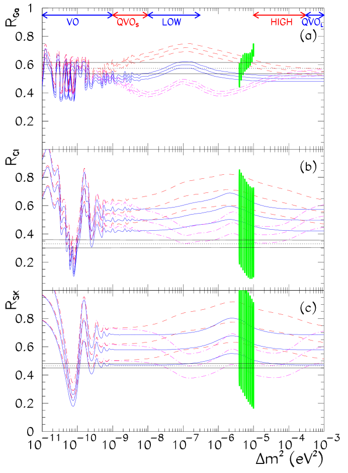
FIG. 7.: (a) The Germanium production rate, (b) the Argon production rate and (c) the rate of events at Super–Kamiokande, as functions of $\Delta m^{2}$ for 3 values of $\epsilon$: $+0.3$ (dash-dotted lines), $0$ (solid lines), $-0.3$ (dashed lines). The rates are normalized to the BP98 no oscillation expectation. Also shown are the experimental constraints and the SMA prediction. See the text for more details.

In Fig. 7 we plot the values of the expected event rates: Germanium production rate, Argon production rate, and the rate of events at Super–Kamiokande as functions of $\Delta m^{2}$ for 3 values of $\epsilon$: $+0.3,0,-0.3$. The rates are normalized to the no oscillation expectation, $R_{i}\equiv Q_{i}/Q_{i}^{{\rm SSM}}$. For each value of $\epsilon$ we plot three curves: the central curves give the expected rates using central values of the BP98 fluxes and the upper and lower lines represent the theoretical uncertainty (without the error for the interaction cross sections) from varying the nine parameters in the SSM within $\pm 1\sigma$. The horizontal lines give the experimental values within $\pm 1\sigma$ experimental errors. The vertical lines in the range $\Delta m^{2}=(3-10)\times 10^{-6}$ eV² give the expectation from the SMA 99% CL region (again, including the theoretical uncertainties in each point).

Let us first discuss the dependence of the rates on $\Delta m^{2}$. The rates are proportional to the survival probability. Therefore, the main features of Fig. 7 reflect the dependence of the survival probability on $\Delta m^{2}/E$ (see Fig. 1 and Eqs. (27), (28) and (29)). For maximal mixing the survival probability in the Sun as a function of $\Delta m^{2}/E$ is constant: $P_{D}=1/2$ (see Eq. (20)). The probability $P_{ee}$ is enhanced by the Earth regeneration effect for $\Delta m^{2}/E$ in the range $(10^{-15}-10^{-11})\ \mbox{\rm eV}$ (see Eq. (38)). For $\epsilon\neq 0$, the effects of the adiabatic edge situated at $\Delta m^{2}/E=(10^{-12}-10^{-10})$ eV (Eq. (42)), and of the non-adiabatic edge situated at $\Delta m^{2}/E=(10^{-16}-3\times 10^{-15})$ eV (Eq. (45)), become important. For $\Delta m^{2}/E\mathrel{\hbox to0.0pt{\lower 4.0pt\hbox{\hskip 1.0pt$\sim$}\hss}\raise 1.0pt\hbox{$<$}}10^{-16}$ eV, an oscillatory behaviour appears due to non-averaged vacuum oscillations between the Sun and the Earth (Eq. (29)). With certain modifications all these features can be seen in Fig. 7. The simplest dependence is for the Super–Kamiokande rate since only one (boron) neutrino flux contributes (Fig. 7(c)). The Ar–production rate has an additional fine structure due to contributions from additional fluxes, and in particular the beryllium neutrino flux. As can be seen from Fig. 7(b), an additional enhancement appears in the regeneration region at $\Delta m^{2}=3\times 10^{-7}\ \mbox{\rm eV}^{2}$ and the probability as a function of $\Delta m^{2}$ becomes asymmetric in the regeneration region. In the VAC and QVO_S regions the boron neutrino “wave” is modulated by the beryllium wave with a smaller amplitude. For the Ge–production rate, all the features of the curves are shifted (with respect to the Super–Kamiokande curves) to smaller values of $\Delta m^{2}$ by a factor $\sim 30$. This feature is due the fact that the main contribution to $Q_{Ge}$ comes from the $pp$-neutrino flux with an average detected energy of 0.3 MeV, about 30 times smaller than the average energy of the boron neutrino flux.

Let us consider now the $\epsilon$-dependence of the rates. We distinguish here between three different regions of $\Delta m^{2}$:

1) The QVO_L region with $\Delta m^{2}\mathrel{\hbox to0.0pt{\lower 4.0pt\hbox{\hskip 1.0pt$\sim$}\hss}\raise 1.0pt\hbox{$>$}}3\times 10^{-4}\ \mbox{\rm eV}^{2}$. Here we have essentially averaged vacuum oscillations, so that the survival probability is given by Eq. (27).

2) The QVO_S and VAC regions with $\Delta m^{2}\mathrel{\hbox to0.0pt{\lower 4.0pt\hbox{\hskip 1.0pt$\sim$}\hss}\raise 1.0pt\hbox{$<$}}10^{-8}\ \mbox{\rm eV}^{2}$. Here we have essentially non-averaged or partially averaged vacuum oscillations which take the form of Eq. (29). In principle matter effects strongly suppress the oscillations inside the Sun and the Earth. However, the modification of the observables is small, since the size of the Sun (and the Earth) is much smaller than the oscillation length in vacuum.

3) The matter conversion (MSW) region is between these two QVO regions. The oscillation effect is strongly suppressed. As explained in Sec. II, Earth matter effect is important but insensitive to $\epsilon$. The expression of $P$ in this region is given in Eqs. (42) and (45).

From Eqs. (27), (28), and (29) we can find straightforwardly the dependence of the observables on deviations from maximal mixing. For the VO, QVO_S and QVO_L regions, the following points are in order:

1. The observables depend very weakly on $\epsilon$. Corrections to maximal mixing are of ${\cal O}(\epsilon^{2})$.

2. The dependence is symmetric under the exchange $\epsilon\leftrightarrow-\epsilon$. Minimum of the survival probability, and consequently, minima of rates, are at $\epsilon=0$, that is, at maximal mixing.

For the MSW regions, the following points are in order:

1. The survival probability and the rates depend linearly on $\epsilon$. Corrections to the maximal mixing case are consequently larger.

2. The survival probability and the rates decrease with increase of $\epsilon$.

There are two transition regions between VO and pure matter conversion. In these regions, the symmetric dependence of the observables transforms into a linear dependence and the sensitivity to deviation from maximal mixing increases. The ambiguity $\epsilon\leftrightarrow-\epsilon$ disappears.

Thus, in the region of pure matter conversion (inside the Sun) the sensitivity of measurements of rates to a deviation from maximal mixing is maximal. It is in this region that the possibility of maximal mixing can be tested with the highest accuracy. The corresponding $\Delta m^{2}$ range depends on the neutrino energy. For the highest energies of the solar neutrinos ($E\sim 10$ MeV) we get the range of maximal sensitivity: $\Delta m^{2}=10^{-7}-10^{-4}~{}\mbox{\rm eV}^{2}$, while for the lowest energies ($E\sim 0.3$ MeV) the range is $\Delta m^{2}=3\times 10^{-9}-3\times 10^{-6}~{}\mbox{\rm eV}^{2}$. Studying effects by the experiments with different energy thresholds we can get high sensitivity to deviations from maximal mixing in whole range of $\Delta m^{2}$ excluding VO.

In the next two subsections we consider the dependence of specific rates on the oscillation parameters and evaluate the sensitivity of their present measurements to deviations from maximal mixing.

B Ar–production rate.

Let us now study the implications of the results presented in Fig. 7(b) for the Ar–production rate and in Fig. 7(c) for the Super–Kamiokande rate in the various $\Delta m^{2}$ regions. As can be seen in Fig. 7(b), the Ar–production rate for maximal mixing in all favorable regions (HIGH, LOW, VAC_L) lies in the range $R_{Cl}=0.50\pm 0.08$ ($Q_{Ar}=3.9\pm 0.6$ SNU), which is $2\sigma$ above the Homestake result. The predictions for $\epsilon=+0.3$ ($-0.3$) are below (above) the values for maximal mixing by just about $1\sigma$. As mentioned above, the highest sensitivity of $Q_{Ar}$ to $\epsilon$ is achieved already in the HIGH region, where $Q_{Ar}$ depends on $\epsilon$ linearly. For the Super–Kamiokande rate, we get that for maximal mixing in all favorable regions $R_{SK}=0.58\pm 0.12$ which is $1\sigma$ above the Super–Kamiokande result. Moreover comparing Figs. 7(b) and  7(c) we see that the Ar–production rate and the Super–Kamiokande rate are strongly correlated as they are both dominated by the contribution from boron flux neutrinos.

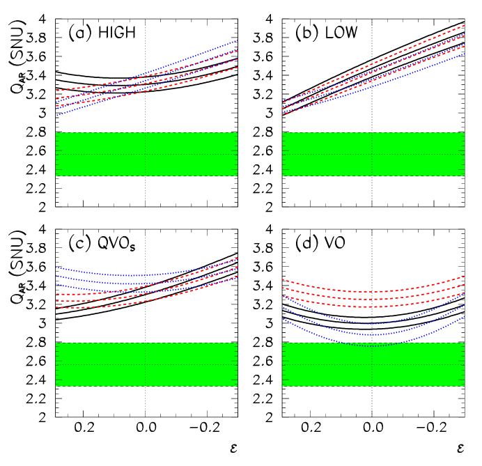
FIG. 8.: The dependence of the Ar–production rate on $\epsilon$ for various values of $\Delta m^{2}$ within the (a) HIGH, (b) LOW, (c) QVO_S and (d) VO regions. Full, dashed and dotted lines correspond to: (a) $\Delta m^{2}=4,\ 0.8,$ and $0.2\times 10^{-5}$ eV², (b) $\Delta m^{2}=1,\ 0.7,$ and $0.3\times 10^{-7}$ eV², (c) $\Delta m^{2}=10,\ 5,$ and $1\times 10^{-9}$ eV², (d) $\Delta m^{2}=5,\ 0.3,$ and $1\times 10^{-10}$ eV², respectively. For each mass the three curves correspond to the predicted central value plus and minus 1$\sigma$ theoretical uncertainties. The boron neutrino flux is normalized to the measured rate at Super–Kamiokande. The horizontal band corresponds to the Homestake experimental result and its 1$\sigma$ error.

Next, in order to reduce the SSM uncertainty we normalize the boron neutrino flux to the Super–Kamiokande rate. More precisely, for each pair of the of oscillation parameters ($\Delta m^{2},\epsilon$) we find the boron neutrino flux which reproduces the Super–Kamiokande event rate. All other fluxes and their uncertainties are taken according to the BP98. Using this procedure we calculate $Q_{Ar}$ (and in the next subsection also $Q_{Ge}$). The results of this calculation are shown in Fig. 8.

From Fig. 8 we see that after boron flux normalization procedure the dependence of $Q_{Ar}$ on $\epsilon$ is relatively weak since the ratio between the boron neutrino flux contribution to $Q_{Ar}$ and the contribution from charged current interactions to the Super–Kamiokande rate is independent of the survival probability and therefore of $\epsilon$. The $\epsilon$ dependence of $Q_{Ar}$ comes directly from the suppression of the beryllium and other (CNO and pep) neutrino fluxes, and indirectly from the contribution of neutral current interactions to the Super–Kamiokande rate. Expressing the boron neutrino flux $f_{B}$ via the SK rate:

$$f_{B}\sim\frac{R_{SK}}{P(1-r)+r},$$ (70)

we obtain:

$$Q_{Ar}\sim\frac{Q_{Ar}^{B}R_{SK}}{(1-r+r/P)}+Q_{Ar}^{\not B}P^{\prime}.$$ (71)

Here $r$ is the ratio of the $\nu_{\mu}-e$ and $\nu_{e}-e$ cross-sections, $Q_{Ar}^{B}$ and $Q_{Ar}^{\not B}$ are the SSM contributions to the Ar–production rate from the boron neutrino flux and from all other low energy fluxes, respectively, and $P$ and $P^{\prime}$ are the effective survival probabilities for the boron neutrino and low energy neutrino fluxes, respectively. The bands in Fig. 8 reflect $1\sigma$ errors due to the uncertainties in all, but the boron, neutrino fluxes.

As expected, in the QVO regions, QVO_L and QVO_S, the $\epsilon$-dependence is symmetric around $\epsilon=0$, $Q_{Ar}=Q_{Ar}(\epsilon^{2})$, while in the pure matter conversion regions, HIGH and LOW, $Q_{Ar}$ depends on $\epsilon$ linearly. In the linear regime, the change in the Ar–production rate is $\Delta Q_{Ar}\sim(0.7-0.8)$ SNU for $-0.3\mathrel{\hbox to0.0pt{\lower 4.0pt\hbox{\hskip 1.0pt$\sim$}\hss}\raise 1.0pt\hbox{$<$}}\epsilon\mathrel{\hbox to0.0pt{\lower 4.0pt\hbox{\hskip 1.0pt$\sim$}\hss}\raise 1.0pt\hbox{$<$}}+0.3$. This is about $3\sigma$ for the present experimental error. In the quadratic regime the change is substantially smaller: $\Delta Q_{Ar}\sim(0.1-0.2)$ SNU. Clearly, the present sensitivity is not enough to draw definite conclusions. Moreover, even after normalization of the boron neutrino flux to the Super–Kamiokande rate, the predicted rate is higher than the Homestake result for all globally allowed values of $\Delta m^{2}$. The only statement that one can make is that the Homestake result favors a significant deviation from maximal mixing in the MSW region. Therefore checks of the Homestake result and improved accuracy in measurements of $Q_{Ar}$ by a factor of two or higher would have important implications for maximal and near–maximal mixing.

C Ge–production rate

Let us now study the implications of the results presented in Fig. 7(a) where we show the Ge–production rate as a function of $\Delta m^{2}$ for different values of the $\epsilon$ parameter and in and Fig. 9 where we plot $Q_{Ge}$ as a function of $\epsilon$ in the various $\Delta m^{2}$ regions. While the results plotted in Fig. 7(a) are obtained within the SSM, the predicted rates shown in Fig. 9 have been obtained after normalization of the boron neutrino flux to the Super–Kamiokande measured rate as described previously for Fig. 8. In this case, unlike in the case of Ar–production rate, the results are very slightly modified by the ${}^{8}B$ flux normalization since the Ge–production rate is dominated by the contribution from the $pp$ neutrino flux and the corresponding theoretical uncertainties are smaller.

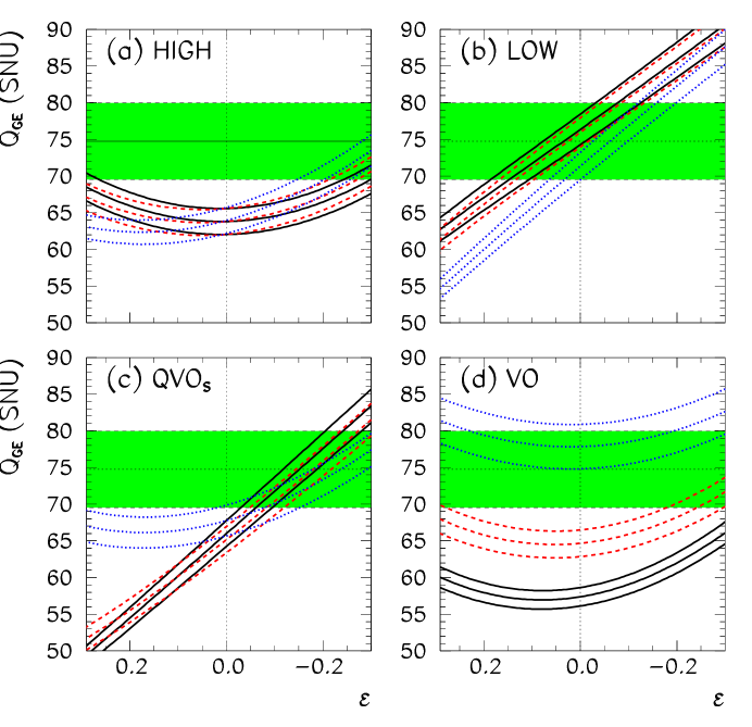
FIG. 9.: The dependence of the Ge–production rate on $\epsilon$ for various values of $\Delta m^{2}$ within the (a) HIGH, (b) LOW, (c) QVO_S and (d) VO regions. Full, dashed and dotted lines correspond to: (a) $\Delta m^{2}=4,\ 0.8,$ and $0.2\times 10^{-5}$ eV², (b) $\Delta m^{2}=1,\ 0.7,$ and $0.3\times 10^{-7}$ eV², (c) $\Delta m^{2}=10,\ 5,$ and $1\times 10^{-9}$ eV², (d) $\Delta m^{2}=5,.3,$ and $1\times 10^{-10}$ eV², respectively. For each mass the three curves correspond to the predicted central value plus and minus 1$\sigma$ theoretical uncertainties. The boron neutrino flux is normalized to the measured rate at Super–Kamiokande. The horizontal band corresponds to the averaged Gallium result and its 1$\sigma$ error.

In the QVO_L region, the rate is determined by averaged vacuum oscillations and therefore the expected rate is symmetric around maximal mixing. According to Eq. (29), $P(\epsilon=\pm 0.3)=0.545$ which corresponds to $Q_{Ge}=70.3\pm 3.5$ SNU (with $1\sigma$ theoretical error). For exactly maximal mixing we have $P(\epsilon=0)=0.5$ and the rate is minimal, $Q_{Ge}=64.5\pm 3.5$ SNU. As seen in Fig. 7(a) the bands for the different $\epsilon$-values almost overlap and all the predictions are in agreement with the present experimental result. In other words, with present experimental error bars it is impossible to measure deviations from maximal mixing.

In the part of the HIGH region with small $\Delta m^{2}$ the effects for $pp$ neutrinos occur in the transition between linear and quadratic $\epsilon$ regimes. Consequently, the sensitivity of $Q_{Ge}$ to $\epsilon$ is still below the present experimental accuracy. We find from Fig. 7(a): $Q_{Ge}(\epsilon=0)\approx Q_{Ge}(\epsilon=+0.3)\approx 60-68$ SNU, while $Q_{Ge}(\epsilon=-0.3)\approx 70\pm 4$ SNU, approximately $1\sigma$ (experimental) higher. From Fig. 9(a) we see that after the ${}^{8}B$ normalization the variation of the $Q_{Ge}$ in $\epsilon$ range $(-0.3,+0.3)$ is $\Delta Q_{Ge}\sim(10-12)$ SNU, which is about $2\sigma$ (present experimental error).

In the LOW region the sensitivity to $\epsilon$ is maximal: the $pp$ neutrinos undergo pure matter conversion and the rate depends on $\epsilon$ linearly. We get, for $\Delta m^{2}=10^{-7}\ \mbox{\rm eV}^{2}$: $Q_{Ge}(\epsilon=-0.3)=93\pm 4$ SNU, $Q_{Ge}(\epsilon=0)=77.5\pm 3.5$ SNU and $Q_{Ge}(\epsilon=0.3)=61\pm 3$ SNU. The difference between the predicted values of $Q_{Ge}(\epsilon=-0.3)$ and $Q_{Ge}(\epsilon=+0.3)$ is more than $2\sigma$ (experimental). From Fig. 9(b) we see that after the ${}^{8}B$ normalization the variation of the $Q_{Ge}$ in $\epsilon$ range $(-0.3,+0.3)$ is $\Delta Q_{Ge}\sim(33-35)$ SNU, which is more than $5\sigma$ (present experimental error). In this case one gets certain restrictions on $\epsilon$, although the confidence level is low. For example, for $\Delta m^{2}=10^{-7}\ \mbox{\rm eV}^{2}$, the combined SAGE and GALLEX+GNO result gives the $1\sigma$ range $-0.12\leq\epsilon\leq+0.2$. Therefore, further decrease of the experimental error bars by a factor of two, from the present 5 SNU to 3 - 4 SNU, could have important implications for the mixing provided that $\Delta m^{2}$ will be fixed by some other independent measurement. Notice that in the LOW region one expects maximal regeneration effect for the $pp$-neutrinos which can be detected as, e.g., seasonal variation of the Ge–production rate [27].

The situation is similar in the QVO_S region down to $\Delta m^{2}=5\times 10^{-9}\ \mbox{\rm eV}^{2}$: the Ge–production rate depends on $\epsilon$ linearly and $\Delta Q_{Ge}\sim 30$ SNU (see Fig. 9(c)).

In the VO region, deviations from the maximal mixing result are determined by $\epsilon^{2}$ and the variations (for a given $\Delta m^{2}$) are small as shown in Fig. 9(d): $\Delta Q_{Ge}\sim 5-7$ SNU. Thus the sensitivity of present data is still low and practically the whole interval $\epsilon\in(-0.3,+0.3)$ is allowed at $(2-3)\sigma$ level.

In consequence serious implications for maximal mixing require further decrease of the experimental error bars down to 3-4 SNU.

D The Day–Night asymmetry in electron scattering events

In Fig. 6 we show contours of constant Day–Night asymmetry of the $\nu-e$ scattering events in the $\Delta m^{2}-\epsilon$ plane. The Super–Kamiokande 1117 days result

$$A_{{\rm N-D}}=2\frac{N-D}{N+D}\sim 0.034\pm 0.026\;$$ (72)

excludes at the $3\sigma$ level the region $A_{{\rm N-D}}\mathrel{\hbox to0.0pt{\lower 4.0pt\hbox{\hskip 1.0pt$\sim$}\hss}\raise 1.0pt\hbox{$>$}}0.11$ which corresponds, at maximal mixing, to

$$4\times 10^{-7}\mathrel{\hbox to0.0pt{\lower 4.0pt\hbox{\hskip 1.0pt$\sim$}\hss}\raise 1.0pt\hbox{$<$}}\Delta m^{2}\mathrel{\hbox to0.0pt{\lower 4.0pt\hbox{\hskip 1.0pt$\sim$}\hss}\raise 1.0pt\hbox{$<$}}1.3\times 10^{-5}\ \mbox{\rm eV}^{2}.$$ (73)

The exclusion interval increases slightly with $\epsilon$. The preferable regions of $\Delta m^{2}$ for $\epsilon=0$ are

$$\Delta m^{2}=(2.5-10)\times 10^{-5}\ \mbox{\rm eV}^{2},~{}~{}~{}~{}\Delta m^{2}=(0.6-2.2)\times 10^{-7}\ \mbox{\rm eV}^{2}.$$ (74)

We emphasize that these results are SSM independent and have no ambiguities related to the analysis of the data.

E Zenith angle distribution of electron scattering events

In Fig. 10 we show the zenith angle distribution of events in Super–Kamiokande for maximal and near–maximal mixing and for various values of $\Delta m^{2}$ from the allowed regions. Significant enhancement of the night rate is expected in the HIGH and LOW regions.

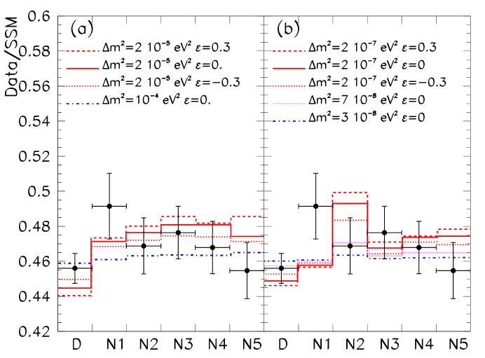
FIG. 10.: The zenith angle distribution of events in Super–Kamiokande and the predictions with (near–)maximal mixing for various values of $\Delta m^{2}$ within the (a) HIGH and (b) LOW regions.

In the HIGH region the distribution of events during the night is rather flat and the dependence on $\epsilon$ is weak, so it will be difficult to use the shape to measure $\epsilon$. The dependence on $\Delta m^{2}$ is also weak. Maximal signal is expected in the N3 or/and N5 (core) bins.

In the LOW region the oscillations occur in the matter dominated regime (see Sec. II) when the oscillation length practically coincides with the refraction length, $l_{m}\approx l_{0}$. For those trajectories crossing the mantle only (N1-N4), the latter can be approximately determined by the average density along the trajectory. Maximal effect (which corresponds to the oscillation phase $=\pi$) is realized for the trajectories with $\cos\theta_{Z}=0.3$, i.e. in the N2 bin (see Fig. 10(b)). The phase $2\pi$ is collected at $\cos\theta_{Z}\sim 0.5$ which corresponds to a minimum of the signal. Notice also that the zenith angle distribution depends on $\epsilon$ very weakly. For a given trajectory the amplitude of the oscillation is determined by the mixing angle in the Earth matter

$$\sin^{2}2\theta_{E}\sim\frac{1}{\eta_{E}^{-2}+1-2\epsilon\eta_{E}^{-1}}$$ (75)

where $\eta_{E}$ the parameter $\eta$ in the Earth defined in Eq. (33). Thus $\sin^{2}2\theta_{E}$ is an increasing function of $\epsilon$ (see also Eq. (18)). As a consequence the number of events in maxima increases with $\epsilon$ as seen in Fig. 10(b). Present data do not show any enhancement in the N2 bin.

We conclude that precise measurements of the zenith angle distribution would allow the determination of $\Delta m^{2}$ and probably resolve the HIGH/LOW ambiguity but are unlikely to play a significant role in the determination of $\epsilon$.

F The recoil electron energy spectrum

In Fig. 11 we show the expected recoil electron spectrum for maximal mixing with various values of $\Delta m^{2}$ in the regions allowed by the global fit. In the HIGH and LOW regions the “reduced” spectra, $R(E)$, are flat. Strong distortion is expected in the VAC_L region. Thus further improvement on the measurement of the recoil electron spectrum can discriminate between the MSW and VAC_L regions.

For large enough $\Delta m^{2}$ and $\epsilon\neq 0$ a distortion in the spectrum appears due to the effect of the adiabatic edge (Fig. 12(a)). This feature can be traced from the dependence of the survival probability on $\Delta m^{2}/E$ (see Fig. 1). For a positive $\epsilon$ conversion inside the sun leads to negative slope of the reduced spectrum: $R(E)$ is larger at low energies. For negative $\epsilon$, $R(E)$ increases with $E$ and the slope is positive. In the small $\Delta m^{2}$ part of the LOW region the distortion of the spectrum is induced by the effect of the non-adiabatic edge (Fig. 1, $\Delta m^{2}/4E=(0.3-3)\times 10^{-15}$ eV. Here the situation is opposite to that for the HIGH region. The slope is positive for positive $\epsilon$ and negative for negative $\epsilon$ as illustrated in Fig. 12(b).

As follows from Figs. 11 and 12, the measurement of the electron energy spectrum provides information mainly on the value of $\Delta m^{2}$ but it will be difficult to determine $\epsilon$ by measuring the slope (first moment of the spectrum) in the interval $-0.3\leq\epsilon\leq 0.3$ at Super–Kamiokande. At present Super–Kamiokande has presented the measured value $\langle T\rangle=8.14\pm 0.02$ MeV. The precision of this measurement is to be compared with the maximum theoretically expected variation $\Delta\langle T\rangle=|\langle T\rangle(\epsilon=0.3)-\langle T\rangle(\epsilon=-0.3)|<0.025$ MeV which occurs for the two values of $\Delta m^{2}$ shown in Fig. 12. Thus with the existing experimental precision, in the MSW region, the full range of $\epsilon$ is allowed at $\sim$ 1$\sigma$.

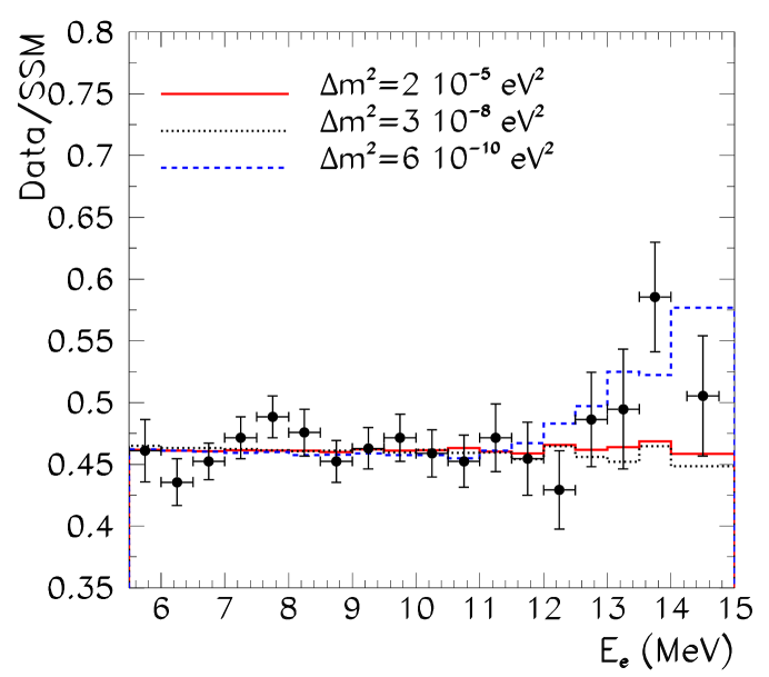
FIG. 11.: The “reduced” spectrum for Super–Kamiokande for $\epsilon=0$ and various values of $\Delta m^{2}$.

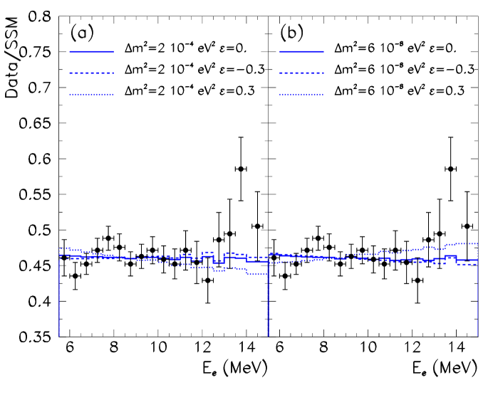
FIG. 12.: The “reduced” spectrum for Super–Kamiokande for (a) $\Delta m^{2}=2\times 10^{-4}$ eV² and (b) $\Delta m^{2}=6\times 10^{-8}$ eV² with $\epsilon=-0.3,0,0.3$.

V Tests of Maximal Mixing in Future Experiments

In this section we consider the prospects of testing (near–)maximal mixing of the electron neutrinos in future experiments. We study various possibilities to measure the deviation $\epsilon$ and we estimate the accuracy at which maximal mixing can be established or excluded. The extent to which the results of this Section hold in a three generation framework with $|U_{e3}|\neq 0$ is discussed in Sec. VI.

A General requirements

There are two requirements for a precise determination of the mixing:

1. Uncertainties in the original neutrino fluxes should not play a role. For this purpose we will consider SSM independent observables, or at least observables which do not depend on the uncertainties in the boron neutrino flux.

2. At least two independent observables should be measured. As we have seen in Sec. III, the survival probability $P_{ee}$ and consequently all observables depend on both $\epsilon$ and $\Delta m^{2}$. Even in the case of maximal mixing when the solar survival probability is constant, $P_{D}=1/2$, a dependence of $P_{ee}$ on $\Delta m^{2}$ appears due to the Earth regeneration effect.

Thus, to determine the mixing, one should find two independent observables which (i) are free of flux uncertainties, (ii) can be measured with high accuracy, and (iii) depend on different combinations of $\epsilon$ and $\Delta m^{2}$. In what follows we will identify such observables and study the accuracy at which mixing can be measured.

B GNO and Super–Kamiokande

The main objective of the GNO experiment [31] is to reach an accuracy $\sim 3$ SNU in the measurement of the Ge–production rate, $Q_{Ge}$. Also seasonal variations of $Q_{Ge}$ will be studied. Super–Kamiokande will continue to collect data for at least 10 years. With an energy threshold as low as 5 MeV the accuracy in measuring the Day–Night asymmetry will improve to $\sim 0.010-0.015$.

Notice that, in the MSW region, $A_{\rm N-D}$ is mostly sensitive to $\Delta m^{2}$, whereas $Q_{Ge}$ has strong dependence on $\epsilon$. Therefore the pair of observables ($A_{{\rm N-D}},Q_{Ge}$) is, in principle, very useful for measurements of the oscillation parameters in the matter conversion region.

In Fig. 13 we show simultaneously contours of constant $A_{\rm N-D}$ at Super–Kamiokande site and $Q_{Ge}$ in the $\Delta m^{2}-\epsilon$ plane. The iso–contours for $Q_{Ge}$ have been obtained for central values of the solar fluxes according to BP98. The theoretical (1$\sigma$) uncertainty is about $\pm 2$ SNU.

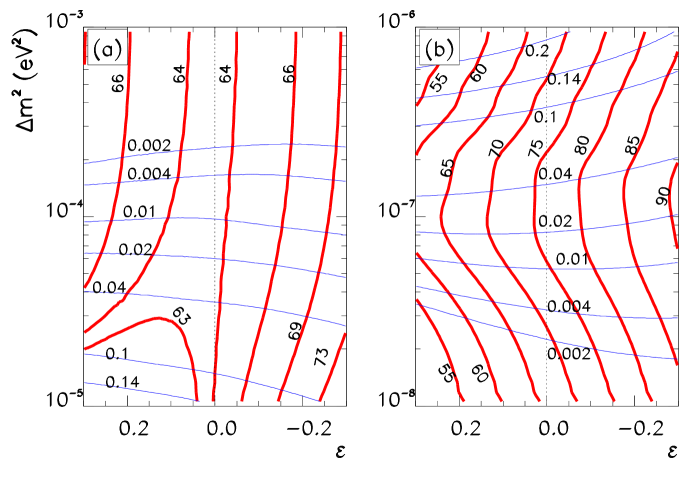
FIG. 13.: Iso–contours of $A_{{\rm N-D}}$ at Super-Kamiokande (thin lines) and of $Q_{Ge}$ (thick curves with numbers in SNU) in the $\Delta m^{2}-\epsilon$ plane for the HIGH (a) and LOW (b) regions.

The iso-contours of $Q_{Ge}$ and $A_{{\rm N-D}}$ are nearly perpendicular to each other, which reflects the fact that these observables depend on different combinations of the oscillation parameters. However, the accuracy of the present experimental results is not enough to put statistically significant bounds on the mixing. The present experimental $1\sigma$ intervals are $Q_{Ge}\sim 69-80$ SNU and $A_{\rm N-D}\sim 0.01-0.06$. The resulting constraints on the mixing parameters can be read from Fig. 13: in the HIGH region, $-0.2\mathrel{\hbox to0.0pt{\lower 4.0pt\hbox{\hskip 1.0pt$\sim$}\hss}\raise 1.0pt\hbox{$>$}}\epsilon$ and $\Delta m^{2}\sim(1.5-8)\times 10^{-5}\ \mbox{\rm eV}^{2}$, and in the LOW region $-0.10\mathrel{\hbox to0.0pt{\lower 4.0pt\hbox{\hskip 1.0pt$\sim$}\hss}\raise 1.0pt\hbox{$<$}}\epsilon\mathrel{\hbox to0.0pt{\lower 4.0pt\hbox{\hskip 1.0pt$\sim$}\hss}\raise 1.0pt\hbox{$<$}}+0.15$ and $\Delta m^{2}\sim(0.5-2)\times 10^{-7}\ \mbox{\rm eV}^{2}$. Inclusion of the theoretical uncertainties will expand these regions, especially in the HIGH case where the sensitivity of $Q_{Ge}$ to $\epsilon$ is rather low.

Notice that the present Gallium data somewhat disfavor maximal mixing in the HIGH region. We estimate that the $1\sigma$ accuracy of the determination of $\epsilon$ is

$$\Delta\epsilon\approx 0.15-0.20,~{}~{}~{}~{}(1\sigma).$$ (76)

Within $2\sigma$ experimental errors the allowed regions cover most of HIGH parameter space of Fig. 13(a), and practically the entire LOW parameter space of Fig. 13(b). All values of $\epsilon\in(-0.3,+0.3)$ become allowed at the $2\sigma$ level.

With more data from GNO and higher statistics Super–Kamiokande measurements of the asymmetry one can reach better sensitivity.

C SNO

The SNO experiment [36] will study various observables in three types of processes:

1. Charged current neutrino-deuteron scattering: the total rate above a certain threshold (we denote the reduced rate of events by [CC]), the energy distribution of events (electron energy spectrum), and the time variation of events which can be characterized by the Day-Night asymmetry $A_{\rm N-D}^{\rm CC}$, the zenith angle distribution, and the seasonal asymmetry.

2. Neutrino-electron scattering: the total rate [ES], electron energy spectrum, and time variations.

3. Neutral current neutrino-deuteron scattering: the total rate [NC], and time variations.

Since the SNO observables depend on the boron neutrino flux only (we neglect the effect of the hep-neutrino flux), the ratios of rates are flux independent. Also relative time variations and energy spectrum distortion are flux independent. In what follows all the results will be presented for an energy threshold of 5 MeV.

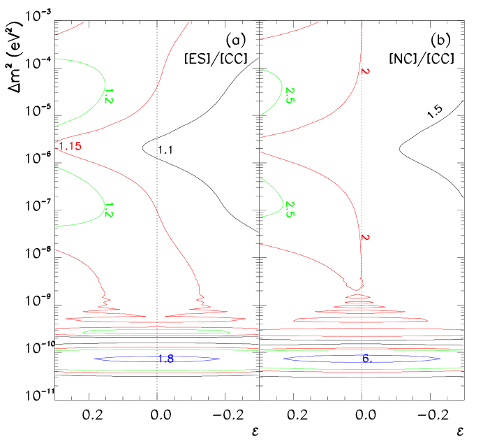
FIG. 14.: Iso-contours of the double ratios of rates in the $\Delta m^{2}-\epsilon$ plane: (a) [ES]/[CC]; (b) [NC]/[CC] for SNO.

In Fig. 14(a) we show the iso-contours of the double ratio [ES]/[CC] in the $\Delta m^{2}-\epsilon$ plane. In terms of averaged survival probability, $P(\Delta m^{2},\epsilon)$, the ratio can be written as

$$\frac{\mbox{\rm[ES]}}{\mbox{\rm[CC]}}\sim 1-r+\frac{r}{P}=1-r+\frac{2r}{f(1-\epsilon)}.$$ (77)

The last equality applies in the MSW region. The factor $f={\cal O}(1)$ and deviates from unity due to Earth matter effects which are small (see Eq. (36)) and $r$ is the ratio between the $\nu_{x}-e$ and $\nu_{e}-e$ (ES) cross sections. The ratio [ES]/[CC] is larger than 1 and depends rather weakly on the oscillation parameters. From Eq. (77) we find the relation between the accuracy of measurements of [ES]/[CC], $\Delta(\mbox{\rm[ES]/[CC]})$ and the corresponding accuracy of determination of $\epsilon$:

$$\Delta\epsilon\sim\frac{f}{2r}\Delta\left(\frac{\mbox{\rm[ES]}}{\mbox{\rm[CC]}}\right).$$ (78)

That is, the accuracy is lowered by factor $1/2r\approx 3$. As follows from Fig. 14(b), in the MSW region the ratio [ES]/[CC] increases with $\epsilon$ for fixed $\Delta m^{2}$. It varies within the limits [ES]/[CC]$\approx 1.15\pm 0.10$ for $\epsilon=0.0\pm 0.3$. This variation is comparable with the expected $1\sigma$ error which is dominated by the uncertainty in the neutrino-deuteron cross-section ($\sim 6\%$)  [37, 38] (statistical error has been calculated assuming 5000 CC and 500 ES events). Consequently no significant constraints on the oscillation parameters can be obtained, unless the uncertainty in the cross-section is reduced. According to Eq. (78), 10% precision in [ES]/[CC] corresponds to $\Delta\epsilon\approx 0.3$.

In Fig. 14(b) we show the iso-contours of the double ratio [NC]/[CC] in the $\Delta m^{2}-\epsilon$ plane. In terms of $P(\Delta m^{2},\epsilon)$, the ratio can be written as

$$\frac{\mbox{\rm[NC]}}{\mbox{\rm[CC]}}\sim\frac{1}{P}=\frac{2}{f(1-\epsilon)}~{},$$ (79)

where, again, the last equality is valid in the MSW region. From Eq. (79) we get for the accuracy in the determination of $\epsilon$ in the MSW region:

$$\Delta\epsilon\sim\frac{f}{2}\Delta\left(\frac{\mbox{\rm[NC]}}{\mbox{\rm[CC]}}\right).$$ (80)

Here the prefactor is smaller than 1. Moreover, the double ratio [NC]/[CC] will be determined with much better accuracy than [ES]/[CC]. The theoretical uncertainties related to the neutrino-deuteron cross-sections essentially cancel out. The total $1\sigma$ error, which includes a statistical error for 5000 CC and 2000 NC events, is about $3.6\%$. According to Eq. (80), this corresponds to $\Delta\epsilon\sim 0.04$ for fixed $\Delta m^{2}$. As follows from Fig. 14(a), in the MSW region the ratio [NC]/[CC] increases with $\epsilon$ for fixed $\Delta m^{2}$. It varies within the limits $1.2-2.7$ for $\epsilon$ in the range $(-0.3,+0.3)$. This variation is much larger than the expected $1\sigma$ error, $\Delta(\mbox{\rm[NC]/[CC]})\sim 0.08$ (for [NC]/[CC] = 2).

In the allowed regions of the oscillation parameters, the ratio [NC]/[CC] depends strongly on $\epsilon$. A precise determination of $\Delta m^{2}$ in these regions can be achieved from measurements of time variations, in particular, the Day- Night asymmetry $A_{\rm N-D}^{\rm CC}$. In Fig. 15 we show iso–contours of $A_{\rm N-D}^{\rm CC}$ and [NC]/[CC] in the $\Delta m^{2}-\epsilon$ plane. Notice that the asymmetry of the CC-events is larger that the asymmetry of the ES-events for the same values of the oscillation parameters. The contours have weak dependence on $\epsilon$. The combined analysis of [NC]/[CC] (sensitive mostly to $\epsilon$) and $A_{{\rm N-D}}^{{\rm CC}}$ (sensitive to $\Delta m^{2}$) can give a precise determination of the oscillation parameters. According to this figure, measurements yielding [NC]/[CC]$\sim 2\times(1\pm 0.04)$ and $A_{{\rm N-D}}^{{\rm CC}}\sim 0.1\times(1\pm 0.3)$ will determine $\epsilon$ to an accuracy of order

$$\Delta\epsilon\approx 0.05-0.07~{}~{}~{}~{}~{}(1\sigma)~{}.$$ (81)

Notice that the same pairs of values ($A_{{\rm N-D}}^{{\rm CC}}$, [NC]/[CC]) appear in the HIGH and LOW regions. The LOW/HIGH ambiguity can be resolved by the KamLAND [39] reactor experiment which will give a positive oscillation signal in the case of the HIGH solution. It can also be resolved by the Borexino experiment which will show strong earth regeneration effect in the LOW region as discussed next.

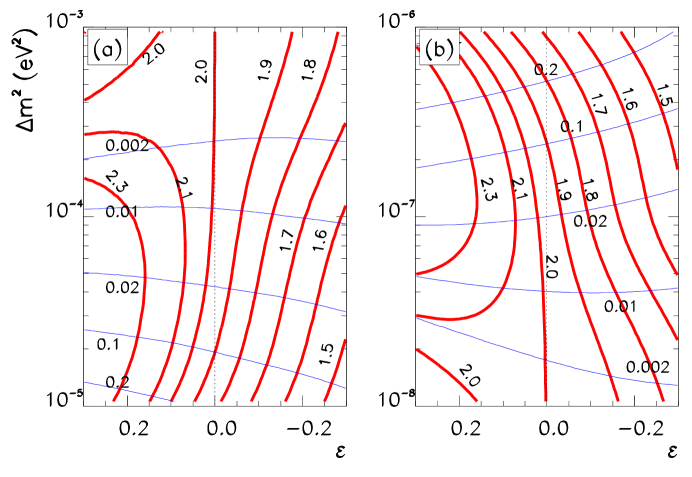
FIG. 15.: Iso–contours of [NC]/[CC] (thick lines) and of $A_{{\rm N-D}}^{{\rm CC}}$ for SNO (thin lines) in the $\Delta m^{2}-\epsilon$ plane in the (a) HIGH and (b) LOW regions.

D Borexino

The Borexino collaboration [40] will measure the total rate of ES events and search for time variations of the signal.

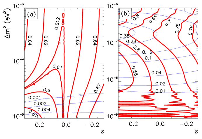
FIG. 16.: Iso–contours of the reduced rate (thick lines) and the Day–Night asymmetry (thin lines) predicted for the Borexino experiment in the $\Delta m^{2}-\epsilon$ plane for the QVO_L and HIGH (a), and LOW and QVO_S (b) regions.

In Fig. 16 we show iso-contours of the reduced rate $R_{Be}$ (suppression factor) and iso-contours of the Day-Night asymmetry in the $\Delta m^{2}-\epsilon$ plane. As discussed before for Super-Kamiokande and SNO, the Day-Night asymmetry is sensitive mainly to $\Delta m^{2}$ while the deviation from maximal mixing can be restricted by the rate for which we can write

$$R_{Be}=r_{Be}+(1-r_{Be})P~{},$$ (82)

where $r_{Be}\approx 0.24$ is the ratio of the $\nu_{\mu}-e$ to $\nu_{e}-e$ cross-sections for the beryllium neutrinos.

From Eq. (82) and Fig. 16 we observe the following behaviours:

(i) In the QVO_L region, the survival probability $P$ depends quadratically on $\epsilon$. We find $R_{Be}\sim 0.62$ with very weak $\epsilon$ dependence.

(ii) In the HIGH region, the transition between the quadratic and linear $\epsilon$ dependence occurs. For $\Delta m^{2}\sim 10^{-5}$ eV² the rate increases from 0.54 to 0.71 when $\epsilon$ decreases from $+0.3$ to $-0.3$. The Day–Night asymmetry is very small here.

(iii) In contrast, in the LOW region Borexino has higher sensitivity to the oscillation parameters. For maximal mixing, $R_{Be}$ is in the interval 0.65 - 0.70, and the asymmetry can be as large as 30%. The probability depends linearly on $\epsilon$, so that we get from Eq. (82)

$$\Delta\epsilon\sim\frac{2}{1-r_{Be}}\Delta R_{Be}.$$ (83)

Still, the sensitivity to $\epsilon$ is low but Borexino will play a crucial role in fixing $\Delta m^{2}$ and in particular by the measurement of the Day–Night asymmetry will be able to resolve the HIGH/LOW ambiguity which may remain after the measurements at Super–Kamiokande and SNO.

E LowNu Experiments

A new generation of experiments aiming at a high precision real time measurement of the low energy solar neutrino spectrum is now under study [41]. Some of them such us HELLAZ, HERON and SUPER–MuNu [42] intend to detect the elastic scattering of the electron neutrinos with the electrons of a gas and measure the recoil electron energy and its direction of emission. The proposed experiment LENS plans to detect the electron neutrino via its absorption in a heavy nuclear target with the subsequent emission of an electron and a delayed gamma emission [43]. The expected rates at those experiments for the proposed detector sizes are of the order of $\sim 1$–$10$ $pp$ neutrinos a day. Consequently, with a running time of two years they can reach a sensitivity of a few percent in the total neutrino rate at low energy, provided that they can achieve sufficient background rejection. This would allow the determination of $\epsilon$ with a similar precision of a few percent, in particular in the QVO_S, where SNO and Borexino cannot give much information due to their higher energy threshold.

Sensitivity to the oscillation parameters in the LMA region can also be achieved in experiments detecting low energy $\bar{\nu}_{e}$ fluxes from nuclear reactors (detection threshold is about $E_{th}=1.8$ MeV). The Borexino experiment, in addition to detecting solar neutrinos, aims to detect the diffuse fluxes from nuclear reactors in Europe, mainly in France and Germany, at an average distance $\sim 800$ km. The KamLAND experiment [39] aims at detecting the low energy diffuse $\bar{\nu}_{e}$ fluxes from reactors in Japan from an average distance of $\sim 200$ km. Both experiments can provide important information in discriminating between the HIGH and LOW solutions. However, they are expected to be very weakly sensitive to $\epsilon$. Given the short distances traveled by the neutrinos, matter effects are negligible for both experiments. Consequently, the survival probability for these experiments takes the vacuum form of Eqs. (27) and  (29) which depend only quadratically on $\epsilon$. With the expected achievable limits on the survival probability of about $\sim 10$–20%, a measurement of $|\epsilon|<0.3$ seems unfeasible.

VI Effects of the third neutrino

In the general case of three neutrino mixing when $|U_{e3}|\neq 0$ the definition of deviation from maximal mixing becomes ambiguous. Formally, maximal mixing of the $\nu_{e}$ in the three neutrino context can be defined as the equality $\theta_{12}=\pi/4$ where $\theta_{12}$ is the rotation angle in the plane of the first and second mass eigenstates. Phenomenologically, deviations from maximal mixing can be defined as a deviation of the averaged probability from 1/2 or a deviation of the depth of oscillations from 1.

Let us consider neutrino mass spectrum which explains also the atmospheric neutrino problem via (mainly) $\nu_{\mu}-\nu_{\tau}$ oscillations. This implies

$$|\Delta m^{2}_{\odot}|\equiv|\Delta m^{2}_{21}|\ll|\Delta m^{2}_{31}|\simeq|\Delta m^{2}_{32}|=|\Delta m^{2}_{{\rm atm}}|.$$ (84)

In this case (as far as solar neutrinos are concerned) the oscillations driven by $\Delta m^{2}_{\rm atm}$ can be averaged. This situation justifies our use of $\eta_{S}$ as defined in Eq. (22) and $\eta_{E}$ as defined in Eq. (33) in the calculation of the survival probabilities. We get the following expression for the survival probability [44]:

$$P_{ee}=(1-|U_{e3}|^{2})^{2}P_{2}+|U_{e3}|^{4}~{},$$ (85)

where $P_{2}=P(\Delta m^{2},\theta,V)$ is the two neutrino mixing survival probability determined by

$$\Delta m^{2}=\Delta m^{2}_{\odot},~{}~{}~{}~{}\tan\theta=|U_{e2}/U_{e1}|,~{}~{}~{}~{}~{}V=V_{0}(1-|U_{e3}|^{2}).$$ (86)

where $V_{0}$ is the matter potential $V_{0}=\sqrt{2}G_{F}\rho Y_{e}/m_{N}$. In principle we can define a parameter $\epsilon_{2}$ which describes the deviation from maximal mixing of $\theta$ defined in Eq. (86) similarly to the two neutrino parameters $\epsilon$ and $\theta_{ex}$ of Eq. (3). Then the deviation from maximal mixing in the three neutrino context will depend on the specific physical situation. If the mass splitting $\Delta m^{2}_{\odot}$ and the mixing angle $\theta$ induce vacuum oscillations, then $P_{2}\approx(1+\epsilon_{2}^{2})/2$ and Eq. (85) gives

$$P_{ee}\approx\frac{1}{2}+\frac{\epsilon_{2}^{2}}{2}-|U_{e3}|^{2}.$$ (87)

Thus one can define the deviation from maximal mixing in the three neutrino context in this case as $\epsilon_{3}^{v}=\epsilon_{2}^{2}-2|U_{e3}|^{2}$. Clearly, the three neutrino case reduces to the two neutrino case if

$$|U_{e3}|^{2}\ll\frac{1}{2}\epsilon_{2}^{2}.$$ (88)

Taking $|U_{e3}|^{2}$ at the level of the CHOOZ bound [16], $|U_{e3}|^{2}\sim 0.05$, Eq. (88) gives $|\epsilon_{2}|\gg 0.3$.

If $\Delta m^{2}_{\odot}$ and $\theta$ lead to the adiabatic conversion in matter, then $P_{2}\approx(1-\epsilon_{2})/2$ and Eq. (85) gives

$$P_{ee}\approx\frac{1}{2}-\frac{\epsilon_{2}}{2}-|U_{e3}|^{2}.$$ (89)

Here it is useful to characterize the deviation from maximal mixing through $\epsilon_{3}^{m}=\epsilon_{2}+2|U_{e3}|^{2}$. Corrections due to the third generation can be neglected provided that

$$|U_{e3}|^{2}\ll\frac{1}{2}\epsilon_{2}.$$ (90)

For $|U_{e3}|^{2}\sim 0.05$, Eq. (90) gives $\epsilon_{2}\gg 0.1$.

We have verified that, in the case of adiabatic transitions, the results of our calculations of the expected rates in the two-neutrino mixing scenario can be translated to a good approximation to the case of three-neutrino mixing with the simple replacement of $\epsilon_{2}$ with $\epsilon_{3}^{m}$. This applies, for instance, to the contours for the Ar–production rate in Fig. 6 and the predictions in Fig. 7 and Fig. 8 in the range $10^{-5}\gtrsim\Delta m^{2}$/eV${}^{2}\gtrsim 10^{-8}$. It also applies to the Ge–production rate in Fig. 13(b) and the corresponding predictions in Fig. 7 and Fig. 9(b) and 9(c). For the predictions of the SNO rates it can be used for Figs. 15 and 14 in the range $10^{-4}\gtrsim\Delta m^{2}$/eV${}^{2}\gtrsim 10^{-7}$, and for the predicted rates at Borexino in Fig. 16(b) for $\Delta m^{2}$/eV${}^{2}\gtrsim 5\times 10^{-9}$.

In the case of averaged vacuum oscillations (QVO_L) the results for the three-neutrino scenario can be read from the results presented here with the replacement of $\epsilon_{2}^{2}$ with $\epsilon_{3}^{v}$. For long wavelength oscillations (QVO_S and VO), the results for the three-neutrino scenario cannot be directly derived from our results. Thus our predictions in these regions only hold for very small values of the mixing angle $|U_{e3}|$, well below the present CHOOZ bound.

Concerning the value of $U_{e3}$, although certain improvement on the present CHOOZ bound may be expected from long baseline experiments, such as K2K and MINOS [45], their final sensitivity is still unclear as it depends on their capability of discriminating against the $\nu_{e}$ beam contamination. Ultimate sensitivity can be achieved at experiments performed with neutrino beams from muon-storage rings at the so-called neutrino factories [46].

VII Maximal mixing and other experiments

In the previous sections we have concentrated on effects in the solar neutrinos. Mixing of the electron neutrino can be probed in a number of other experiments.

A Atmospheric neutrinos

Maximal and near–maximal mixing of the electron neutrinos can be probed in the atmospheric neutrino studies. The oscillations in the Earth matter with parameters from the LMA or HIGH regions can give an observable effect in the $e$-like events. The electron neutrino flux at the detector [47, 48, 49, 50] can be written as [50]

$$F_{e}=F_{e}^{0}\left[1+P_{e\mu}(r\cos^{2}\theta_{23}-1)\right]~{},$$ (91)

where $r\equiv F_{\mu}^{0}/F_{e}^{0}$ is the ratio of the original electron and muon neutrino fluxes, $P_{e\mu}=P(\Delta m_{\odot}^{2},\epsilon_{2})$ is the two neutrino transition probability, and $\theta_{23}$ is the $\nu_{\mu}-\nu_{\tau}$ mixing responsible for the dominant mode of the atmospheric neutrino oscillations. The transition probability can be of order one at $\Delta m^{2}>3\times 10^{-4}$ eV². It decreases fast with $\Delta m^{2}/E$ due to matter suppression of the mixing. Thus the biggest effect is expected in the low energy (sub-GeV) events sample. Notice that the probability $P_{e\mu}$ enters in Eq. (91) with a “screening factor” $(r\cos^{2}\theta_{23}-1)$ which turns out to be small. Indeed, for the sub-GeV sample $r\approx 2$ and the screening factor is exactly zero for maximal mixing in the atmospheric neutrinos [50, 51]. The factor equals approximately $\cos 2\theta_{23}$, so that for $\sin^{2}2\theta_{23}=0.95$ we get about 0.22.

For $\theta_{23}<\pi/4$ the oscillations lead to the excess of the $e$-like events. Indeed some excess is hinted by the SK data. The excess can be defined as $N_{e}/N_{e}^{0}-1$, where $N_{e}$ and $N_{e}^{0}$ are the numbers of events with and without oscillations. This excess can be written in a matter dominant regime of oscillations ($\eta_{E}\ll 1$) as

$$\frac{N_{e}}{N_{e}^{0}}-1\approx\cos 2\theta_{23}\eta_{E}^{2}(1-\epsilon_{2}\,\eta_{E}),$$ (92)

where $\epsilon_{2}$ was defined below Eq. (86). The excess depends on $\epsilon_{2}$ linearly and it increases with $\eta_{E}$. However it is even more sensitive to deviations of $\theta_{23}$ from the maximal mixing value. For $\Delta m^{2}_{21}=10^{-4}$ eV² and $\sin^{2}2\theta_{23}=0.95$ the excess reaches about 3% and the dependence on $\epsilon$ is weak. For $\Delta m^{2}_{21}=2\cdot 10^{-4}$ eV² and the same $\theta_{23}$, we find the excess about 4.5 %. Significant dependence on $\epsilon$ appears for $\Delta m^{2}_{12}=3\times 10^{-4}$ eV². However, it is unlikely given the size of the effect that atmospheric neutrino data will give any significant information on the value of $\epsilon_{2}$.

B Supernova neutrinos

Maximal or near–maximal mixing of the electron neutrinos will significantly modify properties of neutrino bursts from supernovae. The effects depend crucially on features of the whole neutrino mass spectrum and in particular on the value of $U_{e3}$ and whether the mass hierarchy is normal ($\Delta m^{2}_{31}>0$) or inverted ($\Delta m^{2}_{31}<0$). Let us summarize here the main results (for more details see [52] and references therein).

All oscillation and conversion effects in supernova neutrinos are determined by the total survival probability of the electron neutrinos which in this subsection we will write as $p$, and total survival probability of the electron antineutrinos, $\bar{p}$. (This property is related to the fact that the original spectra of the muon and the tau neutrinos are identical and that the muon and tau neutrinos cannot be distinguished at the detection point).

The probabilities should include the effects of propagation inside the star, on the way to the Earth and inside the Earth. Using the probabilities $p$ and $\bar{p}$, one can write the fluxes of the electron neutrinos, $F_{e}$, and electron antineutrinos, $F_{\bar{e}}$, at the detector in terms of the original electron (anti)neutrino fluxes, $F_{e}^{0}$ and $F_{\bar{e}}^{0}$, and the non-electron neutrino flux $F_{x}^{0}\equiv F_{\mu}^{0}=F_{\tau}^{0}=F_{\bar{\mu}}^{0}=F_{\bar{\tau}}^{0}$:

$$F_{e}=p\cdot F_{e}^{0}+(1-p)\cdot F_{x}^{0}~{},~{}~{}~{}~{}F_{\bar{e}}=\bar{p}\cdot F_{\bar{e}}^{0}+(1-\bar{p})\cdot F_{x}^{0}~{}.$$ (93)

In general, $p$, and $\bar{p}$ depend on the neutrino energy.

Let us summarize the results for specific neutrino mass and flavor spectra.

1) If $|U_{e3}|^{2}>3\times 10^{-4}$ the conversion in the resonance related to the largest (atmospheric) splitting ($\Delta m^{2}_{31}$) will be completely adiabatic and the final effect depends on the type of mass hierarchy. In the case of normal hierarchy ($\nu_{3}$ is the heaviest state) the resonance conversion occurs in the neutrino channel and for the survival probability we get

$$p\approx|U_{e3}|^{2}\ll 1.$$ (94)

This probability is practically independent of the properties (mass, flavour) of the first and second mass eigenstates. In particular, there is no sensitivity to $\epsilon$ and no Earth matter effect is expected for neutrinos.

In contrast, the antineutrino channels will not be affected by the high resonance and $\bar{p}$ will be determined by physics of the two light levels.

For parameters in the HIGH and LOW regions, the neutrino propagation in the star is adiabatic, so that the survival probability in the star equals

$$\bar{p}\approx\cos^{2}\theta_{12}=\frac{1}{2}(1+\epsilon).$$ (95)

This probability can be further modified due to oscillations in the matter of the Earth. Thus, we expect the following consequences: (i) disappearance of the $\nu_{e}$ neutronization peak; (ii) hard $\nu_{e}$ spectrum (coinciding with the original $\nu_{\mu}$) spectrum at the cooling stage:

$$F_{e}\approx F_{x}^{0}~{};$$ (96)

(iii) composite $\bar{\nu}_{e}$ spectrum:

$$F_{\bar{e}}=\frac{1}{2}(F_{\bar{e}}^{0}+F_{x}^{0})-\frac{\epsilon}{2}(F_{x}^{0}-F_{\bar{e}}^{0});$$ (97)

(iv) strong Earth matter effect (which leads to different signals at various detectors). For the HIGH mass range, the Earth effect is maximal in the high energy part of the spectrum, $E>20$ MeV, whereas for the LOW solution the largest effect is in the low energy part.

According to Eq. (97), the $\epsilon$-dependent term is proportional to the difference of the original fluxes. Thus due to the uncertainties in the predicticted fluxes it will be difficult to measure $\epsilon$. In order to reduce the theoretical uncertainty, one could in principle compare numbers of $\nu_{e}$ and $\bar{\nu}_{e}$ events at large $E$ which are determined by, respectively, $F_{x}^{0}$ and $F_{x}^{0}(1-\epsilon)/2$ and are proportional to the same flux.

For parameters of the two light states in the VO region, the neutrino propagation in the star is non-adiabatic, so that the survival probability can be writen as

$$\bar{p}\approx(1-P_{c})\cos^{2}\theta_{12}+P_{c}\sin^{2}\theta_{12}=\frac{1}{2}+\epsilon\left(\frac{1}{2}-P_{c}\right),$$ (98)

where the jump probability $P_{c}$ depends on the details of the density profile in the outer regions of the star and cannot be reliably predicted. Practically, the probability should lie between the adiabatic value (95) and the pure vacuum oscillation expression $p=(1+\epsilon^{2})/2$.

In the case of inverted mass hierarchy the sensitivity to $\epsilon$ appears in the neutrino channel and neutrinos and antineutrinos interchange their roles. Now the resonance is in the antineutrino channel so that

$$\bar{p}\approx|U_{e3}|^{2}\ll 1,$$ (99)

and the oscillations in the neutrino channels will be determined by physics of the two light levels. For parameters from the HIGH and LOW regions the propagation in the star is adiabatic and

$$p\approx\sin^{2}\theta_{12}=\frac{1}{2}(1+\epsilon).$$ (100)

Moreover, Earth matter effects are expected for neutrinos. For the VO region we find, similarly to Eq. (98),

$$p\approx\frac{1}{2}-\epsilon\left(\frac{1}{2}-P_{c}\right).$$ (101)

In this inverted scheme we predict: (i) partial disappearance of the $\nu_{e}$ neutronization peak; (ii) hard spectrum of the electron antineutrinos:

$$F_{\bar{e}}\approx F_{x}^{0}~{};$$ (102)

(iii) composite $\nu_{e}$ spectrum:

$$F_{e}=\frac{1}{2}(F_{e}^{0}+F_{x}^{0})+\frac{\epsilon}{2}(F_{x}^{0}-F_{e}^{0});$$ (103)

(iv) Earth matter effects are expected in the neutrino channel only.

2) If $|U_{e3}|^{2}<3\times 10^{-6}$, the effect of the third neutrino can be neglected: in the resonance channel the transition driven by $U_{e3}$ is strongly non-adiabatic, and in the non-resonance channel the mixing is always very small. In this case the problem is reduced to transitions in two level system with parameters determined by $\Delta m^{2}_{21}=\Delta m^{2}_{\odot}$ and $\epsilon$. As a result both neutrino and antineutrino channels turn out to be sensitive to $\epsilon$. The effects include those considered above both for normal and inverted mass hierarchy.

For HIGH and LOW regions of parameters the propagation proceeds adiabaticaly, and for the survival probabilities we get the expressions given in (95) and (100). Correspondingly, neutrino and antineutrino spectra will be given by Eq. (97) and (103). Thus we predict that both neutrino and antineutrino spectra will be composite, consisting of nearly equal admixture of the soft and hard components. In the high energy part where effects of the soft components can be neglected we get from Eqs. (97) and (103):

$$\frac{F_{e}}{F_{\bar{e}}}\sim 1+2\epsilon.$$ (104)

That is, larger $\nu_{e}$ signal (as compared with $\bar{\nu_{e}}$) is expected for $\epsilon>0$ and smaller for $\epsilon<0$. Also Earth matter effect is expected in both neutrino and antineutrino channels.

3) If $|U_{e3}|^{2}$ is in the intermediate region, $3\times 10^{-6}-3\times 10^{-4}$, the adiabaticity in high mass resonance is partially violated and we expect some intermediate situation between those described in 1) and 2). In particular, both $\nu_{e}$ and $\bar{\nu}_{e}$ spectra will be composite, however admixtures of the soft and hard components will be unequal, etc..

To conclude, one expects strong influence of maximal and near–maximal mixing on the properties of the neutrino bursts. However, the uncertainties in the predicted neutrino spectra will make it difficult to obtain high sensitivity to $\epsilon$.

Notice also that the analysis of the SN1987A data gives the 99% CL bound on $p>0.65$. This would correspond to $\bar{p}>0.3$ [53]. Some recent calculations show that the difference between $\bar{\nu}_{e}$ and $\bar{\nu}_{\mu}$ original spectra can be rather small, which would somewhat relax the above bound.

C Neutrinoless double beta decay

The effective Majorana mass of the electron neutrino $m_{ee}$ relevant for the neutrinoless double beta decay is sensitive to the distribution of the electron neutrino flavor in the mass eigenstates (see [54] for recent discussion). The contribution to the effective mass $m_{ee}$ from the two mass eigenstates responsible for the solar neutrino conversion can be written in terms of the oscillation parameters as

$$m_{ee}=\frac{1}{2}\left|m_{1}(1+\epsilon)+\sqrt{m_{1}^{2}+\Delta m_{\odot}^{2}}(1-\epsilon)e^{i\phi_{12}}\right|,$$ (105)

where $m_{1}$ is the mass of the first eigenstate and $\phi_{12}$ is the relative phase of the first and the second mass eigenvalues. In the case of strong mass hierarchy, $m_{1}^{2}\ll\Delta m_{\odot}^{2}$ we get from Eq. (105)

$$m_{ee}\approx\frac{1}{2}\sqrt{\Delta m_{\odot}^{2}}(1-\epsilon).$$ (106)

According to this equation in the HIGH region the effective mass can be as big as $(1-2)\times 10^{-2}$ eV which can be probed at the next generation of the double beta decay experiments [55]. Notice that the contribution from the third mass eigenstate is strongly restricted by present experimental bound $m_{ee}<2\times 10^{-3}$ eV.

Although the dependence of $m_{ee}$ on $\epsilon$ is rather strong, it will be difficult to measure $\epsilon$ due to the uncertainties in the nuclear matrix elements. Eq. (106) can be considered as a test equation: if the measured values of $m_{ee}$, $\epsilon$ and $\Delta m_{\odot}^{2}$ indeed satisfy this equation (within experimental and theoretical uncertainties) it will testify for the validity of whole scheme.

In the case of strong mass degeneracy, $m_{1}^{2}\gg\Delta m_{\odot}^{2}$ we get

$$m_{ee}\approx\frac{1}{2}m_{1}\left|(1+\epsilon)+(1-\epsilon)e^{i\phi_{12}}\right|,$$ (107)

where both non-oscillation parameters $m_{1}$ and $\phi_{12}$ are unknown. For $\phi_{12}=\pi$ and $(0)$ the mass equals $m_{ee}=m_{1}\epsilon$ $(m_{1})$, so that $\epsilon$ determines the lower bound on $m_{ee}$. If $m_{ee}$ and $\epsilon$ are measured, the above equalities will determine the upper bound and the lower bounds on the absolute scale of the neutrinos mass: $m_{ee}<m_{1}<m_{ee}/\epsilon$.

In the case of inverted mass hierarchy the two states responsible for the solar neutrino conversion are degenerate: $m_{1}\approx m_{2}\approx\sqrt{\Delta m^{2}_{\rm atm}}$ and the effective majorana mass can be written as

$$m_{ee}\approx\frac{1}{2}\sqrt{\Delta m^{2}_{\rm atm}}\left|(1+\epsilon)+(1-\epsilon)e^{i\phi_{12}}\right|.$$ (108)

In this case the measurement of $\epsilon$ will allow us to determine the phase $\phi_{12}$. According to Eq. (108), $\sqrt{\Delta m^{2}_{\rm atm}}\epsilon<m_{ee}<\sqrt{\Delta m^{2}_{\rm atm}}$ which can be used as a test inequality for a given scheme.

Thus measurements of $\epsilon$ in the oscillation experiments will allow to determine or restrict the effective mass $m_{ee}$ in the context of certain schemes of neutrino masses and mixing.

VIII Conclusions

In this work we have explored the phenomenological consequences of (near–)maximal mixing of electron neutrinos with other standard neutrinos. The possibility of such maximal or near–maximal lepton mixing constitutes an intriguing challenge for fundamental theories of flavour. Our aim was twofold. First we have formulated the present status of maximal mixing of $\nu_{e}$ in the light of existing experimental data from solar neutrino experiments. Second we have explored the best ways to measure deviations from such maximal mixing at future experiments.

We show in Sec. II that both probabilities and observables depend on $\epsilon$ quadratically in the regions of $\Delta m^{2}$ where the effects are due to vacuum oscillations, and they depend on $\epsilon$ linearly when matter effects dominate. Consequently, for $|\epsilon|\ll 1$ the highest sensitivity to deviation from maximal mixing can be achieved in the $\Delta m^{2}$ ranges of the MSW effect.

The results of a global fit to the existing solar neutrino data are presented in Sec. III and summarized in Figs. 2 $-$5. From this analysis we find that values of the mixing parameter $|\epsilon|\equiv|1-2\sin^{2}\theta|<0.3$ are allowed at 99% or lower CL for $\Delta m^{2}\mathrel{\hbox to0.0pt{\lower 4.0pt\hbox{\hskip 1.0pt$\sim$}\hss}\raise 1.0pt\hbox{$>$}}1.5\times 10^{-5}$ eV² (which contains the HIGH and QVO_L regions) and for $4\times 10^{-10}$ eV${}^{2}\mathrel{\hbox to0.0pt{\lower 4.0pt\hbox{\hskip 1.0pt$\sim$}\hss}\raise 1.0pt\hbox{$<$}}\Delta m^{2}\mathrel{\hbox to0.0pt{\lower 4.0pt\hbox{\hskip 1.0pt$\sim$}\hss}\raise 1.0pt\hbox{$<$}}2\times 10^{-7}$ eV² (which contains the defined LOW, QVO_S and upper VAC_L regions).

The role of the individual existing experiments on the determination of these regions is discussed in Sec. IV. We conclude that the present sensitivity to the mixing angle arises from the measurements of total event rates. The present data from Homestake experiment in Ar–production rate gives the strongest constraint on maximal or near–maximal mixing as it favours a significant deviation from $\epsilon=0$. This conclusion is independent of the existing theoretical uncertainty on the boron flux as discussed in Sec. IV B. On the other hand the measurement of the zenith angle dependence and the recoil electron energy spectrum are important in the determination of the allowed mass ranges but are very weakly sensitive to deviation from maximal mixing. With the present existing sensitivity all values of $|\epsilon|<0.3$ are allowed within 4$\sigma$.

In Sec. V we have discussed the ways to improve our knowledge on deviations from maximal mixing at future experiments. We concentrate on observables which are SSM (or at least boron flux) independent. In order to determine both the mass and the mixing we study pairs of observables. First we have looked at the maximal sensitivity which may be achievable on the presently running experiments GNO and Super–Kamiokande. In principle the measurement of the Ge–production rate at GNO and the Day–Night asymmetry at Super–Kamiokande and SNO can give crossed information on the oscillation parameters in the matter conversion region. In practice, however, the expected sensitivity is not enough to substantially improve the present knowledge on $\Delta m^{2}$ and $\epsilon$. The role of SNO and Borexino experiments is discussed in Secs. V C and V D. We show that with the expected theoretical and statistical uncertainty the most sensitive observable to the mixing angle is the rate [NC]/[CC] measurable at SNO. For instance, a measurement yielding [NC]/[CC] $\sim 2\times(1\pm 0.04)$ and $A_{{\rm N-D}}^{{\rm CC}}\sim 0.1\times(1\pm 0.3)$ will determine $\epsilon$ to an accuracy of order $\Delta\epsilon\sim 0.07$. There exist however an ambiguity on the allowed mass range between HIGH and LOW regions. We show that the LOW/HIGH ambiguity can be resolved by the measurement of the Day–Night asymmetry at Borexino experiment which is sensitive to strong Earth regeneration effect in the LOW region or by the detection of oscillations in long baseline reactor experiments such as KamLand. However no substantial improvement on the knowledge of $\epsilon$ is expected neither from Borexino nor from the new generation of low energy experiments either with solar or reactor neutrinos.

- [1] Z. Maki, M. Nakagawa and S. Sakata, Prog. Theo. Phys. 28, 870 (1962).
- [2] Super–Kamiokande Collaboration, Y. Fukuda et al., Phys. Rev. Lett. 81, 1562 (1998) [hep-ex/9807003].
- [3] For a recent analysis see N. Fornengo, M. C. Gonzalez-Garcia and J. W. F. Valle, Nucl. Phys. B580, 58 (2000) [hep-ph/0002147].
- [4] M. C. Gonzalez-Garcia, P. C. de Holanda, C. Peña-Garay, J. W. F. Valle, Nucl. Phys. B573, 3 (2000) [hep-ph/9906469]; M. C. Gonzalez-Garcia, C. Peña-Garay, hep-ph/0009041.
- [5] M. C. Gonzalez-Garcia, C. Peña-Garay, Phys. Rev. D62, 031301 (2000) [hep-ph/0002186].
- [6] G. L. Fogli, E. Lisi, A. Maronne and G. Scioscia, Phys. Rev. D59, 033001 (1999) [hep-ph/9808205].
- [7] C. Giunti, M. C. Gonzalez-Garcia, C. Peña-Garay, Phys. Rev. D62, 013005 (2000) [hep-ph/0001101].
- [8] J. N. Bahcall, P. I. Krastev, A. Yu. Smirnov, Phys. Rev. D60, 093001 (1999) [hep-ph/9905220].
- [9] J. N. Bahcall, P. I. Krastev, A. Yu. Smirnov, Phys. Lett. B477, 401 (2000) [hep-ph/9911248].
- [10] A. de Gouvea, A. Friedland and H. Murayama, hep-ph/0002064.
- [11] Y. Nir, JHEP 0006, 039 (2000) [hep-ph/0002168].
- [12] Y. Grossman and Y. Nir, Nucl. Phys. B448, 30 (1995) [hep-ph/9502418].
- [13] Y. Grossman, Y. Nir and Y. Shadmi, JHEP 9810, 007 (1998) [hep-ph/9808355].
- [14] R. Barbieri, L.J. Hall, D. Smith, A. Strumia and N. Weiner, JHEP 9812, 017 (1998) [hep-ph/9807235].
- [15] V. Barger, S. Pakvasa, T. J. Weiler and K. Whisnant, Phys. Lett. B437, 107 (1998) [hep-ph/9806387].
- [16] CHOOZ collaboration, M. Apollonio et al., Phys. Lett. B420, 397 (1998) [hep-ex/9711002]; Phys. Lett. B466, 415 (1999) [hep-ex/9907037].
- [17] V. Barger, T. J. Weiler and K. Whishnant, Phys. Lett. B440, 1 (1998) [hep-ph/9807319].
- [18] J. Pantaleone, Phys. Lett. B251, 618 (1990); S. Pakvasa and J. Pantaleone, Phys. Rev. Lett. 65, 2479 (1990)
- [19] G. L. Fogli, E. Lisi, D. Montanino and A. Palazzo, hep-ph/0005261.
- [20] A. Friedland, Phys. Rev. Lett. 85, 936 (2000) [hep-ph/0002063].
- [21] http://www.sns.ias.edu/~jnb/SNdata/Export/BP2000; J. N. Bahcall, S. Basu and M. H. Pinsonneault, Astrophys. J. 529, 1084 (2000).
- [22] A. M. Dziewonski and D. L. Anderson, Phys. Earth Planet. Inter. 25, 297 (1981).
- [23] S. T. Petcov, Phys. Lett. B200, 373 (1988).
- [24] P. I. Krastev and S. T. Petcov, Phys. Lett. B207, 64 (1988) 64.
- [25] A. de Gouvea, A. Friedland and H. Murayama, hep-ph/9910286; Phys. Rev. D60, 093011 (1999);
- [26] P.C. de Holanda, C. Pena-Garay, M.C. Gonzalez-Garcia, J.W.F. Valle, Phys. Rev. D60, 093010 (1999) [hep-ph/9903473].
- [27] G. L. Fogli, E. Lisi, D. Montanino and A. Palazzo, Phys. Rev. D61, 073009 (2000) [hep-ph/9910387].
- [28] B. T. Cleveland et al., Astrophys. J. 496, 505 (1998); R. Davis, Prog. Part. Nucl. Phys. 32, 13 (1994).
- [29] SAGE Collaboration, J. N. Abdurashitov et al., Phys. Rev. C60, 055801 (1999); Talk by V. Gavrin at XIX International Conference on Neutrino Physics and Astrophysics, http://ALUMNI.LAURENTIAN.CA/www/physics/nu2000.
- [30] GALLEX Collaboration, W. Hampel et al., Phys. Lett. B447, 127 (1999).
- [31] Talk by E. Belloti at XIX International Conference on Neutrino Physics and Astrophysics, http://ALUMNI.LAURENTIAN.CA/www/physics/nu2000; T. A. Kirsten, Nucl. Phys. Proc. Suppl. 77, 26 (1999).
- [32] Super–Kamiokande Collaboration, Y. Fukuda et al., Phys. Rev. Lett. 81, 1158 (1998); Erratum 81, 4279 (1998); 82, 1810 (1999); 82, 2430 (1999); Y. Suzuki, Nucl. Phys. B (Proc. Suppl.) 77, 35 (1999).
- [33] Talk by Y. Suzuki at XIX International Conference on Neutrino Physics and Astrophysics, http://ALUMNI.LAURENTIAN.CA/www/physics/nu2000.
- [34] Palo Verde collaboration, F.Boehm et al., hep-ex/0003022.
- [35] J. N. Bahcall, S. Basu and M. H. Pinsonneault, Phys. Lett. B433, 1 (1998).
- [36] A. B. McDonald, Nucl. Phys. B (Proc. Suppl.) 77, 43 (1999); SNO Collaboration, Physics in Canada 48, 112 (1992); SNO Collaboration, nucl-ex/9910016.
- [37] J. N. Bahcall and E. Lisi, Phys. Rev. D 54, 5417 (1996); K. Kubodera and S. Nozawa, Int. J. Mod. Phys. E 3, 101 (1994); S. Ying, W. C. Haxton and E. M. Henley, Phys. Rev. C 45, 1982 (1992); S. D. Ellis and J. N. Bahcall, Nucl. Phys. A 114, 636 (1986).
- [38] J. N. Bahcall, P. I. Krastev, A. Yu. Smirnov, hep-ph/0002293; hep-ph/0006078.
- [39] For a recent status report see A. Suzuki, Nucl. Phys. B (Proc. Suppl.) 77, 171 (1999).
- [40] L. Oberauer, Nucl. Phys. (Proc. Suppl.) 77, 48 (1999).
- [41] For present status see the proceedings of the workshop LowNu: Solar Neutrino Experiments below 1 MeV, http://www-sk.iccr.u-tokyo.ac.jp/lownu/index.html.
- [42] A. de Bellfon for the HELLAZ collaboration, Nucl. Phys. (Proc. Suppl.) B70, 386 (1999); R.E. Lanou, H.J. Maris, T. More, F.S. Porter and G.M. Seidel, J. Low Temp. Phys. 93, 785 (1993); C. Arpesella, C. Broggini, and C. Cattadori, Ast. Phys. 4, 333 (1996).
- [43] R.S. Raghavan, Phys. Rev. Lett 78, 3618 (1997).
- [44] Chong-Sa Lim, BNL-39675, Feb 1987, BNL Neutrino Workshop 1987:111.
- [45] M.C. Gonzalez-Garcia and C. Peña-Garay, hep-ph/0001129.
- [46] V. Barger et al., Phys. Rev. D62, 013004 (2000); A. Cervera et al., Nucl. Phys. B579, 17 (2000).
- [47] G. L. Fogli, E. Lisi, D. Montanino and A. Palazzo, Phys. Rev. D62, 013002 (2000).
- [48] O. Yasuda, hep-ph/9602342; hep-ph/9707564.
- [49] C. W. Kim and U. W. Lee, Phys. Lett. B444, 204 (1998).
- [50] O. L. G. Peres and A. Yu. Smirnov, Phys. Lett. B456, 204 (1999).
- [51] I. Stancu and D. V. Ahluwalia, Phys. Lett. B460, 431 (1999).
- [52] A.S. Dighe and A. Yu. Smirnov, Phys. Rev. D62, 033007 (2000) [hep-ph/9907423].
- [53] A. Yu. Smirnov, D. N. Spergel and J. N. Bahcall, Phys. Rev. D49, 1389 (1994).
- [54] S. T. Petcov and A. Yu. Smirnov, Phys. Lett. B322, 109 (1994); H. Minakata and O. Yasuda, Nucl. Phys. B523, 597 (1998); F. Vissani, hep-ph/9904349; R. Adhikari and G. Rajasekaran, Phys. Rev. D61, 031301 (2000); S. M. Bilenky, C. Giunti, W Grimus, B. Kayser and S. T. Petcov, Phys. Lett. B465, 193 (1999); H. V. Klapdor-Kleingrothaus, H. Pas and A. Yu. Smirnov, hep-ph/0003219.
- [55] V. Lobashev et al., Phys. Lett. B460, 227 (1999); Ch. Weinheimer et al., Phys. Lett. B460, 219 (1999).