hep-ph/0007226

CERN-TH/2000-125

July 2000

Large Dimensions and String Physics in Future Colliders

I. Antoniadis and K. Benakli

CERN Theory Division CH-1211, Genève 23, Switzerland

ABSTRACT

We review the status of low-scale string theories and large extra-dimensions. After an overview on different string realizations, we discuss some of the main important problems and we summarize present bounds on the size of possible extra-dimensions from collider experiments.

1.   Introduction
2.   Hiding extra dimensions
2.1  Compactification on tori and Kaluza-Klein states
2.2  Orbifolds and localized states
2.3  Early motivation for large extra dimensions
3.   Low-scale strings
3.1  Type I/I^′ string theory and D-branes
3.2  Type II theories
3.3  Heterotic string and M-theory on $S^{1}/Z_{2}$“$\times$”Calabi-Yau
3.4  Relation between Type I/I^′ and Type II with heterotic strings
4.   Theoretical implications
4.1  U.V./I.R. correspondance
4.2  Unification
4.3  Supersymmetry breaking and scales hierarchy
4.4  Electroweak symmetry breaking in TeV-scale strings
5.  Scenarios for studies of experimental constraints
6.  Extra-dimensions along the world brane: KK excitations of gauge bosons
6.1  Production at $e^{+}e^{-}$ colliders
6.2  Production at hadron colliders
6.3  High precision data low-energy bounds
6.4  One extra dimension for other cases
6.5  More than one extra dimension
7.  Extra-dimensions transverse to the world brane: KK excitations of gravitons
7.1  Signals from missing energy experiments
7.2  Gravity modification and sub-millimeter forces
8.  Dimension-eight operators and limits on the string scale
9.  Conclusions
References

1 Introduction

In how many dimensions do we live? Could they be more than the four we are aware of? If so, why don’t we see the other dimensions? Is there a way to detect them?. While the possibility of extra-dimensions has been considered by physicists for long time, a compelling reason for their existence has arisen with string theory. It seems that a quantum theory of gravity requires that we live in more than four dimensions, probably in ten or eleven dimensions. The remaining (space-like) six or seven dimensions are hidden to us: observed particles do not propagate in them. The theory does not tell us yet why four and only four have been accessible to us. However, it predicts that this is only a low-energy effect: with increasing energy, particles which propagate in a higher dimensional space could be produced. What is the value of the needed high energy scale? could it be just close by, at reach of near future experiments?

Another scale which appears in our attempts to answer the previous questions is related to the extended nature of fundamental objects. It is the scale at which internal degrees of freedom are excited. In string theory this scale $M_{s}$ is related to the string tension and sets the mass of the first heavy oscillation mode. The point-like behavior of known particles as observed at present colliders allows to conclude that $M_{s}$ has to be higher than a few hundred GeV. However to answer the question of what energies should be reached before starting to probe this substructure of the “fundamental particles”, more precise determination of experimental lower bounds on $M_{s}$ and understanding the assumptions behind them is needed.

It is the aim of this review as to provide a short summary of the present status of research on extra-dimensions and string-like sub-structure of matter.

2 Hiding Extra-Dimensions

2.1 Compactification on Tori and Kaluza-Klein states

There is a simple and elegant way to hide the extra-dimensions: compactification. It is simple because it relies on an elementary observation. Suppose that the extra-dimensions form, at each point of our four-dimensional space, a $D$-dimensional torus of volume $(2\pi)^{D}R_{1}R_{2}\cdots R_{D}$. The $(4+D)$-dimensional Poincare invariance is replaced by a four-dimensional one times the symmetry group of the $D$-dimensional space which contains translations along the $D$ extra directions. The $(4+D)$-dimensional momentum satisfies the mass-shell condition $P_{(4+D)}^{2}=p_{0}^{2}-p_{1}^{2}-p_{2}^{2}-p_{3}^{2}-\sum_{i}p_{i}^{2}=m_{0}^{2}$ and looks from the four-dimensional point of view as a (squared) mass $M^{2}_{KK}=p_{0}^{2}-p_{1}^{2}-p_{2}^{2}-p_{3}^{2}=m_{0}^{2}+\sum_{i}p_{i}^{2}$. Assuming periodicity of the wave functions along each compact direction, one has $p_{i}=n_{i}/R_{i}$ which leads to:

$$M^{2}_{KK}\equiv M^{2}_{\vec{n}}=m_{0}^{2}+\frac{n_{1}^{2}}{R_{1}^{2}}+\frac{n_{2}^{2}}{R_{2}^{2}}+\cdots+\frac{n_{D}^{2}}{R_{D}^{2}}\,,$$ (1)

with $m_{0}$ the higher-dimensional mass and $n_{i}$ non-negative integers. The states with $\sum_{i}n_{i}\neq 0$ are called Kaluza-Klein (KK) states. It is clear that getting aware of the $i$th extra-dimension would require experiments that probe at least an energy of the order of $min(1/R_{i})$ with sizable couplings of the KK states to four-dimensional matter.

Let us discuss further some properties of the KK states that will be useful for us below. We parametrise the “internal” $D$-dimensional box by $y_{i}\in[-\pi R_{i},\pi R_{i}]$, $i=1,\cdots,D$ while the four-dimensional Minkowski spacetime is spanned by the coordinates $x^{\mu}$, $\mu=0,\cdots,3$. It is useful to choose for the KK wave functions the basis:

$$\Phi^{\alpha}_{{\vec{n}},{\vec{e}}}(x^{\mu},y_{i})=\Phi^{\alpha}(x^{\mu})\,\prod_{i}\left[(1-e_{i})\cos(\frac{n_{i}y_{i}}{R_{i}})+e_{i}\sin(\frac{n_{i}y_{i}}{R_{i}})\right]\,,$$ (2)

where the vector ${\vec{n}}=(n_{1},n_{2},\cdots,n_{D})$ gives the energy of the state following Eq. (1) while ${\vec{e}}=(e_{1},\cdots,e_{D})$ with $e_{i}=0$ or 1 corresponds to a choice of cosine or sine dependence in the coordinate $y_{i}$, respectively. The index ${\alpha}$ refers to other quantum numbers of $\Phi$.

2.2 Orbifolds and localized states

The simplest example of the models we will be using for getting experimental bounds are obtained by gauging the $Z_{2}$ parity: $y_{i}\rightarrow-y_{i}\,{\rm mod}\,2\pi R_{i}$. This leads to compactification on segments of size $\pi R_{i}$. In general, the consistency of this “orbifold” projection implies that the $Z_{2}$ space parity should be associated with a $Z_{2}$ action on the internal quantum numbers $\alpha$ of $\Phi$. As a result one has the following properties:

• Only states invariant under this $Z_{2}$ are kept while the others are projected out. There are two classes of states left in the theory: those for which $\Phi^{(even)}(x^{\mu})$ is even under the $Z_{2}$ action and $e_{i}=0$ and those for which $\Phi^{(odd)}(x^{\mu})$ is odd and $e_{i}=1$. It is important to notice that the latter are not present as light four-dimensional states i.e. they have $\sum_{i}n_{i}\neq 0$ and thus always correspond to higher KK states.

• At the boundaries $y_{i}=0,\pi R$ fixed by the $Z_{2}$ action, new states $\Phi^{(loc)}(x^{\mu})$, have to be included. These “twisted” states are localized at the fixed points. They can not propagate in the extra-dimension and thus have no KK excitations.

• The odd bulk states $\Phi^{(odd)}(x^{\mu})$ ($e_{i}=1$) have a wave function which vanishes (the $\sin(\frac{n_{i}y_{i}}{R_{i}})$ in Eq. (1 ) at the boundaries. Their coupling to localized states involves a derivative along $y_{i}$. For example three boson interactions of the form $\partial_{i}\phi^{(odd))}\phi^{(loc)}\phi^{(loc)}$ can be non-vanishing.

• The even states, in contrast, can have non-derivative couplings to localized states. The gauge couplings for instance are given by:

  $$g_{n}={\sqrt{2}}\delta^{-{|\vec{\frac{n}{R}}|^{2}}/{M_{s}^{2}}}g$$ (3)

  where $\delta>1$ is a model dependent number ($\delta=4$ in the case of $Z_{2}$). The ${\sqrt{2}}$ comes from the relative normalization of $\cos(\frac{n_{i}y_{i}}{R_{i}})$ wave function with respect to the zero mode while the exponential damping is a result of tree-level string computations that we do not present here.

  The exchange of KK states gives rise to an effective four-fermion operator:

  $${\bar{\psi}_{1}}{\psi_{2}}{\bar{\psi}_{3}}{\psi_{4}}\sum_{|\vec{n}|}\frac{g^{2}{(|\vec{n}|)}}{m_{0}^{2}+\frac{|\vec{n}|^{2}}{R^{2}}}\,.$$ (4)

  The usual approximation of taking $g^{2}{(|\vec{n}|)}$ independent of $|\vec{n}|$ fails for more than one dimension because the sum $\sum_{n_{i}}\frac{1}{n_{1}^{2}+n_{2}^{2}+...}$ becomes divergent. This divergence is regularized by the exponential damping of Eq. (3). For $D>1$ the result depends then on both parameters $R$ and $M_{s}$. For $D=1$ the sum simplifies for large radius $M_{s}R\mathrel{\lower 2.5pt\vbox{\hbox{$>$}\hbox{$\sim$}}}10$ as the sum converges rapidely and gives $\frac{\pi^{2}}{3}g^{2}R^{2}{\bar{\psi}_{1}}{\psi_{2}}{\bar{\psi}_{3}}{\psi_{4}}$ which depends only on $R$.

• Below we will be interested in string vacua where gauge degrees of freedom are localized on $(3+d_{\parallel})+1$-dimensional subspaces: $(3+d_{\parallel})$-branes. From the point of view of $(3+d_{\parallel})+1$-dimensions the gauge bosons behave as “untwisted” (not localized) particles. In contrast, there are two possible choices for light matter fields. In the first case, they arise from light modes of open strings with both ends on the $(3+d_{\parallel})$-branes, thus in their interactions they conserve momenta in the $d_{\parallel}$ directions. The second case are states that live on the intersection of the $(3+d_{\parallel})$-branes with some other branes that do not contain the $d_{\parallel}$ directions in their worldvolume. These states are localized in the $d_{\parallel}$-dimensional space and do not conserve the momenta in these directions. They have no KK excitations and behave as the $Z_{2}$ twisted (boundary) states of heterotic strings on orbifolds. The boundary states couple to all KK-modes of gauge fields as described by Eq. (3). These couplings violate obviously momentum conservation in the compact direction and make all massive KK excitations unstable.

Use of compactification is an elegant way to hide extra-dimensions because some of the quantum numbers and interactions of the elementary particles could be accounted to by the topological and geometrical properties of the internal space. For instance chirality, number of families in the standard model, gauge and supersymmetry breaking as well as as some selection rules in the interactions of light states could be reproduced through judicious choice of more complicated internal spaces.

2.3 Early motivation for large extra-dimensions

Attempts to construct a consistent theory for quantum gravity have lead only to one candidate: string theory. The only vacua of string theory free of any pathologies are supersymmetric. Not being observed in nature, supersymmetry should be broken.

In contrast to ordinary supergravity, where supersymmetry breaking can be introduced at an arbitrary scale, through for instance the gravitino, gaugini and other soft masses, in string theory this is not possible (perturbatively). The only way to break supersymmetry at a scale hierarchically smaller than the (heterotic) string scale is by introducing a large compactification radius whose size is set by the breaking scale. This has to be therefore of the order of a few TeV in order to protect the gauge hierarchy. An explicit proof exists for toroidal and fermionic constructions, although the result is believed to apply to all compactifications [1, 2]. This is one of the very few general predictions of perturbative (heterotic) string theory that leads to the spectacular prediction of the possible existence of extra dimensions accessible to future accelerators [3]. The main theoretical problem is though that the heterotic string coupling becomes necessarily strong.

The strong coupling problem can be understood from the effective field theory point of view from the fact that at energies higher than the compactification scale, the KK excitations of gauge bosons and other Standard Model particles will start being produced and contribute to various physical amplitudes. Their multiplicity turns very rapidly the logarithmic evolution of gauge couplings into a power dependence [4], invalidating the perturbative description, as expected in a higher dimensional non-renormalizable gauge theory. A possible way to avoid this problem is to impose conditions which prevent the power corrections to low-energy couplings [3]. For gauge couplings, this implies the vanishing of the corresponding $\beta$-functions, which is the case for instance when the KK modes are organized in multiplets of $N=4$ supersymmetry, containing for every massive spin-1 excitation, 2 Dirac fermions and 6 scalars. Examples of such models are provided by orbifolds with no $N=2$ sectors with respect to the large compact coordinate(s).

The simplest example of a one-dimensional orbifold is an interval of length $\pi R$, or equivalently $S^{1}/Z_{2}$ with $Z_{2}$ the coordinate inversion. The Hilbert space is composed of the untwisted sector, obtained by the $Z_{2}$-projection of the toroidal states, and of the twisted sector which is localized at the two end-points of the interval, fixed under the $Z_{2}$ transformations. This sector is chiral and can thus naturally contain quarks and leptons, while gauge fields propagate in the (5d) bulk.

Similar conditions should be imposed to Yukawa’s and in principle to higher (non-renormalizable) effective couplings in order to ensure a soft ultraviolet (UV) behavior above the compactification scale. We now know that the problem of strong coupling can be addressed using string S-dualities which invert the string coupling and relate a strongly coupled theory with a weakly coupled one. For instance, as we will discuss below, the strongly coupled heterotic theory with one large dimension is described by a weakly coupled type IIB theory with a tension at intermediate energies $(Rl_{H})^{-1/2}\simeq 10^{11}$ GeV [5]. Furthermore, non-abelian gauge interactions emerge from tensionless strings [6] whose effective theory describes a higher-dimensional non-trivial infrared fixed point of the renormalization group [7]. This theory incorporates all conditions to low-energy couplings that guarantee a smooth UV behavior above the compactification scale. In particular, one recovers that KK modes of gauge bosons form $N=4$ supermultiplets, while matter fields are localized in four dimensions. It is remarkable that the main features of these models were captured already in the context of the heterotic string despite its strong coupling [3].

In the case of two or more large dimensions, the strongly coupled heterotic string is described by a weakly coupled type IIA or type I/I^′ theory [5]. Moreover, the tension of the dual string becomes of the order or even lower than the compactification scale. In fact, as it will become clear in the following, the string tension becomes an arbitrary parameter [8]. It can be anywhere below the Planck scale and as low as a few TeV [9]. The main advantage of having the string tension at the TeV, besides its obvious experimental interest, is that it offers an automatic protection to the gauge hierarchy, alternative to low-energy supersymmetry or technicolor [10, 11, 12].

3 Low-scale Strings

In ten dimensions, superstring theory has two parameters: a mass (or length) scale $M_{s}$ ($l_{s}=M_{s}^{-1}$), and a dimensionless string coupling $g_{s}$ given by the vacuum expectation value (VEV) of the dilaton field $e^{<\phi>}=g_{s}$ on which we impose the weakly coupled condition $g_{s}<1$. Compactification to lower dimensions introduces other parameters describing for instance volumes and shapes of the internal space. The $D$-dimensional compactification volume $V_{D}$ will always be chosen to be bigger than unity in string units, $V_{D}\geq l_{s}^{D}$. This choice can always be done by appropriate T-duality transformations which inverts the compactification radius. To illustrate this duality let us consider a string vacuum with a $d_{\parallel}$-brane on which the standard model gauge bosons are localized. There are three type of strings:

• Closed strings have masses given by

  $$M^{2}_{closed}=\sum_{i=1}^{d_{\parallel}}\frac{n_{i}^{2}}{R_{\parallel i}^{2}}+\sum_{j=1}^{d_{\perp}=9-d_{\parallel}}\frac{n_{j}^{2}}{R_{\perp i}^{2}}+\sum_{i=1}^{d_{\parallel}}\frac{m_{i}^{2}R_{\parallel i}^{2}}{l_{s}^{4}}+\sum_{j=1}^{d_{\perp}=9-d_{\parallel}}\frac{m_{j}^{2}R_{\perp j}^{2}}{l_{s}^{4}}+\frac{N}{l_{s}^{2}}\,,$$ (5)

• open strings with both ends on the $d_{\parallel}$-brane with masses

  $$M^{2}_{DD}=\sum_{i=1}^{d_{\parallel}}\frac{n_{i}^{2}}{R_{\parallel i}^{2}}+\sum_{j=1}^{d_{\perp}=9-d_{\parallel}}\frac{m_{j}^{2}R_{\perp j}^{2}}{l_{s}^{4}}+\frac{N}{l_{s}^{2}}\,,$$ (6)

• open strings with one ends on the $d_{\parallel}$-brane and another on a $d^{\prime}_{\parallel}$-brane intersecting along $d_{\parallel}\bigcap d^{\prime}_{\parallel}$ dimensions, for which the mass formula reads

  $$M^{2}_{DD^{\prime}}=\sum_{i\in d_{\parallel}\bigcap d^{\prime}_{\parallel}}\frac{n_{i}^{2}}{R_{\parallel i}^{2}}+\sum_{j\in 9-(d_{\parallel}\bigcup d^{\prime}_{\parallel})}\frac{m_{i}^{2}R_{\perp i}^{2}}{l_{s}^{4}}+\frac{N}{l_{s}^{2}}\,,$$ (7)

  where $n_{i},m_{i}$ and $N$ are integer numbers. Note that the later have neither KK excitations ($p={m\over R}$) nor winding modes ($w={nR\over l_{s}^{2}}$) along the directions $(d_{\parallel}\bigcup d^{\prime}_{\parallel})-(d_{\parallel}\bigcap d^{\prime}_{\parallel})$ in which they are localized.

T-duality not only exchanges Kaluza-Klein (KK) momenta $p={m\over R}$ with string winding modes $w={nR\over l_{s}^{2}}$, but also rescales the string coupling:

$$R\to{l_{s}^{2}\over R}\qquad g_{s}\to g_{s}{l_{s}\over R}\,,$$ (8)

so that the lower-dimensional coupling $g_{s}\sqrt{l_{s}/R}$ remains invariant. When $R$ is smaller than the string scale, the winding modes become very light, while T-duality trades them as KK momenta in terms of the dual radius ${\tilde{R}}\equiv l_{s}^{2}/R$. The enhancement of the string coupling is then due to their multiplicity which diverges in the limit $R\to 0$ (or ${\tilde{R}}\to\infty$).

Upon compactification in $D=4$ dimensions, these parameters determine the values at the string scale of the four-dimensional (4d) Planck mass (or length) $M_{p}$ ($l_{p}=M_{p}^{-1}$) and gauge coupling $g_{YM}$ that for phenomenological purposes should have the correct strength magnitude. For instance, generically the four-dimensional Planck mass can be expressed as:

$$M^{2}_{pl}\equiv f_{pl}\frac{(M_{s}^{6}V_{6})}{g_{s}^{2}}M_{s}^{2}\,,$$ (9)

where $V_{6}$ is the six-dimensional internal volume felt by gravitational interactions while the four-dimensional gauge coupling can be written as

$$\frac{1}{g_{YM}^{2}}\equiv f_{YM}\frac{(M_{s}^{d}V_{d})}{g_{s}^{q}}\,,$$ (10)

where $V_{d}$ is the $d$-dimensional internal volume felt by gauge interactions, and the coefficients $f_{pl}$, $f_{YM}$ have been computed for known classical string vacua. In the lowest order approximation, they are moduli-independent ${\cal O}(1)$ constants .

In the past, weakly coupled heterotic strings were providing the most promising framework for phenomenological applications. In this case, the standard model was considered as descending from the ten-dimensional $E_{8}$ gauge symmetry, and we have $V_{d}=V_{6}$, $d=6$ and $q=2$. Taking the ratio of the two equations, one finds $\frac{M_{s}^{2}}{M^{2}_{pl}}=\frac{f_{YM}}{f_{pl}}g_{YM}^{2}\sim g_{YM}^{2}$. Requiring $g_{YM}\sim{\cal O}(1)$, it was concluded that both the string scale $M_{s}$ and the compactification scale $R^{-1}\equiv V_{6}^{-1/6}$ had to lie just below the Planck scale, at energies $\sim 10^{18}$GeV far out of reach of any near future experiment [3, 10].

The situation changed during recent years when it was discovered that string theory provides classical solutions (vacua) where gauge degrees of freedom live on subspaces i.e. $d<D$ along with the possibility of $p\neq q$. For instance, while $D=6$ and $p=2$, $(d,q)=(d,1)$ in type I and $(d,q)=(2,0)$ in type II or weakly coupled heterotic strings with small instantons. In these cases, it is an easy exercise to check that both the string and compactification scales can be made arbitrarily low.

The possibility of decreasing the string scale offers new insights on the physics beyond the standard model. For instance, a string scale at energies as low as TeV, would in addition to the plethora of experimental signatures, provides a solution to the problem of gauge hierarchy alternative to supersymmetry or technicolor. The hierarchy in gauge symmetry versus fundamental (cut-off) scales is then nullified as the two are of the same order  [10, 11]. Another possibility [13, 14] is an intermediate scale which then identifies the string scale with natural scales where some new physics is expected, as for instance the scale of supersymmetry breaking in a hidden sector, the Peccei-Quinn axion physics, the neutrino see-saw scale etc. For instance, in a generic brane configuration, there might be a non-supersymmetric brane (as an anti-brane) which is located far away from the supersymmetric brane on which the standard model fields are localized. In this case supersymmetry is broken on the far brane at $M_{s}$ and if communicated through gravity, the scale of supersymmetry breaking on our brane will be of order $M_{s}^{2}/M_{pl}$. Requiring the latter to be in the TeV range implies a string scale at intermediate energies.

We review below the different possible realizations of low scale string theories.

3.1 Type I/I^′ string theory and D-branes

Type I/I^′ is a ten-dimensional theory of closed and open unoriented strings. Closed strings describe gravity, while gauge interactions are described by open strings whose ends are confined to propagate on $p$-dimensional sub-spaces defined as D$p$-branes. The internal space has 6 compactified dimensions, $p-3$ longitudinal and $9-p$ transverse to the D$p$-brane.

The gauge and gravitational interactions appear at different order in string loops perturbation theory, leading to different powers of $g_{s}$ in the corresponding effective action:

$$S_{I}=\int d^{10}x\frac{1}{g_{s}^{2}l_{s}^{8}}{\cal R}+\int d^{p+1}x\frac{1}{g_{s}l_{s}^{p-3}}F^{2}\,,$$ (11)

The $1/g_{s}$ factor in front of the gauge kinetic terms corresponds to the lowest order open string diagram represented by a disk.

Upon compactification in four dimensions, the Planck length and gauge couplings are given to leading order by

$$\frac{1}{l_{P}^{2}}=\frac{V_{\parallel}V_{\perp}}{g_{s}^{2}l_{s}^{8}}\ ,\qquad\frac{1}{g_{YM}^{2}}=\frac{V_{\parallel}}{g_{s}l_{s}^{p-3}}\,,$$ (12)

where $V_{\parallel}$ ($V_{\perp}$) denotes the compactification volume longitudinal (transverse) to the $Dp$-brane. From the second relation above, it follows that the requirements of weak coupling $g_{YM}\sim{\cal O}(1)$, $g_{s}<1$ imply that the size of the longitudinal space must be of order of the string length ($V_{\parallel}\sim l_{s}^{p-3}$), while the transverse volume $V_{\perp}$ remains unrestricted. Using the longitudinal volume in string units $v_{\parallel}\mathrel{\lower 2.5pt\vbox{\hbox{$>$}\hbox{$\sim$}}}1$, and assuming an isotropic transverse space of $n=9-p$ compact dimensions of radius $R_{\perp}$, we can rewrite these realtions as:

$$M_{P}^{2}=\frac{1}{g_{YM}^{4}v_{\parallel}}M_{s}^{2+n}R_{\perp}^{n}\ ,\qquad g_{s}=g_{YM}^{2}v_{\parallel}\,.$$ (13)

From the relations (13), it follows that the type I/I^′ string scale can be chosen hierarchically smaller than the Planck mass at the expense of introducing extra large transverse dimensions that are felt only by the gravitationally interacting light states, while keeping the string coupling weak [11]. The weakness of 4d gravity compared to gauge interactions (ratio $M_{W}/M_{P}$) is then attributed to the largeness of the transverse space $R_{\perp}/l_{s}$.

An important property of these models is that gravity becomes $(4+n)$-dimensional with a strength comparable to those of gauge interactions at the string scale. The first relation of eq.(13) can be understood as a consequence of the $(4+n)$-dimensional Gauss law for gravity, with

$$G_{N}^{(4+n)}=g_{YM}^{4}l_{s}^{2+n}v_{\parallel}$$ (14)

the Newton’s constant in $4+n$ dimensions.

Taking the type I string scale $M_{s}$ to be at 1 TeV, one finds a size for the transverse dimensions $R_{\perp}$ varying from $10^{8}$ km, .1 mm (10^-3 eV), down to .1 fermi (10 MeV) for $n=1,2$, or 6 large dimensions, respectively. This shows that while $d_{\perp}=1$ is excluded, $d_{\perp}\geq 2$ are allowed by present experimental bounds on gravitational forces[15].

3.2 Type II theories

We proceed now with discussion of the relations (9) and (10) for the case of models derived from compactifications of Type II strings. For simplicity, we shall restrict ourselves to four-dimensional compactifications of type II on $K3\times T^{2}$, yielding $N=4$ supersymmetry. Calabi-Yau manifolds that lead to $N=2$ supersymmetry can be obtained by replacing $T^{2}$ by a “base” two-sphere over which $K3$ varies while more interesting phenomenological models with $N=1$ supersymmetry can be obtained by a freely acting orbifold, although the most general $N=1$ compactifications would require F-theory on Calabi-Yau fourfolds.

In type IIA non-abelian gauge symmetries arise in six dimensions from D2-branes wrapped around non-trivial vanishing 2-cycles of a singular $K3$. The gauge kinetic terms are independent of the string coupling $g_{s}$ and the corresponding effective action is:

$$S_{IIA}=\int d^{10}x\frac{1}{g_{s}^{2}l_{s}^{8}}{\cal R}+\int d^{6}x{1\over l_{s}^{2}}F^{2}\,.$$ (15)

Upon compactification on a two-torus $T^{2}$ of size $V_{T^{2}}$ to four dimensions, the gauge couplings are determined by $V_{T^{2}}$, while the Planck mass is also controlled by $V_{K3}$ and $g_{s}$:

$$\frac{1}{g_{YM}^{2}}={V_{T^{2}}\over l_{s}^{2}}\qquad\qquad\frac{1}{l_{P}^{2}}=\frac{V_{T_{2}}V_{K3}}{g_{s}^{2}l_{s}^{8}}={V_{K3}\over g_{s}^{2}l_{s}^{6}}{1\over g_{YM}^{2}}\,.$$ (16)

Therefore the area of $T^{2}$ should be of order $l_{s}^{2}$, while both $g_{s}$ and $V_{K3}$ can be used to separate the Planck mass from the string scale [9, 5]:

$$M_{s}=M_{P}g_{YM}{g_{s}l_{s}^{2}\over\sqrt{V_{K3}}}\,,$$ (17)

Taking $M_{s}\sim M_{W}$, with $M_{W}$ the weak scale, the hierarchy between the electroweak and the Planck scales could be now obtained with a choice of string-size internal manifold and an ultra-weak coupling $g_{s}=10^{-14}$ [5]. As a result, gravity remains weak even at the string scale where the corresponding string interactions are suppressed by the tiny string coupling, or equivalently by the 4d Planck mass. The main observable effects in particle accelerators are the production of KK excitations along the two TeV dimensions of $T^{2}$ with gauge interactions.

In a way similar to the case of Type I/I’ strings, one can instead produce a hierarchy of scales$M_{s}/M_{P}$ by keeping $g_{s}$ of order unity and allowing some of the $K3$ (transverse) directions to be large. This corresponds to $V_{K3}/l_{s}^{4}\sim 10^{28}$, implying a fermi size for the four $K3$ compact dimensions. Alternatively, one could play with both parameters $g_{s}$ and $V_{K3}$.

An intersting possibility to mention is that it is possible to satisfy eq.(16) while taking one direction much bigger than the string scale and the other much smaller. For instance, in the case of a rectangular torus of radii $r$ and $R$, $V_{T^{2}}=rR\sim l_{s}^{2}$ with $r\gg l_{s}\gg R$. This can be treated by performing a T-duality (8) along $R$ to type IIB: $R\to l_{s}^{2}/R$ and $g_{s}\to{\tilde{g}_{s}}=g_{s}l_{s}/R$ with $l_{s}={\tilde{l}_{s}}$. One thus obtains:

$$\frac{1}{g_{YM}^{2}}={r\over R}\qquad\qquad\frac{1}{l_{P}^{2}}=\frac{V_{T_{2}}V_{K3}}{{\tilde{g}_{s}}^{2}{\tilde{l}_{s}}^{8}}={R^{2}V_{K3}\over{\tilde{g}_{s}}^{2}{\tilde{l}_{s}}^{6}}{1\over g_{YM}^{2}}\,.$$ (18)

which shows that the gauge couplings are now determined by the ratio of the two radii, or in general by the shape of $T^{2}$, while the Planck mass is controlled by its size.

Since $T^{2}$ is felt by gauge interactions, its size cannot be larger than ${\cal O}({\rm TeV}^{-1})$ implying that in a scenario where $R\gg{\tilde{l}_{s}}$, the type IIB string scale should be much larger than TeV. The condition of weakly coupled ten (and six) dimensional type II theory implies ${\tilde{M}_{s}}\mathrel{\lower 2.5pt\vbox{\hbox{$<$}\hbox{$\sim$}}}\sqrt{M_{Pl}/R}$, so that the largest value for the string tension, when $R\sim 1{\rm TeV}^{-1}$, is an intermediate scale $\sim 10^{11}$ GeV when the string coupling is of order unity. In the energy range between the KK scale $1/R$ and the type IIB string scale, one has an effective 6d theory without gravity at a non-trivial superconformal fixed point described by a tensionless string [6, 7]. This is because in type IIB gauge symmetries still arise non-perturbatively from vanishing 2-cycles of $K3$, but take the form of tensionless strings in 6 dimensions, given by D3-branes wrapped on the vanishing cycles. Only after further compactification does this theory reduce to a standard gauge theory, whose coupling involves the shape rather than the volume of the two-torus, as described above. Since the type IIB coupling is of order unity, gravity becomes strong at the type IIB string scale and the main experimental signals at TeV energies are similar to those of type IIA models with tiny string coupling i.e. production of KK excitations of gauge degrees of freedom.

3.3 Heterotic string and M-theory on $S^{1}/Z_{2}$“$\times$”Calabi-Yau

As we have stated in the begining of this section, the weakly coupled perturbative heterotic string vacua predict that $\frac{M_{s}^{2}}{M^{2}_{pl}}=\frac{f_{YM}}{f_{pl}}g_{YM}^{2}\sim g_{YM}^{2}$ leading to both the string and compactification scales in the energy ranges $\sim 10^{18}$GeV far out of reach of any near future experiment.

3.3.1 M-theory on $S^{1}/Z_{2}$“$\times$”Calabi-Yau

Let us first discuss the possibility of going to the strong coupling limit. The strong coupling limit of $SO(32)$ heterotic strings is described by type I strings and we have seen that they allow for arbitrarely low scales. The strong coupling dual of $E_{8}\times E_{8}$ heterotic strings is described by the eleven dimensional M-theory on an orbifold $S^{1}/Z_{2}$ of size $\pi\rho$ [16, 17]. Gauge fields and matter live on the two ten-dimensional boundaries while gravitons propagate in the eleven-dimensional bulk.

A four-dimensional theory can be obtained by a further compactification on a Calabi-Yau manifold. Following [17] one may solve the equations of motion for such configuration as a perturbative expansion in the dimensionless parameter ${\rho M_{11}^{-3}/V^{2/3}}$. At higher orders in this expansion, the factorization in a product $S^{1}/Z_{2}\times CY$ is lost. The volume of the Calabi-Yau space becomes a function of the coordinate parametrizing the $S^{1}/Z_{2}$ segment. More precisely, the volumes of $CY$ seen by the observable sector $V_{o}$ and the one on the hidden wall $V_{h}$ are given by:

$$V_{o}\equiv V(0)=V\left(1+\left(\frac{\pi}{2}\right)^{4/3}a_{o}{\rho M_{11}^{-3}\over V^{2/3}}\right)$$ (19)

and

$$V_{h}\equiv V(\pi\rho)=V\left(1+\left(\frac{\pi}{2}\right)^{4/3}a_{h}{\rho M_{11}^{-3}\over V^{2/3}}\right)$$ (20)

where now $V$ is the (constant) lowest order value for the volume of the Calabi-Yau manifold and $a_{o,h}$ are model-dependent constants [18]. Roughly speaking $a_{o,h}$ count the proportion of instantons and five-branes on each wall. The coefficients $a_{o}$ and $a_{h}$ are given by:

$$a_{o,h}=\int_{CY}\omega\wedge\frac{tr(F_{o,h}\wedge F_{o,h})-\frac{1}{2}tr(R\wedge R)}{8\pi^{2}}$$ (21)

where $\omega$ is the Kahler two-form of the Calabi-Yau. The Newton constant is given by:

$$G_{N}={1\over 16\pi^{2}}{1\over M_{11}^{9}\rho\langle V\rangle}\,,$$ (22)

with $\langle V\rangle$ the average volume of the Calabi-Yau space on the eleven dimensional segment. The gauge couplings are given by:

$$\alpha_{o,h}=(4\pi)^{2/3}\frac{1}{f_{o,h}M_{11}^{6}V_{o,h}}\,.$$ (23)

where the constant $f_{o}$ ($f_{h}$) is a ratio of normalization of the traces of adjoint representation of $G_{o}$ ($G_{h}$) compare to $E_{8}$ case. In the absence of 5-branes, one obtains that $a_{o}=-a_{h}$ and $\langle V\rangle=V$ . Explicit computations[18] show that $a_{o}$ can be either positive, zero or negative.

$\bullet$ Case $a_{o}>0\rightarrow$ $M_{11}\mathrel{\lower 2.5pt\vbox{\hbox{$>$}\hbox{$\sim$}}}10^{16}$ GeV

Compactifications with standard embedding of the gauge connection fall in this category (see [17]). In these models there is an upper limit on the size of the $S^{1}/Z_{2}$ segment above which the hidden sector gauge coupling blows up. If the observable sector coupling constant is of order unity the corresponding lower bound on the M-theory scale $M_{11}$ is of order $10^{16}$ GeV.

$\bullet$ Case $a_{o}=a_{h}=0\rightarrow$ $M_{11}\mathrel{\lower 2.5pt\vbox{\hbox{$>$}\hbox{$\sim$}}}10^{7}$ GeV

This can be obtained for example in symmetric embedding. In this case the only upper limit on $\rho$ is from experiments on modification of the Newtonian force at distances of $\rho\mathrel{\lower 2.5pt\vbox{\hbox{$>$}\hbox{$\sim$}}}$ mm. Using $\langle V\rangle=V_{o}$ and $\alpha_{o}\sim 1/10$ one obtained a lower bound on limit $M_{11}$ of the order of $4\times 10^{7}$ GeV.

$\bullet$ Case $a_{o}<0\rightarrow$ $M_{11}\mathrel{\lower 2.5pt\vbox{\hbox{$>$}\hbox{$\sim$}}}$ TeV with $\rho^{-1}\ll$ TeV

The possibility of $a_{o}<0$ arises in the non-standard embedding in [18]. In this scenario, as $\rho$ increases the volume of the internal space on the observable wall is fixed as to fit the desired value of $\alpha_{o}$ while the volume on the other end of the segment increases leading to smaller values of the corresponding coupling constant. Typically, $\langle V\rangle\sim\frac{V_{h}}{2}\gg V_{o}$ for large values of the radius $\rho$. Given a value of $M_{11}$ both $V_{o}$ and $\rho\langle V\rangle$ can be tuned to fit the value of $\alpha_{o}$ and $M_{Pl}$.

For an $M$-theory scale at TeV one finds that seven dimensions have to be anisotropically large: $\rho^{-1}\sim 20$ eV while $\langle V\rangle^{-1/6}\sim 2$ GeV. In this case of non-standard embedding the hidden observer living on the other wall could see the new longitudinal dimensions at energies ( e.g. GeV) much before the observers on our wall (TeV). At energies of the order of $GeV$ the states in the bulk are not anymore the plane waves Kaluza-Klein states. Instead, one expects heavier modes localized on our side of the universe which decay to lighter massive modes localized near the other wall before the latter decay to hidden matter.

3.3.2 Small instantons

Consider first the case of the weakly coupled $SO(32)$ heterotic string theory compactified on a $K3$ leading to $N=1$ supersymmetry in six dimensions. Witten argued [19] that at the singularity, associated with a collapse of $k$ instantons at the same point in $K3$, a new $Sp(k)$ gauge symmetry appears. In addition massless hypermultiplets appear. They consist of $({\bf 32},{\bf 2k})$ of the $SO(32)\times Sp(k)$ gauge group and a massless hypermultiplet in the antisymmetric representation of $Sp(k)$, which is a singlet of $SO(32)$. The six-dimensional gauge coupling of the small instanton sector at the heterotic side is given by $g_{SI}^{2}=(2\pi)^{3}l_{H}^{2}$. Further compactification to four dimensions, by using a fibration of $K3$ over a $P^{1}$ base, leads to a $N=1$ supersymmetric theory with a gauge coupling

$$\alpha_{Sp}\ =\ \frac{2\pi^{2}l_{H}^{2}}{V_{P^{1}}}\ ,$$ (24)

where $V_{P^{1}}$ is the volume of the base.

The configuration where one identifies the standard model gauge group with the small instantons gauge sector will allow us to consider arbitrary low heterotic $SO(32)$ string scale[20].

There are dimensionless expansion parameters in the system that we require to be small. The first is the expansion parameter of the perturbative string description in ten dimensions ${\lambda_{H}^{2}}/{\left(2\pi\right)^{5}}$ [21]:

$$\frac{\lambda_{H}^{2}}{\left(2\pi\right)^{5}}=\frac{2}{\pi^{4}}\frac{l_{p}^{2}}{l_{H}^{2}}\frac{\left<V_{K3}V_{P^{1}}\right>}{\lambda_{H}^{6}}\ ,$$ (25)

which we require to be smaller than 1 in order for the heterotic string to be weakly coupled in space-time. The second parameter is $\alpha_{Sp}$ in (24), which we require to be smaller than 1 in order for the new gauge symmetry to be weakly coupled. These are satisfied by choosing: (i) $K3$ such that $\frac{l_{H}^{4}}{\left<V_{K3}\right>}<1$ so that the small instanton picture is valid (ii) $\left<V_{K3}V_{P^{1}}\right>\sim\left<V_{K3}\right>\left<V_{P^{1}}\right>$ and $\alpha_{Sp}\sim\frac{l_{H}^{2}}{V_{P^{1}}}$ small guarantee that $\frac{l_{H}^{6}}{\left<V_{K3}V_{P^{1}}\right>}$ is small too (iii) $\frac{l_{p}^{2}}{l_{H}^{2}}$ be small in order for $\frac{\lambda_{H}^{2}}{\left(2\pi\right)^{5}}$ to be small, namely a weakness of gravitational interactions is consistent with the weakly coupled description.

We can view the weakness of gravitational interactions as arising either from a large $K3$ volume or from a very small string coupling constant. For instance, taking $\alpha_{Sp}\sim 1/10$ as a rough estimate, the first possibility arises, with a choice:
$\lambda_{H}\sim 1$   and   $\left<V_{K3}\right>^{1/4}\sim 10,\ \,10^{3},\ \,10^{6}\,l_{H}$   for   $l_{H}^{-1}\sim 10^{16},\ \,10^{11},\ \,10^{4}$ GeV respectively. The second possibility arises, with a choice:
$\left<V_{K3}\right>^{1/4}\sim{\rm few}~{}~{}l_{H}$   and   $\lambda_{H}\sim 10^{-1},\,10^{-6},\,10^{-13}$, for $l_{H}^{-1}\sim\,10^{16},\ \,10^{11},\ \,10^{4}$ GeV respectively.

If $\lambda_{H}$ is chosen to be very small, at energies below the string scale, the unbroken part of the $SO(32)$ symmetry is very weakly coupled and it is seen from the $Sp(k)$ side as a non-abelian “global” symmetry. Such kinds of symmetries can be useful for phenomenological issues such as forbidding operators that could lead to proton decay or other exotic processes. On the other hand the gravitational interactions are still weak at the string scale. The main experimental signature would be the observation of effects due to the Kaluza–Klein modes of $P^{1}$. If one instead explains the weakness of gravitational interactions by a large $K3$ volume (as in type I scenarios) then at energies of order $l_{H}^{-1}$ the $SO(32)$ symmetry coupling is of the same order as the one of $Sp(k)$ and cannot be viewed as a global symmetry. This is due to the sum of the contributions from the Kaluza–Klein states propagating in the $K3$. Moreover at the string scale the gravitational interactions are now of the same strength as the gauge ones.

One could instead shrink instantons at ADE singularities of $K3$ [22, 23, 24]. The gauge groups are then products of the classical gauge groups $\prod_{i,j,k}SO(n_{i})\times Sp(m_{j})\times U(l_{k})$ arranged according to quiver (moose) diagrams related to the extended Dynkin diagrams of the ADE groups.

Consider now the case of $E_{8}\times E_{8}$ heterotic string compactified on a $K3$ fibration over a $P^{1}$ base, in the adiabatic limit. Denote by $n_{1},n_{2}$ the instanton numbers of the two $E_{8}$ groups. We have to choose the gauge bundle with $n_{1}+n_{2}=24$. When we shrink some of the instantons to zero size we do not get a new gauge symmetry in six dimensions. Instead, we get massless tensor multiplets and hypermultiplets in six dimensions [25, 26]. The six-dimensional tensor multiplet contains a 2-form field $B_{\mu\nu}$ which is self-dual $dB=*dB$. In the dual picture of M-theory compactified on $S^{1}/Z_{2}$, this process is viewed as placing M5-branes near one of the $E_{8}$ walls. There are tensionless strings that arise from membranes stretched between the M5-branes and the $E_{8}$ wall and couple to $B$. When we reduce on $P^{1}$ the tensor multiplets do not give rise to gauge fields but rather to matter multiplets. This is due to the fact that there are no 1-forms $\omega$ on $P^{1}$, which otherwise would enable us to decompose $dB=F\wedge\omega$ and obtain the gauge field strength $F$.

We can however obtain vectors fields in six dimensions and a large class of gauge groups and matter content by shrinking $E_{8}$ instantons at ADE singularities [22]. For instance, if we shrink $k$ instantons at $A_{n-1}$ singularity we get a gauge group $\prod_{i=2}^{n-1}SU(i)\times SU(n)^{k-2n+1}\times\prod_{j=2}^{n-1}SU(j)$ with bi-fundamental matter. The six-dimensional gauge couplings of these gauge groups is determined by vacuum expectation values (vev’s) $\left<\phi\right>$ of scalars in particular tensor multiplets [22]. These scalars in six dimensions have dimension two and we can choose vev’s $\left<\phi\right>\sim 1/l_{H}^{2}$. Upon reduction on $P^{1}$ we can identically repeat the discussion in the previous section for the weakly coupled heterotic strings case [20]. For the Hořava–Witten compactifications an arbitrarily low scale can be obtained by taking all or some of the five dimensions transverse to the M5-brane large.

3.4 Relation type I/I^′ and type II – heterotic

The type I/I^′ and type II models discussed above describe particular strongly coupled heterotic vacua with large dimensions [27, 5]. Let us first consider the heterotic string compactified on a 6d manifold with $k$ large dimensions of radius $R\gg l_{H}$ and $6-k$ string-size dimensions. One can show that for $k\geq 4$ it has a perturbative type I^′ description [5].

In ten dimensions, heterotic and type I theories are related by an S-duality:

$$\lambda_{I}={1\over\lambda_{H}}\qquad\qquad l_{I}=\lambda_{H}^{1/2}l_{H}\,,$$ (26)

which can be obtained for instance by comparing the heterotic case:

$$M_{H}=g_{YM}M_{pl}\qquad\qquad\lambda_{H}=g_{YM}{\sqrt{V}\over l_{H}^{3}}\,.$$ (27)

with the case of 9-branes ($p=9$, $V_{\perp}=1$, $V_{\parallel}=V$ in eq. (12)). Using from eq.(27) that $\lambda_{H}\sim(R/l_{H})^{k/2}$, one finds

$$\lambda_{I}\sim\left({R\over l_{H}}\right)^{-k/2}\qquad\qquad l_{I}\sim\left({R\over l_{H}}\right)^{k/4}l_{H}\,.$$ (28)

It follows that the type I scale $M_{I}$ appears as a non-perturbative threshold in the heterotic string at energies much lower than $M_{H}$ [21]. For $k<4$, it appears at intermediate energies $R^{-1}<M_{I}<M_{H}$, for $k=4$, it becomes of the order of the compactification scale $M_{I}\sim R^{-1}$, while for $k>4$, it appears at lower energies $M_{I}<R^{-1}$ [27]. Moreover, since $\lambda_{I}\ll 1$, one would naively think that weakly coupled type I theory could describe the heterotic string with any number $k\geq 1$ of large dimensions. However, this is not true because there are always some dimensions smaller than the type I size ($6-k$ for $k<4$ and 6 for $k>4$) and one has to perform T-dualities (8) in order to account for the multiplicity of light winding modes in the closed string sector, as we discussed in eq. (8). Note that open strings have no winding modes along longitudinal dimensions and no KK momenta along transverse directions. The T-dualities have two effects: (i) they transform the corresponding longitudinal directions to transverse ones by exchanging KK momenta with winding modes, and (ii) they increase the string coupling according to eq.(8) and therefore it is not clear that type I^′ theory remains weakly coupled.

Indeed for $k<4$, after performing $6-k$ T-dualities on the heterotic size dimensions, with respect to the type I scale, one obtains a type I^′ theory with D($3+k$)-branes but strong coupling:

$$l_{H}\to{\tilde{l}}_{H}\!=\!{l_{I}^{2}\over l_{H}}\!\sim\!\left({R\over l_{H}}\right)^{k/2}l_{H}\qquad\lambda_{I}\to{\tilde{\lambda}}_{I}\!=\!\lambda_{I}\left({l_{I}\over l_{H}}\right)^{6-k}\!\sim\!\left({R\over l_{H}}\right)^{k(4-k)/4}\!\!\gg\!\!1\,.$$ (29)

For $k\geq 4$, we must perform T-dualities in all six internal directions. As a result, the type I^′ theory has D3-branes with $6-k$ transverse dimensions of radius ${\tilde{l}}_{H}$ given in eq.(29) and $k$ transverse dimensions of radius ${\tilde{R}}=l_{I}^{2}/R\sim(R/l_{H})^{k/2-1}$, while its coupling remains weak (of order unity):

$$\lambda_{I}\to{\tilde{\lambda}}_{I}=\lambda_{I}\left({l_{I}\over l_{H}}\right)^{6-k}\left({l_{I}\over R}\right)^{k}\sim 1\,.$$ (30)

It follows that the type I^′ theory with $n$ extra-large transverse dimensions offers a weakly coupled dual description for the heterotic string with $k=4,5,6$ large dimensions [5]. $k=4$ is described by $n=2$, $k=6$ (for $SO(32)$ gauge group) is described by $n=6$, while for $n=5$ one finds a type I^′ model with 5 large transverse dimensions and one extra-large. The case $k=4$ is particularly interesting: the heterotic string with 4 large dimensions, say at a TeV, is described by a perturbative type I^′ theory with the string scale at the TeV and 2 transverse dimensions of millimeter size that are T-dual to the 2 heterotic string size coordinates. This is depicted in the following diagram, together with the case $k=6$, where we use heterotic length units $l_{H}=1$:

We will now show that the low-scale type II models describe some strongly coupled heterotic vacua and, in particular, the cases with $k=1,2,3$ large dimensions that have not a perturbative description in terms of type I^′ theory [5]. In 6 dimensions, the heterotic $E_{8}\times E_{8}$ superstring compactified on $T^{4}$ is S-dual to type IIA compactified on $K3$ [28]:

$$\lambda_{6IIA}={1\over\lambda_{6H}}\qquad\qquad l_{IIA}=\lambda_{6H}l_{H}\,,$$ (33)

which can be obtained, for instance, by comparing eqs.(16) with (27), using $\lambda_{6H}=\lambda_{H}l_{H}^{2}/\sqrt{V_{T^{4}}}$. However, in contrast to the case of heterotic – type I/I^′ duality, the compactification manifolds on the two sides are not the same and a more detailed analysis is needed to study the precise mapping of $T^{4}$ to $K3$, besides the general relations (33).

This can be done through M-theory and one finds that the different radii satisfy the following relations, in corresponding string units:

$${R_{I}\over l_{IIA}}={V_{T^{4}}^{1/2}\over l_{H}^{2}}\qquad\qquad{R_{1}\over l_{H}}={V_{K3}^{1/2}\over l_{IIA}}\,^{\prime}$$ (34)

and

$${R_{i}\over R_{j}}={{\tilde{R}}_{i}\over{\tilde{R}}_{j}}\qquad\qquad i,j=2,3,4\,,$$ (35)

which yields ${\tilde{R}}_{i}=l_{M}^{3}/(R_{j}R_{k})$ with $i\neq j\neq k\neq i$ and $l_{M}^{3}=\lambda_{H}l_{H}^{3}$. Here $R_{I}$ is defined as the radius of $S^{1}/Z_{2}$ appearing in $K3$ when it is “squashed” to the shape of $S^{1}/Z_{2}(R_{I})\times T^{3}({\tilde{R}}_{2},{\tilde{R}}_{3},{\tilde{R}}_{4})$. This relation, together with eq.(34), gives the precise mapping between $T^{4}$ and $K3$, which completes the S-duality transformations (33). We recall that on the type II side, the four $K3$ directions corresponding to $R_{I}$ and ${\tilde{R}}_{i}$ are transverse to the 5-brane where gauge interactions are localized.

Using the above results, one can now study the possible perturbative type II descriptions of 4d heterotic compactifications on $T^{4}(R_{1},\cdots,R_{4})\times T^{2}(R_{5},R_{6})$ with a certain number $k$ of large dimensions of common size $R$ and string coupling $\lambda_{H}\sim(R/l_{H})^{k/2}\gg 1$. From eq.(33), the type II string tension appears as a non-perturbative threshold at energies of the order of the $T^{2}$ compactification scale, $l_{II}\sim\sqrt{R_{5}R_{6}}$. Following the steps we used in the context of heterotic – type I duality, after T-dualizing the radii which are smaller than the string size, one can easily show that the $T^{2}$ directions must be among the $k$ large dimensions in order to obtain a perturbative type II description.

It follows that for $k=1$ with, say, $R_{6}\sim R\gg l_{H}$, the type II threshold appears at an intermediate scale $l_{II}\sim\sqrt{Rl_{H}}$, together with all 4 directions of $K3$, while the second, heterotic size, direction of $T^{2}$ is T-dual (with respect to $l_{II}$) to $R$: ${\tilde{R}}_{5}\equiv l_{II}^{2}/l_{H}\sim R$. Thus, one finds a type IIB description with two large longitudinal dimensions along the $T^{2}$ and string coupling of order unity, which is the example discussed in sections 2.3 and 3.2.

For $k\geq 2$, the type II scale becomes of the order of the compactification scale, $l_{II}\sim R$. For $k=2$, all directions of $K3\times T^{2}$ have the type II size, while the type II string coupling is infinitesimally small, $\lambda_{II}\sim l_{H}/R$, which is the example discussed in section 3.2.

For $k=3$, $l_{II}\sim R_{5,6}\sim R$, while the four (transverse) directions of $K3$ are extra large: $R_{I}\sim{\tilde{R}}_{i}\sim R^{3/2}/l_{H}$.

For $k=4$, the type II dual theory provides a perturbative description alternative to the type I^′ with $n=2$ extra large transverse dimensions. For $k=5$, there is no perturbative type II description, while for $k=6$, the heterotic $E_{8}\times E_{8}$ theory is described by a weakly coupled type IIA with all scales of order $R$ apart one $K3$ direction ($R_{I}$) which is extra large. This is equivalent to type I^′ with $n=1$ extra large transverse dimension.

4 Theoretical implications

We will now focus on some theoretical implications of the low scale string scenario. Unless explicitly stated otherwise, we will restrict ourselves to the context of type I strings.

4.1 U.V./ I.R. correspondence

In addition to the open strings decscribing the gauge degrees of freedom, consistency of string theory requires the presence of closed strings associated with gravitons and different kind of moduli fields $m_{a}$.

There are two types of extended objects: $D$-branes and orientifolds. The former are hypersurfaces on which open strings end while the latter are hypersurfaces located at fixed points when acting simultaneousely with a $Z_{2}$ parity on the transverse space and world-sheet coordinates.

Closed strings can be emitted by $D$-branes and orientifolds, the lowest order diagrams being discribed by a cylinderic topology. In this way D-branes and orientifolds appear as to lowest order classical point-like sources in the transverse space. For weak type-I string coupling this can be described by a lagrangian of the form

$$\int d^{n}x_{\perp}\;\Bigl{[}{1\over g_{s}^{2}}(\partial_{x_{\perp}}m_{a})^{2}+{1\over g_{s}}\sum_{s}f_{s}(m_{a})\delta(x_{\perp}-{x_{\perp}}_{s})\Bigr{]}\,,$$ (39)

where ${x_{\perp}}_{s}$ is the location of the source $s$ ($D$-branes and orientifolds) while $f_{s}(m_{a})$ encodes the coupling of this source to the moduli $m_{a}$. As a result while $m_{a}$ have constant values in the four-dimensional space, their expectation values will generically vary as a function of the transverse coordinates $x_{\perp}$ of the $n$ directions with size $\sim R_{\perp}$ large compared to the string length $l_{s}$.

Solving the classical equation of motion for $m_{a}$ in (39) leads to contributions to the parameters (couplings) on the brane of the low energy effective action given by a sum of Green’s functions of the form [12]:

$${1\over V_{\perp}}\ \sum_{|{p}_{\perp}|<M_{s}}\ {1\over p_{\perp}^{2}}\ F({\vec{p}_{\perp}})\,,$$ (40)

where $V_{\perp}={R_{\perp}}^{d_{\perp}}$ is the volume of the transverse space, ${\vec{p}}_{\perp}=(m_{1}/{R_{\perp}}$$\cdots$ ${m_{d_{\perp}}/{R_{\perp}}})$ is the transverse momentum exchanged by the massless closed string, $F({\vec{p}_{\perp}})$ are the Fourier-transformed to momentum space of derivatives of $f_{s}(m_{a})$. An explicit expression can be given in the simple case of toroidal compactification with vanishing antisymmetric tensor, where the global tadpole cancelation fixes the number of D-branes to be 32:

$$F({\vec{p}_{\perp}})\sim\left(32\prod_{i=1}^{d_{\perp}}{1+(-)^{m_{i}}\over 2}-2\sum_{a=1}^{16}{\rm cos}({\vec{p}_{\perp}}{\vec{x}_{a}})\right)\,,$$ (41)

where ${\vec{p}}_{\perp}=(m_{1}/{R_{\perp}}$$\cdots$ ${m_{d_{\perp}}/{R_{\perp}}})$, the orientifolds are located at the corners of the cell $[0,\pi R_{\perp}]^{d_{\perp}}$ and are responsible for the first term in (41), and $\pm{\vec{x}_{a}}$ are the transverse positions of the 32 D-branes (corresponding to Wilson lines of the T-dual picture) responsible of the second term.

In a compact space where flux lines can not escape to infinity, the Gauss-law implies that the total charge, thus global tadpoles, should vanish $F(0)=0$ while local tadpoles may not vanish $F({\vec{p}_{\perp}})\neq 0$ for $\vec{p}\neq 0$. In that case, obtained for generic positions of the D-branes, the tadpole contribution (40) leads to the following behavior in the large radius limit for the moduli $m_{a}$:

$$m_{a}({x_{\perp}}_{s})\sim\cases{O(R_{\perp}M_{s})\ &for \ \ \ $d_{\perp}=1$\cr O(\ln R_{\perp}M_{s})\ \ \ &for \ \ \ $d_{\perp}=2$\cr O(1)\ &for\ \ \ \ $d_{\perp}>2$\cr}\quad,$$ (42)

which is dictated by the large-distance behavior of the two-point Green function in the $d_{\perp}$-dimensional transverse space.

There are some important implications of these results:

• The tree-level exchange diagram of a closed string can also be seen as one-loop exchange of open strings. While from the former point of view, a long cylinder represents an infrared limit where one computes the effect of exchanging light closed strings at long distances, in the second point of view the same diagram is conformally mapped to an annulus describing the one-loop running in the ultraviolet limit of very heavy open strings streching between the two boundaries of the cylinder. Thus, from the brane gauge theory point of view, there are ultraviolet effects that are not cut-off by the string scale $M_{s}$ but instead by the winding mode scale $R_{\perp}M_{s}^{2}$.

• In the case of one large dimension $d_{\perp}=1$, the corrections are linear in $R_{\perp}$. Such correction appears for instance for the dilaton field which sits in front of gauge kinetic terms, that drive the theory rapidly to a strong coupling singularity and, thus, forbid the size of the transverse space to become much larger than the string length. It is possible to avoid such large corrections if the tadpoles cancel locally. This happens when D-branes are equally distributed at the two fixed points of the orientifold.

• The case $d_{\perp}=2$ is particularly attractive because it allows the effective couplings of the brane theory to depend logarithmically on the size of the transverse space, or equivalently on $M_{P}$, exactly as in the case of softly broken supersymmetry at $M_{s}$. Both higher derivative and higher string loop corrections to the bulk supergravity lagrangian are expected to be small for slowly (logarithmically) varying moduli. The classical equations of motion of the effective 2d supergravity in the transverse space are analogous to the renormalization group equations used to resum large corrections to the effective field theory parameters with appropriate boundary conditions.

It turns out that low-scale type II theories with infinitesimal string coupling share many common properties with type I^′ when $d_{\perp}=2$ [5]. In fact, the limit of vanishing coupling does not exist due to subtleties related to the singular character of the compactification manifold and to the non perturbative origin of gauge symmetries. In general, there are corrections depending logarithmically on the string coupling, similarly to the case of type I^′ strings with 2 transverse dimensions.

4.2 Unification

One of the main succes of low-energy supersymmetry is that the three gauge couplings of the Standard Model, when extrapolated at high energies assuming the particle content of its $N=1$ minimal supersymmetric extension (MSSM), meet at an energy scale $M_{\rm GUT}\simeq 2\times 10^{16}$ GeV. This running is described at the the one-loop level by:

$${1\over g^{2}_{a}(\mu)}={1\over g^{2}}+{b_{a}\over 4\pi}\ln{M_{\rm GUT}^{2}\over\mu^{2}}\,,$$ (43)

where $\mu$ is the energy scale and $a$ denotes the 3 gauge group factors of the Standard Model $SU(3)\times SU(2)\times U(1)$. Note that even in the absence of any $GUT$ group, if one requires keeping unification of all gauge couplings then the string relations we discussed in section 3 suggest that the gauge theories arise from the same kind of branes.

Decreasing the string scale below energies of order $M_{GUT}$ is expected to cut-off the runing of the couplings before they meet and thus spoils the unification. Is there a way to reconcile the apparent unification with a low string scale?

One possibility is to use power-law running that may accelerate unification in an energy region where the theory becomes higher dimensional [29]. Within the effective field theory, the summation over the KK modes above the compactification scale and below some energy scale $E\gg R^{-1}$ yields:

$${1\over g^{2}_{a}(E)}={1\over g^{2}_{a}(R^{-1})}-{b_{a}^{SM}\over 2\pi}\ln(ER)-{b_{a}^{KK}\over 2\pi}\left\{2\left(ER-1\right)-\ln(ER)\right\}\,,$$ (44)

where we considered one extra (longitudinal) dimension. The first logarithmic term corresponds to the usual 4d running controlled by the Standard Model beta-functions $b_{a}^{SM}$, while the next term is the contribution of the KK tower dominated by the power-like dependence $(ER)$ associated to the effective multiplicity of KK modes and controlled by the corresponding beta-functions $b_{a}^{KK}$.

Supersymmetric theories in higher dimensions have at least$N=2$ extended supersymmetry thus the KK excitations form supermultiplets of $N=2$. There are two kinds of such supermultiplets, the vector multiplets containing spin-1 field, a Dirac fermion and 2 real scalars in the adjoint representation and hypermultiplets containing an $N=1$ chiral multiplet and its mirror. As the gauge degrees of freedom are to be identified with bulk fields, their KK excitations will be part of $N=2$ vector multiplets. The higgs and matter fields, quarks and leptons, can on the other hand be chosen to be either localized without KK excitations or instead identified with bulk states with KK excitations forming $N=2$ hypermultiplets representations. Analysis of unification with the corresponding coefficients $b_{a}^{KK}$ has been performed in [30].

There are two remarks to be made on this approach: (i) the result is very sensitive (power-like) to the initial conditions and thus to string threshold corrections, in contrast to the usual unification based on logarithmic evolution, (ii) only the case of one extra-dimension appears to lead to power-like corrections in type I models.

In fact the one-loop corrected gauge couplings in $N=1$ orientifolds are given by the following expression [33]:

$${1\over g^{2}_{a}(\mu)}={1\over g^{2}}+s_{a}m+{b_{a}\over 4\pi}\ln{M_{I}^{2}\over\mu^{2}}-\sum_{i=1}^{3}{b_{a,i}^{N=2}\over 4\pi}\left\{\ln T_{i}+f(U_{i})\right\}\,,$$ (45)

where the first two terms in the r.h.s. correspond to the tree-level (disk) contribution and the remaining ones are the one-loop (genus-1) corrections. Here, we assumed that all gauge group factors correspond to the same type of D-branes, so that gauge couplings are the same to lowest order (given by $g$). $m$ denotes a combination of the twisted moduli, whose VEVs blow-up the orbifold singularities and allow the transition to smooth (Calabi-Yau) manifolds. However, in all known examples, these VEVs are fixed to $m=0$ from the vanishing of the D-terms of anomalous $U(1)$’s.

As expected, the one-loop corrections contain an infrared divergence, regulated by the low-energy scale $\mu$, that produces the usual 4d running controlled by the $N=1$ beta-functions $b_{a}$. The last sum displays the string threshold corrections that receive contributions only from $N=2$ sectors, controlled by the corresponding $N=2$ beta-functions $b_{a,i}^{N=2}$. They depend on the geometric moduli $T_{i}$ and $U_{i}$, parameterizing the size and complex structure of the three internal compactification planes. In the simplest case of a rectangular torus of radii $R_{1}$ and $R_{2}$, $T=R_{1}R_{2}/l_{s}^{2}$ and $U=R_{1}/R_{2}$. The function $f(U)=\ln\left({\rm Re}U|\eta(iU)|^{4}\right)$ with $\eta$ the Dedekind-eta function; for large $U$, $f(U)$ grows linearly with $U$. Thus, from expression (45), it follows that when $R_{1}\sim R_{2}$, there are logarithmic corrections (as explained for transverse directions to the brane for the previous section) $\sim\ln(R_{1}/l_{s})$, while when $R_{1}>R_{2}$, the corrections grow linearly as $R_{1}/R_{2}$. Note that in both cases, the corrections are proportional to the $N=2$ $\beta$-functions and there no power law corrections in the case of more than one large compact dimensions.

Obviously, unification based on logarithmic evolution requires the two (transverse) radii to be much larger than the string length, while power-low unification can happen either when there is one longitudinal dimension a bit larger than the string scale ($R_{1}/R_{2}\sim R_{\parallel}/l_{s}$ keeping $g_{s}<1$), or when one transverse direction is bigger than the rest of the bulk.

The most advantageous possibility is to obtain large logarithmic thresholds depending on two large dimensions transverse to the brane ($d_{\perp}=2$). One hopes that such logarithmic corrections may restore the “old” unification picture with a GUT scale given by the winding scale, which for millimeter-size dimensions has the correct order of magnitude [31, 12, 32]. In this way, the running due to a large desert in energies is replaced by an effective running due to a “large desert” in transverse distances from our world-brane. However, the logarithmic contributions are model dependent [33] and at present there is no compelling explicit realization of this idea.

4.3 Supersymmetry breaking and scales hierarchy

When decreasing the string scale, the question of hierarchy of scales i.e. of why the Planck mass is much bigger than the weak scale, is translated into the question of why there are transverse dimensions much larger than the string scale, or why the string coupling is very small. For instance for a string scale in the TeV range, From eq.(13) in type I/I^′ strings, the required hierarchy $R_{\perp}/l_{I}$ varies from $10^{15}$ to $10^{5}$, when the number of extra dimensions in the bulk varies from $n=2$ to $n=6$, respectively, while in type II strings with no large dimensions, the required value of the coupling $\lambda_{II}$ is $10^{-14}$.

There are two issues that one needs to address:

• We have seen in section 4.1 that although the string scale is very low, there might be large quantum corrections that arise, dependending on the size of the large dimensions transverse to the brane. This is as if the UV cutoff of the effective field theory on the brane is not the string scale but the winding scale $R_{\perp}M_{I}^{2}$, dual to the large transverse dimensions and which can be much larger than the string scale. In particular such correction could spoil the nullification of gauge hierarchy that remain the main theoretical motivation of TeV scale strings.

• Another important issue is to understand the dynamical question on the origin of the hierarchy.

TeV scale strings offer a solution to the technical (at least) aspect of gauge hierarchy without the need of supersymmetry, provided there is no effective propagation of bulk fields in a single transverse dimension, or else closed string tadpoles should cancel locally. The case of $d_{\perp}=2$ leads to a logarithmic dependence of the effective potential on $R_{\perp}/l_{s}$ which allows the possible radiative generation of the hierarechy between $R_{\perp}$ and $l_{s}$ as for no-scale models. Moreover, it is interesting to notice that the ultraviolet behavior of the theory is very similar with the one with soft supersymmetry breaking at $M_{s}\sim TeV$. It is then natural to ask the question whether there is any motivation leftover for supersymmetry or not. This bring us to the problems of the stability of the new hierarchy and of the cosmological constant [11].

In fact, in a non-supersymmetric string theory, the bulk energy density behaves generically as $\Lambda_{\rm bulk}\sim M_{s}^{4+n}$, where $n$ is the number of transverse dimensions much larger than the string length. In the type I/I^′ context, this induces a cosmological constant on our world-brane which is enhanced by the volume of the transverse space $V_{\perp}\sim R_{\perp}^{n}$. When expressed in terms of the 4d parameters using the type I/I^′ mass-relation (13), it is translated to a quadratically dependent contribution on the Planck mass:

$$\Lambda_{\rm brane}\sim M_{I}^{4+n}R_{\perp}^{n}\sim M_{I}^{2}M_{P}^{2}\,,$$ (46)

where we used $s=I$. This contribution is in fact the analogue of the quadratic divergent term Str${\cal M}^{2}$ in softly broken supersymmetric theories, with $M_{I}$ playing the role of the supersymmetry breaking scale.

The brane energy density (46) is far above the (low) string scale $M_{I}$ and in general destabilizes the hierarchy that one tries to enforce. One way out is to resort to special models with broken supersymmetry and vanishing or exponentially small cosmological constant [34]. Alternatively, one could conceive a different scenario, with supersymmetry broken primordially on our world-brane maximally, i.e. at the string scale which is of order of a few TeV. In this case the brane cosmological constant would be, by construction, ${\cal O}(M_{I}^{4})$, while the bulk would only be affected by gravitationally suppressed radiative corrections and thus would be almost supersymmetric [11, 35]. In particular, one would expect the gravitino and other soft masses in the bulk to be extremely small $O(M_{I}^{2}/M_{P})$. In this case, the cosmological constant induced in the bulk would be

$$\Lambda_{\rm bulk}\sim M_{I}^{4}/R_{\perp}^{n}\sim M_{I}^{6+n}/M_{P}^{2}\,,$$ (47)

i.e. of order (10 MeV)⁶ for $n=2$ and $M_{I}\simeq 1$ TeV. The scenario of brane supersymmetry breaking is also required in models with a string scale at intermediate energies $\sim 10^{11}$ GeV (or lower), discussed in the beginning of section 3. It can occur for instance on a brane distant from our world and is then mediated to us by gravitational (or gauge) interactions.

In the absence of gravity, brane supersymmetry breaking can occur in a non-BPS system of rotating or intersecting D-branes. Since brane rotations correspond to turning on background magnetic fields, they can be easily generalized in the presence of gravity, in the context of type I string theory [36]. Stable non-BPS configurations of intersecting branes have been studied more recently, while their implementation in type I theory was achieved in Ref. [35].

The simplest examples are based on orientifold projections of type IIB, in which some of the orientifold 5-planes have opposite charge, requiring an open string sector living on anti-D5 branes in order to cancel the RR (Ramond-Ramond) charge. As a result, supersymmetry is broken on the intersection of D9 and anti-D5 branes that coincides with the world volume of the latter. The simplest construction of this type is a $T^{4}/Z_{2}$ orientifold with a flip of the $\Omega$-projection (world-sheet parity) in the twisted orbifold sector. It turns out that several orientifold models, where tadpole conditions do not admit naive supersymmetric solutions, can be defined by introducing non-supersymmetric open sector containing anti-D-branes. A typical example of this type is the ordinary $Z_{2}\times Z_{2}$ orientifold with discrete torsion.

The resulting models are chiral, anomaly-free, with vanishing RR tadpoles and no tachyons in their spectrum [35]. Supersymmetry is broken at the string scale on a collection of anti-D5 branes while, to lowest order, the closed string bulk and the other branes are supersymmetric. In higher orders, supersymmetry breaking is of course mediated to the remaining sectors, but is suppressed by the size of the transverse space or by the distance from the brane where supersymmetry breaking primarily occurred. The models contain in general uncancelled NS (Neveu-Schwarz) tadpoles reflecting the existence of a tree-level potential for the NS moduli, which is localized on the (non-supersymmetric) world volume of the anti-D5 branes.

As a result, this scenario implies the absence of supersymmetry on our world-brane but its presence in the bulk, a millimeter away! The bulk supergravity is needed to guarantee the stability of gauge hierarchy against large gravitational quantum radiative corrections.

4.4 Electroweak symmetry breaking in TeV-scale strings

The existence of non-supersymmetric type I string vacua allows us to address the question of gauge symmetry breaking. From the effective field theory point of view, one expects quadratic divergences in one-loop contribution to the masses of scalar fields. It is then imoportant to address the following questions: (i) which scale plays the role of the Ultraviolet cut-off (ii) could these one-loop corrections be used to to generate radiatively the electroweak symmetry breaking , and explain the mild hierarchy between the weak and a string scale at a few TeVs.

A simple framework to address such issues is non-supersymmetric tachyon-free $Z_{2}$ orientifold of type IIB superstring compactified to four dimensions on $T^{4}/Z_{2}\times T^{2}$ [35]. Cancellation of Ramond-Ramond charges requires the presence of 32 D9 and 32 anti-D5 (D$\bar{5}$) branes. The bulk (closed strings) as well as the D9 branes are $N=2$ supersymmetric while supersymmetry is broken on the world-volume of the D$\bar{5}$’s. It is possible [39] to compute the effective potential involving the scalars of the D$\bar{5}$ branes, namely in this simple example the adjoints and bifundamentals of the $USp(16)\times USp(16)$ gauge group. The resulting potential has a non-trivial minimum which fixes the VEV of the Wilson line or, equivalently, the distance between the branes in the $T$-dual picture. Although the obtained VEV is of the order of the string scale, the potential provides a negative squared-mass term when expanded around the origin:

In the limit where the radii of the transverse space are large, $R_{\perp}\to\infty$ and for arbitrary longitudinal radius $R_{\parallel}$, the result is:

$$\mu^{2}(R_{\parallel})=-\varepsilon^{2}(R_{\parallel})\,g^{2}\,M_{s}^{2}$$ (48)

with

$$\varepsilon^{2}(R_{\parallel})={1\over 2\pi^{2}}\int_{0}^{\infty}\frac{dl}{\left(2\,l\right)^{5/2}}{\theta_{2}^{4}\over 4\eta^{12}}\left(il+{1\over 2}\right)R_{\parallel}^{3}\sum_{n}n^{2}e^{-2\pi n^{2}R_{\parallel}^{2}l}\ .$$ (49)

For the asymptotic value $R_{\parallel}\to 0$ , $\varepsilon(0)\simeq 0.14$, and the effective cutoff for the mass term at the origin is $M_{s}$, as can be seen from Eq. (48). At large $R_{\parallel}$, $\mu^{2}(R_{\parallel})$ falls off as $1/R_{\parallel}^{2}$, which is the effective cutoff in the limit $R_{\parallel}\to\infty$, in agreement with field theory results in the presence of a compactified extra dimension [40] . In fact, in the limit $R_{\parallel}\to\infty$ an analytic approximation to $\varepsilon(R)$ gives:

$$\varepsilon(R_{\parallel})\simeq\frac{\varepsilon_{\infty}}{M_{s}\,R_{\parallel}}\,,\qquad\qquad\varepsilon_{\infty}^{2}=\frac{3\,\zeta(5)}{4\,\pi^{4}}\simeq 0.008\,.$$ (50)

While the mass term (48) was computed for the Wilson line it also applies, by gauge invariance, to the charged massless fields which belong to the same representation. By orbifolding the previous example, the Wilson line is projected away from the spectrum and we are left with the charged massless fields with quartic tree-level terms and one-loop negative squared masses. By identifying them with the Higgs field we can achieve radiative electroweak symmetry breaking, and obtain the mild hierarchy between the weak and string scales in terms of a loop factor. More precisely, in the minimal case where there is only one such Higgs doublet $h$, the scalar potential would be:

$$V=\lambda(h^{\dagger}h)^{2}+\mu^{2}(h^{\dagger}h)\,,$$ (51)

where $\lambda$ arises at tree-level and is given by an appropriate truncation of a supersymmetric theory. This property remains valid in any model where the higgs field comes from an open string with both ends fixed on the same type of D-branes (untwisted state). Within the minimal spectrum of the Standard Model, $\lambda=(g_{2}^{2}+g^{\prime 2})/8$, with $g_{2}$ and $g^{\prime}$ the $SU(2)$ and $U(1)_{Y}$ gauge couplings, as in the MSSM. On the other hand, $\mu^{2}$ is generated at one loop and can be estimated by Eqs. (48) and (49).

The potential (51) has a minimum at $\langle h\rangle=(0,v/\sqrt{2})$, where $v$ is the VEV of the neutral component of the $h$ doublet, fixed by $v^{2}=-\mu^{2}/\lambda$. Using the relation of $v$ with the $Z$ gauge boson mass, $M_{Z}^{2}=(g_{2}^{2}+g^{\prime 2})v^{2}/4$, and the fact that the quartic Higgs interaction is provided by the gauge couplings as in supersymmetric theories, one obtains for the Higgs mass a prediction which is the MSSM value for $\tan\beta\to\infty$ and $m_{A}\to\infty$:

$$M_{h}=M_{Z}\ .$$ (52)

Furthermore, one can compute $M_{h}$ in terms of the string scale $M_{s}$, as $M_{h}^{2}=-2\mu^{2}=2\varepsilon^{2}g^{2}M_{s}^{2}$, or equivalently

$$M_{s}=\frac{M_{h}}{\sqrt{2}\,g\varepsilon}$$ (53)

The determination of the precise value of the string scale suffers from two ambiguities. The first is the value of the gauge coupling $g$ at $M_{s}$, which depends on the details of the model. A second ambiguity concerns the numerical coefficient $\varepsilon$ which is in general model dependent. Varying $R$ from 0 to 5, that covers the whole range of values for a transverse dimension $1<1/R_{\perp}<\infty$, as well as a reasonable range for a longitudinal dimension $1<R_{\parallel}\mathrel{\lower 2.5pt\vbox{\hbox{$<$}\hbox{$\sim$}}}5$, one obtains $M_{s}\simeq 1-5$ TeV. In the $R_{\parallel}\gg 1$ (large longitudinal dimension) region our theory is effectively cutoff by $1/R_{\parallel}$ and the Higgs mass is then related to it by,

$$\frac{1}{R_{\parallel}}=\frac{M_{h}}{\sqrt{2}\,g\,\varepsilon_{\infty}}\,.$$ (54)

Using now the value for $\varepsilon_{\infty}$ in the present model, Eq. (50), we find $1/R_{\parallel}\mathrel{\lower 2.5pt\vbox{\hbox{$>$}\hbox{$\sim$}}}1$ TeV.

The tree level Higgs mass has been shown to receive important radiative corrections from the top-quark sector. For present experimental values of the top-quark mass, the Higgs mass in Eqs. (52) and (53) is raised to values around 120 GeV [41]. In addition there might be large string threshold corrections. To illustrate these issue consider the relevant part of the world brane action in the string frame in the simplest case:

$${\cal L}_{\rm brane} = e^{-\phi}\left\{\omega^{2}|DH|^{2}+{1+\tan^{2}\theta_{W}\over 8}\omega^{4}(H^{\dagger}H)^{2}+{1\over 4}(F_{SU(2)}^{2}+\cot^{2}\theta_{W}F_{Y}^{2})\right\}$$ (55)

$$- \varepsilon^{2}M_{s}^{2}\omega^{4}|H|^{2}\,,$$ (56)

where $\phi$ is the string dilaton, $\omega$ the scale factor of the four-dimensional (world brane) metric, $H$ the Higgs scalar (in the string frame) and $D$ the gauge covariant derivative. The weak angle at the string scale $\theta_{W}$ must be correctly determined in the string model. Notice that the last term has no $e^{\phi}$ dependence since it corresponds to a one loop correction. The bulk fields $\phi$ and $\omega$ are evaluated in the transverse coordinates at the position of the brane. The physical couplings $g_{2}$, $\lambda$ and the mass $\mu^{2}$ are given by

$$g_{2}=e^{\phi/2}\ ,\qquad\lambda={1+\tan^{2}\theta_{W}\over 8}\,e^{\phi}\ ,\qquad\mu^{2}=-\varepsilon^{2}e^{\phi}\omega^{2}M_{s}^{2}\,,$$ (57)

while Eq. (52) remains unchanged and the relation (53) becomes

$$M_{s}=\frac{M_{h}}{\sqrt{2}\,\varepsilon\,e^{\phi/2}\omega}\,.$$ (58)

The lowest order result (53) corresponds to the (bare) value $\omega=1$.

As we discussed in section 4.1, when the bulk fields $\phi$ and $\omega$ propagate in two large transverse dimensions, they acquire a logarithmic dependence on these coordinates due to distant sources. Since the value of $\phi$ at the position of the world brane is fixed by the value of the gauge coupling in Eq. (57), the relation (52) for the Higgs mass is not affected, while Eq. (58) for the string scale is corrected by a renormalization of $\omega$ which takes the generic form:

$$\omega=1+b_{\omega}g_{2}^{2}\ln(R_{\perp}M_{s})\,,$$ (59)

where $b_{\omega}$ is a numerical coefficient. This correction is similar to a usual renormalization factor in field theory, which here is due to an infrared running in the transverse space. Depending on the sign of $b_{\omega}$, it can enhance ($b_{\omega}<0$) or decrease ($b_{\omega}>0$) the value of the string scale by the factor $1/\omega$. This effect can be important since the involved logarithm is large, varying between 7 and 35, for $R_{\perp}$ between 1 fm and 1 mm.

5 Scenario for studies of experimental constraints

In order to pursue further, we need to provide the quantum numbers and couplings of the relevant light states. In the scenario we consider:

• Gravitons  which describe fluctuations of the metric propagate in the whole 10- or 11-dimensional space.

• In all generality, gauge bosons propagate on a $(3+d_{\parallel})$-brane, with $d_{\parallel}=0,...,6$. However, as we have seen in the previous sections, a freedom of choice for the values of the string and compactification scales requires that gravity and gauge degrees of freedom live in spaces with different dimensionalities. This means that $d_{\parallel max}=5$ or 6 for 10- or 11-dimensional theories, respectively. The value of $d_{\parallel}$ represents the number of dimensions felt by KK excitations of gauge bosons.

  To simplify the discussion, we will mainly consider the case $d_{\parallel}=1$ where some of the gauge fields arise from a 4-brane. Since the couplings of the corresponding gauge groups are reduced by the size of the large dimension $R_{\parallel}M_{s}$ compared to the others, if $SU(3)$ has KK modes all three group factors must have. Otherwise it is difficult to reconcile the suppression of the strong coupling at the string scale with the observed reverse situation. As a result, there are 5 distinct cases [43] that we denote $(l,l,l)$, $(t,l,l)$, $(t,l,t)$, $(t,t,l)$ and $(t,t,t)$, where the three positions in the brackets correspond to the 3 gauge group factors of the standard model $SU(3)_{c}\times SU(2)_{w}\times U(1)_{Y}$ and those with $l$ feel the extra-dimension, while those with $t$ (transverse) do not.

• The matter fermions, quarks and leptons, are localized on the intersection of a 3-brane with the $(3+d_{\parallel})$-brane and have no KK excitations along the $d_{\parallel}$ directions. Their coupling to KK modes of gauge bosons are given in Eq. 3. This is the main assumption in our analysis and limits derived in the next subsection depend on it. In a more general study it could be relaxed by assuming that only part of the fermions are localized. However, if all states are propagating in the bulk, then the KK excitations are stable and a discussion of the cosmology will be necessary in order to explain why they have not been seen as isotopes.

  Let’s denote generically the localized states as $T$ while the bulk states with KK momentum $n/R$ by $U_{n}$, thus the only trilinear allowed couplings are $g_{n}TTU_{n}$ and $gU_{n}U_{m}U_{n+m}$ where $g_{n}$ is given by Eq. (3). Hence because matter fields are localized, their interactions do not preserve the momenta in the extra-dimension and single KK excitations can be produced. This means for example that QCD processes $q{\bar{q}}\rightarrow G^{(n)}$ with $q$ representing quarks and $G^{(n)}$ massive KK excitations of gluons are allowed. In contrast, processes such as $GG\rightarrow G^{(n)}$ are forbidden as gauge boson interactions conserve the internal momenta.

  The possible localization of the Higgs scalars will be discussed in section 6.3, as well as the possible existence of supersymmetric partners although they do not lead to important modifications for most of the obtained bounds.

6 Extra-dimensions along the world brane: KK excitations of gauge bosons

The experimental signatures of extra-dimensions are of two types [44, 45, 43]:

• Observation of resonances due to KK excitations. This needs a collider energy $\sqrt{s}\mathrel{\lower 2.5pt\vbox{\hbox{$>$}\hbox{$\sim$}}}1/R_{\parallel}$ at LHC.

• Virtual exchange of the KK excitations which lead to measurable deviations in cross-sections compared to the standard model prediction.

The necessary data needed to evaluate the size of these contributions are: the coupling constants given in (3), the KK masses already given by (1), and the associated widths. The latter are given by decay rates into standard model fermions $f$:

$$\Gamma\left(X_{n}\rightarrow f\bar{f}\right)=g^{2}_{\alpha}\frac{M_{\vec{n}}}{12\pi}C_{f}(v_{f}^{2}+a_{f}^{2})$$ (60)

and, in the case of supersymmetric brane there is an additional contribution from decays into the scalar superpartners

$$\Gamma\left(X_{n}\rightarrow\widetilde{f}_{(R,L)}\widetilde{\bar{f}}_{(R,L)}\right)=g^{2}_{\alpha}\frac{M_{\vec{n}}}{48\pi}C_{f}(v_{f}\pm a_{f})^{2}\,,$$ (61)

with $C_{f}=1$ (3) for colour singlets (triplets) and $v_{f},a_{f}$ stand for the standard model vector and axial couplings. These widths determine the size of corresponding resonance signals and will be important only when discussing on-shell production of KK excitations.

In the studies of virtual effects, our strategy for extracting exclusion bounds will depend on the total number of analysed events. If it is small then we will consider out of reach compactification scales which do not lead to prediction of at least 3 new events. In the case of large number of events, one estimates the deviation from the background fluctuation ($\sim\sqrt{N_{T}^{\rm SM}(s)}$) by computing the ratio [44, 45, 43]

$$\Delta_{T}=\left|{N_{T}(s)-N_{T}^{\rm SM}(s)\over\sqrt{N_{T}^{\rm SM}(s)}}\right|$$ (62)

where $N_{T}(s)$ is the total number of events while $N_{T}^{\rm SM}(s)$ is the corresponding quantity expected from the standard model. These numbers are computed using the formula:

$$N_{T}=\sigma A\int{\cal L}dt$$ (63)

where $\sigma$ is the relevant cross-section, $\int{\cal L}dt$ is the integrated luminosity while $A$ is a suppresion factor taking into account the corresponding efficiency times acceptance factors.

In the next two subsections we derive limits for the case $(l,l,l)$ where all the gauge factors feel the large extra-dimension. We will return later to the other possibilities.

6.1 Production at $e^{+}e^{-}$ colliders

Unless the machine energy happens to be very close to their mass KK excitation resonances will not be observed and the main expected effect will be modification of cross sections for the $e^{+}e^{-}\rightarrow\mu^{+}\mu^{-}$ process through exchange of virtual KK excitations of the photon and $Z$ boson. Assuming unpolarized electron-positron pairs $e^{+}e^{-}$, the total cross section for the annihilation into lepton pairs $l^{+}l^{-}$ is given by:

$$\sigma_{T}^{0}(s)={s\over 12\pi}\sum_{\alpha,\beta=\gamma,Z,KK}g^{2}_{\alpha}({\sqrt{s}})g^{2}_{\beta}({\sqrt{s}}){(v^{\alpha}_{e}v^{\beta}_{e}+a^{\alpha}_{e}a^{\beta}_{e})(v^{\alpha}_{l}v^{\beta}_{l}+a^{\alpha}_{l}a^{\beta}_{l})\over(s-m^{2}_{\alpha}+i\Gamma{{}_{\alpha}}m_{\alpha})(s-m^{2}_{\beta}-i\Gamma_{\beta}m_{\beta})}\ ,$$ (64)

with $\sqrt{s}$ the centre–of–mass energy and the labels $\alpha,\beta$ standing for the different neutral vector bosons $\gamma$, $Z$, and their KK excitations.

For energies below the mass of the first KK excitation, the main signature will be the observation of a deficit of events due mainly to interference terms. A precision estimate of this deficit requires inclusion of radiative corrections, and in particular the bremsstrahlung effects on the initial electron and positron [46]. These are described by the convolution of (64) with radiator functions, which describe the probability of having a fractional energy loss, $x$, due to the initial–state radiation:

$$\sigma_{T}(s)=\int^{x_{\rm max}}_{0}dx\sigma_{T}^{0}(s^{\prime})r_{T}(x),\quad s^{\prime}=s(1-x)$$ (65)

In the above equation, $x_{\rm max}$ represents an experimental cut off for the energy of emitted soft photons in bremsstrahlung processes. The radiator function is given by [46]:

$$r_{T}(x)=(1+X)yx^{y-1}+H_{T}(x)\ ,$$ (66)

with:

$$X = {e^{2}(\sqrt{s})\over 4\pi^{2}}\left[{\pi^{2}\over 3}-{1\over 2}+{3\over 2}\left(\log{{s\over m_{e}^{2}}}-1\right)\right]$$

$$y = {2e^{2}(\sqrt{s})\over 4\pi^{2}}\left(\log{{s\over m_{e}^{2}}}-1\right)$$

$$H_{T} = {e^{2}(\sqrt{s})\over 4\pi^{2}}\left[{1+(1-x)^{2}\over x}\left(\log{{s\over m_{e}^{2}}}-1\right)\right]-{y\over x}\ ,$$ (67)

where $m_{e}$ is the electron mass.

For an estimate we use ${\sqrt{s}}=189$ GeV for LEPII, 500 GeV for NLC-500 and 1 TeV for NLC-1000, together with the numerical values for the experimental cuts:

$$x_{\rm max}({\rm LEPII}) = 0.77,$$

$$x_{\rm max}({\rm NLC\rm{-}500}) = 0.967,$$

$$x_{\rm max}({\rm NLC\rm{-}1000}) = 0.992,$$ (68)

coming from imposing the cut $s^{\prime}\geq M_{Z}^{2}$.

In the case of one extra dimension $d_{\parallel}=1$, the sum over KK modes in (64) is dominated by the lowest modes and converges rapidly. This implies: (i) the results do not depend on the value of the string scale $M_{s}$, (ii) it is possible to use equal couplings for all $n>0$ modes.

Fig. 1 shows the ratio $\Delta_{T}$ for LEPII while Fig. 2 shows the expectations for future experiments at the NLC with centre–of–mass energies of 500 GeV and 1 TeV, NLC-500 and NLC-1000 and luminosities of 75 fb^-1 and 200 fb^-1, respectively [45]. These figures show that combining data from the four LEP experiments would lead to a corresponding bound of $\sim$ 1.9 TeV, while NLC-500 and NLC-1000 will allow us to probe sizes of the order of 8 TeV and 13 TeV.

Figure 1: Ratio $\left|{N_{T}(s)-N_{T}^{\rm SM}(s)\over\sqrt{N_{T}^{\rm SM}(s)}}\right|$ from the total cross section at LEPII. We assumed a luminosity times efficiency of 200 $pb^{-1}$.

Figure 2: Ratio $\left|{N_{T}(s)-N_{T}^{\rm SM}(s)\over\sqrt{N_{T}^{\rm SM}(s)}}\right|$ from the total cross section at NLC-500 and NLC-1000. We assumed a luminosity times efficiency of 75 $fb^{-1}$ and 200 $fb^{-1}$, respectively.

6.2 Production at hadron colliders

At collider experiments, there are three different channels $l^{+}l^{-}$, $l^{\pm}\nu$ and dijets where exchange of KK excitations of photon+$Z$, $W^{\pm}$ and gluons can produce observable deviations from the standard model expectations.

Let’s illustrate in details the first case with exchange of neutral bosons. KK excitations are produced in Drell–Yan processes $pp\rightarrow l^{+}l^{-}X$ at the LHC, or $p{\bar{p}}\rightarrow l^{+}l^{-}X$ at the Tevatron, with $l=e,\mu,\tau$ wich originate from the subprocess $q{\bar{q}}\rightarrow l^{+}l^{-}X$ of centre–of–mass energy $M$.

The two colliding partons take a fraction

$$x_{a}={M\over\sqrt{s}}\ e^{y}\quad{\rm and}\quad x_{b}={M\over\sqrt{s}}\ e^{-y}$$ (69)

of the momentum of the initial proton ($a$) and (anti)proton ($b$), with a probability described by the quark or antiquark distribution functions $f^{(a)}_{q,\bar{q}}(x_{a},M^{2})$ and $f^{(b)}_{q,\bar{q}}(x_{b},M^{2})$. The total cross section, due to the production is given by:

$$\sigma=\sum_{q={\rm quarks}}\int^{\sqrt{s}}_{0}dM\int^{\ln(\sqrt{s}/M)}_{\ln(M/\sqrt{s})}dy\ g_{q}(y,M)S_{q}(y,M)\ ,$$ (70)

where

$$g_{q}(y,M)={M\over 18\pi}x_{a}x_{b}\ [f^{(a)}_{q}(x_{a},M^{2})f^{(b)}_{\bar{q}}(x_{b},M^{2})+f^{(a)}_{\bar{q}}(x_{a},M^{2})f^{(b)}_{q}(x_{b},M^{2})]\ ,$$ (71)

and

$$S_{q}(y,M)=\sum_{\alpha,\beta\gamma,Z,KK}g^{2}_{\alpha}(M)g^{2}_{\beta}(M){(v^{\alpha}_{e}v^{\beta}_{e}+a^{\alpha}_{e}a^{\beta}_{e})(v^{\alpha}_{l}v^{\beta}_{l}+a^{\alpha}_{l}a^{\beta}_{l})\over(s-m^{2}_{\alpha}+i\Gamma{{}_{\alpha}}m_{\alpha})(s-m^{2}_{\beta}-i\Gamma_{\beta}m_{\beta})}\ .$$ (72)

At the Tevatron, the CDF collaboration has collected an integrated luminosity $\int{\cal L}dt=110\ \rm{pb}^{-1}$ during the 1992-95 running period. A lower bound on the size of compactification scale can be extracted from the absence of candidate events at $e^{+}e^{-}$ invariant mass above 400 GeV. A similar analysis can be carried over for the case of run-II of the Tevatron with a centre–of–mass energy $\sqrt{s}=2$ TeV and integrated luminosity $\int{\cal L}dt=2\ fb^{-1}$. The expected number of events at these experiments are plotted in Fig. 3 while the bounds are summarized in table 1 (the factor $A$ in (63) has be taken to be 50 %) [45, 43].

Figure 3: Number of $l^{+}l^{-}$-pair events with centre–of–mass energy above 400 GeV (600 GeV) expected at the Tevatron run-I (run-II) with integrated luminosity $\int{\cal L}dt=110\ pb^{-1}$ ($\int{\cal L}dt=2\ fb^{-1}$) and efficiency times acceptance of $\sim$ 50%, as a function of $R^{-1}$.

The most promising for probing TeV-scale extra-dimensions are the LHC future experiments at $\sqrt{s}=14$ TeV with an integrated luminosity $\int{\cal L}dt=100\ fb^{-1}$. Fig. 4 shows the expected deviation from the standard model predictions of the total number of events in the $l^{+}l^{-}$, $l^{\pm}\nu$ due to KK excitations $\gamma^{(n)}+Z^{(n)}$ and $W_{\pm}^{(n)}$ respectively. The results were obtained by requiring for the dilepton final state one lepton to be in the central region, $|\eta_{l}|\leq$ 1, the other one having a looser cut $|\eta_{l^{\prime}}|\leq$ 2.4. Moreover the lower bound on the transverse and invariant mass was chosen to be 400 GeV [43, 44, 45].

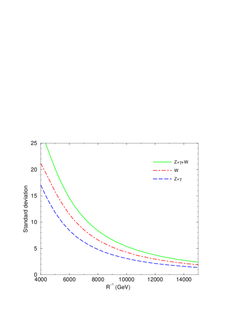
Figure 4: Number of standard deviation in the number of $l^{+}l^{-}$ pairs and $\nu_{l}l$ pairs produced from the expected standard model value due to the presence of one extra-dimension of radius $R$.

In the case of $(l,l,l)$ scenario, looking for an excess of dijet events due to KK excitations of gluons could be the most efficient channel to constrain the size of extra-dimensions. Fig. 5 shows the corresponding expected deviation $\Delta_{T}$ as defined in (62). This analysis uses summation over all jets, top excluded, a rapidity cut, $|\eta|\leq$ 0.5, on both jets and requirement on the invariant mass to be $M_{jj^{\prime}}\geq$ 2 TeV, which reduces the SM background and gives the optimal ratio $S/\sqrt{B}$ expecially for large masses [43].

Figure 5: Number of standard deviation in number of observerd dijets from the expected standard model value, due to the presence of a TeV-scale extra-dimension of compactification radius $R$.

In addition to these virtual effects, the LHC experiments allow the production on-shell of KK excitations. The discovery limits for these KK excitations are given in Table 1. An interesting observation is the case of excitations $\gamma^{(1)}+Z^{(1)}$ where interferences lead to a “deep” just before the resonance as illustrated in Fig. 6

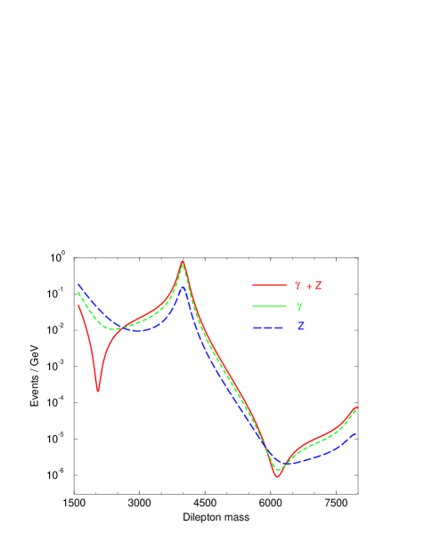
Figure 6: First resonances in the LHC experiment due to a KK excitation of photon and Z for one extra-dimension at 4 TeV. From highest to lowest: excitation of photon+Z, photon and Z boson.

There are some ways to distinguish the corresponding signals from other possible origin of new physics, such as models with new gauge bosons. In the case of observation of resonances, one expects three resonances in the $(l,l,l)$ case and two in the $(t,l,l)$ and $(t,l,t)$ cases, located practically at the same mass value. This property is not shared by most of other new gauge boson models. Moreover, the heights and widths of the resonances are directly related to those of standard model gauge bosons in the corresponding channels. In the case of virtual effects, these are not reproduced by a tail of Bright-Wigner shape and a deep is expected just before the resonance of the photon+$Z$, due to the interference between the two. However, good statistics will be necessary[44].

6.3 High precision data low-energy bounds

Using the lagrangian describing interactions of the standard model states, it is possible to compute all physical observables in term of few input data. Then one can compare the predictions with experimental values.

Following  [47, 48] we will use as input parameters, the Fermi constant $G_{F}=1.166\times 10^{-5}$ GeV^-2, the fine-structure constant $\alpha=1/137.036$ (or $\alpha(M_{Z})=1/128.933$) and the mass of the $Z$ gauge-boson $M_{Z}=91.1871$ GeV. The observables given in Table 3 are then computed with the new lagrangian including the contribution of KK excitations. The effects of the latter will be computed as a leading order expansion in the small parameter

$$X=\sum_{n=1}^{\infty}\frac{2}{n^{2}}\,\frac{m_{Z}^{2}}{M_{c}^{2}}=\frac{\pi^{2}}{3}{(m_{Z}R_{\parallel})}^{2}\,,$$ (73)

as one expects $m_{Z}\ll 1/R_{\parallel}$.

Here we follow  [48] and summarize the bounds in the case where all fermions are localized. Other possibilities have been discussed in  [48]. The results depend on the choice of Higgs fields to be localized or bulk states. In the case where the Higgs scalar is localized, it does not conserve internal momentum and its vacuum expectation value could mix different KK excitations with massless gauge bosons. To include both possibilities of identification of Higgs scalar with localized or bulk states, we consider the Standard model with two Higgs doublets, $H_{i}\ (i=1,2)$, with $v^{2}\equiv\langle H_{1}\rangle^{2}+\langle H_{2}\rangle^{2}$ and $v\simeq 174$ GeV, and introduce the following mixing angles:

$$\tan\beta = \langle H_{2}\rangle/\langle H_{1}\rangle$$ (74)

$$\sin^{2}\alpha = \varepsilon^{H_{2}}\,\sin^{2}\beta+\varepsilon^{H_{1}}\,\cos^{2}\beta$$ (75)

with the operator $\varepsilon$ defined as $\varepsilon^{\phi}=1\ (0)$ for the field $\phi$ localized or not.

The relevant part of the lagrangian is then:

$${\mathcal{L}}={\mathcal{L}}^{neutral}+\sum_{a=1}^{2}{\mathcal{L}}_{a}^{ch}$$ (76)

where the neutral current sector part takes the form:

$${\mathcal{L}}^{neutral} = \frac{1}{2}m_{Z}^{2}Z\cdot Z+\frac{1}{2}\sum_{n=1}^{\infty}M^{2}_{\vec{n}}\,\left[Z^{(n)}\cdot Z^{(n)}+A^{(n)}\cdot A^{(n)}\right]$$ (77)

$$+ \sqrt{2}\sin^{2}{\alpha}m_{Z}^{2}\sum_{n=1}^{\infty}Z\cdot Z^{(n)}$$

$$- \frac{e}{\sin{\theta}\cos{\theta}}\left[Z_{\mu}+\sqrt{2}\sum_{n=1}^{\infty}{Z^{(n)}}_{\mu}\right]\left[\sum_{\psi}\bar{\psi}\,\gamma^{\mu}\left(g_{V}^{\psi}+\gamma_{5}\,g_{A}^{\psi}\right)\psi\,\right]$$

$$- e\left[A_{\mu}+\sqrt{2}\sum_{n=1}^{\infty}A^{(n)}_{\mu}\right]\left[\sum_{\psi}Q_{\psi}\bar{\psi}\,\gamma^{\mu}\psi\,\right]\,,$$

while for the charged currents sector:

$${\mathcal{L}}_{a}^{ch} = \frac{1}{2}m^{2}_{W}W_{a}\cdot W_{a}+\frac{1}{2}\sum_{n=1}^{\infty}\,M^{2}_{\vec{n}}\,W_{a}^{(n)}\cdot W_{a}^{(n)}$$ (78)

$$+ m^{2}_{W}\sqrt{2}\sin^{2}{\alpha}\sum_{n=1}^{\infty}W_{a}\cdot W_{a}^{(n)}$$

$$- g\,\left[{W_{a}}_{\mu}-\,\sqrt{2}\sum_{n=1}^{\infty}{W_{a}^{(n)}}_{\mu}\right]\left[\sum_{\psi}\bar{\psi}_{L}\gamma^{\mu}\frac{\sigma_{a}}{2}\psi_{L}\right]$$

with $m^{2}_{W}=g^{2}v^{2}/2$, $m^{2}_{Z}=(g^{2}+g^{\prime\,2})v^{2}/2$, $\theta$ is the weak mixing angle defined by the usual relation $e=g\,\sin\theta=g^{\prime}\,\cos\theta$ . For energies much below the electroweak scale the gauge bosons can be integrated out leading to effective four-fermion operators:

$${\mathcal{L}}_{low} = -\,\frac{1}{2\left[1-\sin^{4}{\alpha}\,X\right]m_{Z}^{2}}\,\frac{e^{2}}{s^{2}_{\theta}\,c^{2}_{\theta}}\,\left[\left(1-\sin^{2}\alpha\,X\right)^{2}-X\right]{\left[\sum_{\psi}\bar{\psi}\,\gamma^{\mu}\left(g_{V}^{\psi}+\gamma_{5}\,g_{A}^{\psi}\right)\psi\,\right]^{2}}$$

$$- eA^{\mu}\left[\sum_{\psi}Q_{\psi}\bar{\psi}\,\gamma^{\mu}\psi\,\right]$$

$$- X\frac{e^{2}}{2\,\left[1-\sin^{4}\alpha\,X\right]m_{Z}^{2}}\,\left[\sum_{\psi}Q_{\psi}\bar{\psi}\,\gamma_{\mu}\psi\,\right]\left[\sum_{\psi}Q_{\psi}\bar{\psi}\,\gamma^{\mu}\psi\,\right]$$

$$- \frac{g^{2}}{2M_{W}^{2}}\left\{\left[1-\sin^{2}\alpha\,\cos^{2}\theta\,X\right]^{2}+\,\cos^{2}\theta\,X\right\}\left[\sum_{\psi}\bar{\psi}_{L}\gamma_{\mu}\frac{\sigma_{a}}{2}\psi_{L}\right]\left[\sum_{\psi}\bar{\psi}_{L}\gamma^{\mu}\frac{\sigma_{a}}{2}\psi_{L}\right]$$

Using this lagrangian it is possible to extract prediction for the LEP (high-energy) observables:

$${\displaystyle M_{W}^{2}} = \left(M_{W}^{2}\right)^{SM}\left[1-\frac{\sin^{2}{\theta}}{\cos{2\theta}}(\cos{2\alpha}\cos^{2}{\theta}-\sin^{4}{\alpha}\sin^{2}{\theta}+\sin^{4}{\alpha}\cos{2\theta})\,X\right]$$

$${\displaystyle\frac{\Gamma_{\ell\,\ell}}{\Gamma_{\ell\,\ell}^{SM}}} = \left[1-(\cos{2\alpha}\cos^{2}{\theta}-\sin^{4}{\alpha}\sin^{2}{\theta}-2\sin^{2}{\alpha})\,X\right]\,,$$

$${\displaystyle\frac{\Gamma_{had}}{\Gamma_{had}^{SM}}} = \left[1-(\cos{2\alpha}\cos^{2}{\theta}-\sin^{4}{\alpha}\sin^{2}{\theta}-2\sin^{2}{\alpha})\,X\right]\,,$$ (80)

$${\displaystyle\frac{A_{FB}^{\ell}}{A_{FB}^{\ell,\,SM}}} = 1\,,$$

and for the low energy observables:

$$Q_{W}=\left[1-(\cos{2\alpha}\cos^{2}{\theta}-\sin^{4}{\alpha}\sin^{2}{\theta})X\right]\,Q_{W}^{SM}+16\,\delta\,Q_{W}\,,$$ (81)

where

$$\delta Q_{W} = -\frac{1}{4}\,\frac{s^{2}_{\theta}\,c^{2}_{\theta}}{c_{2\theta}}\,Z\,(\cos{2\alpha}\cos^{2}{\theta}-\sin^{4}{\alpha}\sin^{2}{\theta})X$$ (82)

$$+ \,X\,\left\{(2Z+N)\left[g_{A}^{e}g_{V}^{u}-\frac{1}{4}\sin^{2}\alpha\,g_{V}^{u}-\sin^{2}\alpha\,\left(\frac{1}{4}-\frac{2}{3}\sin^{2}{\theta}\right)g_{A}^{e}\right]\right.$$

$$+ \left.(Z+2N)\left[g_{A}^{e}g_{V}^{d}-\frac{1}{4}\sin^{2}\alpha\,g_{V}^{d}-\sin^{2}\alpha\,\left(-\frac{1}{4}+\frac{1}{3}\sin^{2}{\theta}\right)g_{A}^{e}\right]\right\}$$

The experiments are carried with Cesium atoms for which the number of protons and neutrons are $Z=55$ and $N=78$, while $\sum_{q^{\prime}}\left|V_{uq^{\prime}}\right|^{2}=1$ does not receive corrections at the leading order. Performing a $\chi^{2}$ fit, one finds for example that if the Higgs is assumed to be a bulk state ($\alpha=0$) like the gauge bosons, $R^{-1}\mathrel{\lower 2.5pt\vbox{\hbox{$>$}\hbox{$\sim$}}}3.5$ TeV. Inclusion of $Q_{W}$ measurement, which does not give a good agreement with the standard model itself, raises the bound to $R^{-1}\mathrel{\lower 2.5pt\vbox{\hbox{$>$}\hbox{$\sim$}}}3.9$ TeV [48]. Different choices for localization of matter states and Higgs lead to slightly different bounds, lying in the 1 to 5 TeV range, and the analysis can be found in  [48].

6.4 One extra dimension for other cases:

Except for the $(l,l,l)$ scenario, in all other cases there are no excitations of gluons and there no important limits from the dijets channels [43].

The KK excitations $W_{\pm}^{(n)}$, $\gamma^{(n)}$ and $Z^{(n)}$ are present and lead to the same limits in the $(t,l,l)$ case: 6 TeV for discovery and 15 TeV for the exclusion bounds.

In the $(t,l,t)$ case, only the $SU(2)$ factor feels the extra-dimension and the limits are set by KK excitations of $W^{\pm}$ and are again 6 TeV for discovery and 14 TeV for the exclusion bounds.

In the $(t,t,l)$ channel where only $U(1)_{Y}$ feels the extra-dimension the limits are weaker, the exclusion bound is in fact around 8 TeV, as can be seen in Fig. 7.

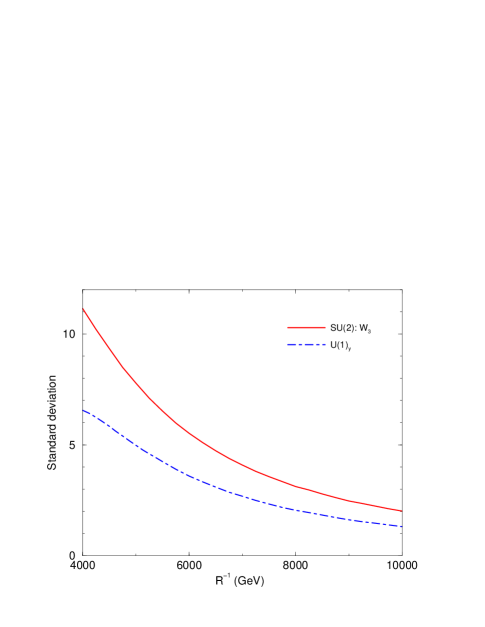
Figure 7: Number of standard deviation in the number of $l^{+}l^{-}$ pairs produced from the expected standard model value due to the presence of one extra-dimension of radius $R$ in the case of $(t,l,t)$ i.e. $W_{3}$ KK excitations and the case of $(t,t,l)$ i.e. $U(1)_{Y}$ boson KK excitations.

In addition to these simple possibilities, brane constructions lead often to cases where part of $U(1)_{Y}$ is $t$ and part is $l$, while $SU(3)$ and $SU(2)$ are either $t$ or $l$. If $SU(3)$ is $l$ then the bounds come from dijets, if instead $SU(3)$ is $t$ and $SU(2)$ is $l$ the limits could come from $W^{\pm}$ while if both are $t$ then it will be difficult to distinguish this case from a generic extra $U(1)^{\prime}$. A good statistics would be needed to see the deviation in the tail of the resonance as being due to effects additional to those of a generic $U(1)^{\prime}$ resonance.

6.5 More than one extra dimensions

The computation of virtual effects of KK excitations involves summing on effects of a priori infinite number of tree-level diagrams as terms of the form:

$$\sum_{|\vec{n}|}\frac{g^{2}{(|\vec{n}|)}}{|\vec{n}|^{2}}$$ (83)

arising from interference between the exchange of the photon and $Z$-boson and their KK excitations, with $g^{2}(|\vec{n}|)$ the KK-mode couplings. In the case of one extra-dimension the sum in (83) converges rapidly and for $RM_{s}\sim{\cal O}(10)$ the result is not sensitive to the value of $M_{s}$. This alowed us to discuss bounds on only one paprameter, the scale of compactification.

In the case of two or more dimensions, Eq. (83) is divergent and needs to be regularized using:

$$g(|\vec{n}|)\sim g\;a_{(|\vec{n}|)}\;e^{\frac{-c|\vec{n}|^{2}}{2R^{2}M_{s}^{2}}}\,,$$ (84)

where $c$ is a constant and $a_{(|\vec{n}|)}$ takes into account the normalization of the gauge kinetic terms, as only the even combination couples to the boundary. For the case of two extra-dimensions [45] $a_{(0,0)}=1$, $a_{(0,p)}=a_{(q,0)}=\sqrt{2}$ and $a_{(q,p)}=2$ with $(p,q)$ positive ($>0$) integers. The result will depend on both the compactification and string scales. Other features are that cross-sections are bigger and resonances are closer. The former property arises because the degeneracy of states within each mass level increases with the number of extra dimensions while the latter property implies that more resonances could be reached by a given hadronic machine.

7 Extra-dimensions transverse to the world brane: KK excitations of gravitons

The localization of (infinitely massive) branes in the $(D-d)$ dimensions breaks translation invariance along these directions. Thus, the corresponding momenta are not conserved: particles, as gravitons, could be absorbed or emitted from the brane into the $(D-d)$ dimensions. Non observation of the effects of such processes allow us to get bounds on the size of these transverse extra dimensions. In order to simplify the analysis, it is usually assumed that among the $D-d$ dimensions $n$ have very large common radius $R_{\perp}\gg M_{s}^{-1}$, while the remaining $D-d-n$ have sizes of the order of the string length.

7.1 Signals from missing energy experiments

During a collision of center of mass energy $\sqrt{s}$, there are $(\sqrt{s}R_{\perp})^{n}$ KK excitations of gravitons with mass $m_{KK\perp}<\sqrt{s}<M_{s}$, which can be emitted. Each of these states looks from the four-dimensional point of view as a massive, quasi-stable, extremely weakly coupled ($s/M^{2}_{pl}$ suppressed) particle that escapes from the detector. The total effect is a missing-energy cross section roughly of order:

$$\frac{(\sqrt{s}R_{\perp})^{n}}{M^{2}_{pl}}\sim\frac{1}{s}{(\frac{\sqrt{s}}{M_{s}})^{n+2}}$$ (85)

For illustration, the simplest process is the gluon annihilation into a graviton which escapes into the extra dimensions. The corresponding cross-section is given by (in the weak coupling limit) [11]:

$$\sigma(E)\sim{E^{n}\over M_{s}^{n+2}}{\Gamma\left(1-2E^{2}/M_{s}^{2}\right)^{2}\over\Gamma\left(1-E^{2}/M_{s}^{2}\right)^{4}}\,,$$ (86)

where $E$ is the center of mass energy and $n$ the number of extra large transverse dimensions. The above expression exhibits 3 kinematic regimes with different behavior. At high energies $E\gg M_{s}$, it falls off exponentially due to the UV softness of strings. At energies of the order of the string scale, it exhibits a sequence of poles at the position of Regge resonances. Finally, at low energies $E\ll M_{s}$, it falls off as a power $\sigma(E)\sim E^{n}/M_{s}^{n+2}$, dictated by the effective higher dimensional gravity which requires the presence of the $(4+n)$-dimensional Newton’s constant $G_{N}^{(4+n)}\sim l_{s}^{n+2}$ from eq.(14).

Explicit computation of these effects leads to the bounds given in table 2 [50]. The results require some remarks:

• The amplitude for emission of each of the KK gravitons is taken to be well approximated by the tree-level coupling of the massless graviton as derived from General Relativity. Eq. 3 suggests that this is likely to be a good approximation for $R_{\perp}M_{s}\gg 1$.

• The cross-section depends on the size $R_{\perp}$ of the transverse dimensions and allows to derive bounds on this physical scale. As it can be seen from Eq. (3), transforming these bounds to limits on $M_{s}$ there is an ambiguity on different factors involved, such as the string coupling. This is sometimes absorbed in the so called “fundamental quantum gravity scale $M_{(4+n)}$”. Generically $M_{(4+n)}$ is bigger than $M_{s}$, and in some cases, as in type II strings or in heterotic strings with small instantons, it can be many orders of magnitude higher than $M_{s}$. It corresponds to the scale where the perturbative expansion of string theory seems to break down [51].

• There is a particular energy and angular distribution of the produced gravitons that arises from the distribution in mass of KK states given in Eq. (1). It might be a smoking gun for the extra-dimensional nature of such observable signal.

• For given value of $M_{s}$, the cross section for graviton emission decreases with the number of large transverse dimensions. The effects are more likely to be observed for the lowest values of $M_{s}$ and $n$.

• Finally, while the obtained bounds for $R_{\perp}^{-1}$ are smaller than those that could be checked in table-top experiments probing macroscopic gravity at small distances (see next subsection), one should keep in mind that larger radii are allowed if one relaxes the assumption of isotropy, by taking for instance two large dimensions with different radii.

In table 2, we have also included astrophysical and cosmological bounds. Astrophysical bounds [54, 52] arise from the requirement that the radiation of gravitons should not carry on too much of the gravitational binding energy released during core collapse of supernovae. In fact, the measurements of Kamiokande and IMB for SN1987A suggest that the main channel is neutrino fluxes.

The best cosmological bound [53] is obtained from requiring that decay of bulk gravitons to photons do not generate a spike in the energy spectrum of the photon background measured by the COMPTEL instrument. Bulk gravitons are expected to be produced just before nucleosynthesis due to thermal radiation from the brane. The limits assume that the temperature was at most 1 MeV as nucleosynthesis begins, and become stronger if the temperature is increased.

7.2 Gravity modification and sub-millimeter forces

Besides the spectacular experimental predictions in particle accelerators, string theories with large volume compactifications and/or low string scale predict also possible modifications of gravitation in the sub-millimeter range, which can be tested in “tabletop” experiments that measure gravity at short distances. There are two categories of such predictions:
(i) Deviations from the Newton’s law $1/r^{2}$ behavior to $1/r^{2+n}$, for $n$ extra large transverse dimensions, which can be observable for $n=2$ dimensions of sub-millimeter size. This case is particularly attractive on theoretical grounds because of the logarithmic sensitivity of Standard Model couplings on the size of transverse space, but also for phenomenological reasons since the effects in particle colliders are maximally enhanced [50]. Notice also the coincidence of this scale with the possible value of the cosmological constant in the universe that recent observations seem to support.
(ii) New scalar forces in the sub-millimeter range, motivated by the problem of supersymmetry breaking discussed in section 4.3, and mediated by light scalar fields $\varphi$ with masses [55, 49, 11, 35]:

$$m_{\varphi}\simeq{m_{susy}^{2}\over M_{P}}\simeq 10^{-4}-10^{-2}\ {\rm eV}\,,$$ (87)

for a supersymmetry breaking scale $m_{susy}\simeq 1-10$ TeV. These correspond to Compton wavelengths in the range of 1 mm to 10 $\mu$m. $m_{susy}$ can be either the KK scale $1/R$ if supersymmetry is broken by compactification [49], or the string scale if it is broken “maximally” on our world-brane [11, 35]. A model independent scalar force is mediated by the radius modulus (in Planck units)

$$\varphi\equiv\ln R\,,$$ (88)

with $R$ the radius of the longitudinal or transverse dimension(s), respectively. In the former case, the result (87) follows from the behavior of the vacuum energy density $\Lambda\sim 1/R^{4}$ for large $R$ (up to logarithmic corrections). In the latter case, supersymmetry is broken primarily on the brane only, and thus its transmission to the bulk is gravitationally suppressed, leading to masses (87).

The coupling of these light scalars to nuclei can be computed since it arises dominantly through the radius dependence of $\Lambda_{\rm QCD}$, or equivalently of the QCD gauge coupling. More precisely, the coupling $\alpha_{\phi}$ of the radius modulus (88) relative to gravity is [49]:

$$\alpha_{\varphi}={1\over m_{N}}{\partial m_{N}\over\partial\varphi}={\partial\ln\Lambda_{\rm QCD}\over\partial\ln R}=-{2\pi\over b_{\rm QCD}}{\partial\over\partial\ln R}\alpha_{\rm QCD}\,,$$ (89)

with $m_{N}$ the nucleon mass and $b_{\rm QCD}$ the one-loop QCD beta-function coefficient. In the case where supersymmetry is broken primordially on our world-brane at the string scale while it is almost unbroken the bulk, the force (3) is again comparable to gravity in theories with logarithmic sensitivity on the size of transverse space, i.e. when there is effective propagation of gravity in $d_{\perp}=2$ transverse dimensions. The resulting forces can therefore be within reach of upcoming experiments [15].

In principle there can be other light moduli which couple with even larger strengths. For example the dilaton $\phi$, whose VEV determines the (logarithm of the) string coupling constant, if it does not acquire large mass from some dynamical supersymmetric mechanism, can lead to a force of strength 2000 times bigger than gravity [56].

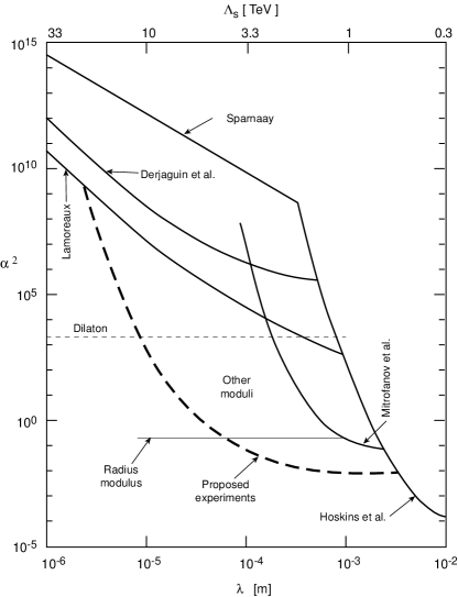
Figure 8: Strength of the modulus force relative to gravity ($\alpha^{2}$) versus its Compton wavelength ($\lambda$).

In fig. 8 we depict the actual information from previous, present and upcoming experiments [15]. The vertical axis is the strength, $\alpha^{2}$, of the force relative to gravity; the horizontal axis is the Compton wavelength of the exchanged particle; the upper scale shows the corresponding value of the supersymmetry breaking scale (large radius or string scale) in TeV. The solid lines indicate the present limits from the experiments indicated. The excluded regions lie above these solid lines. Measuring gravitational strength forces at such short distances is quite challenging. The most important background is the Van der Walls force which becomes equal to the gravitational force between two atoms when they are about 100 microns apart. Since the Van der Walls force falls off as the 7th power of the distance, it rapidly becomes negligible compared to gravity at distances exceeding 100 $\mu$m. The dashed thick line gives the expected sensitivity of the present and upcoming experiments, which will improve the actual limits by roughly two orders of magnitude and –at the very least– they will, for the first time, measure gravity to a precision of 1% at distances of $\sim$ 100 $\mu$m.

8 Dimension-eight operators and limits on the string scale

At low energies, the interaction of light (string) states is described by an effective field theory. Non-renormalizable dimension-six operators are due to the exchange of KK excitations of gauge bosons between localized states. If these are absent, then there are deviations to the standard model expectations from dimension-eight operators. There are two generic sources for such operators: exchange of virtual KK excitations of bulk fields (gravitons,…) and form factors due to the extended nature of strings.

The exchange of virtual KK excitations of bulk gravitons is described in the effective field theory by an amplitude involving the sum $\frac{1}{M_{p}^{2}}\sum_{n}\frac{1}{s-\frac{{\vec{n}}^{2}}{R_{\perp}^{2}}}$. For $n>1$, this sum diverges and one cannot compute it in field theory but only in a fundamental (string) theory. In analogy with the case of exchange of gauge bosons, one expects the string scale to act as a cut-off with the result:

$$Ag_{s}^{2}\frac{T_{\mu\nu}T^{\mu\nu}-\frac{1}{1+d_{\perp}}T_{\mu}^{\mu}T_{\nu}^{\nu}}{M_{s}^{4}}\,.$$ (90)

The approximation $A=\log{\frac{M_{s}^{2}}{s}}$ for $d_{\perp}=2$ and $A=\frac{2}{d_{\perp}-2}$ for $d_{\perp}>2$ is usually used for quantitative discussions. There are some reasons which might invalidate this approximation in general. In fact, the result is very much model dependent: in type I string models it reflects the ultraviolet behavior of open string one-loop diagrams which are model (compactification) dependent.

In order to understand better this issue, it is important to remind that in type I string models, gravitons and other bulk particles correspond to excitations of closed strings. Their tree-level exchange is described by a cylinder joining the initial $|Bin>$ and final $|Bout>$ closed strings lying on the brane. This cylinder can be be seen on the other hand as an open string with one of its end-points describing the closed (loop) string $|Bin>$, while the other end draws $|Bout>$. In other words, the cylinder can be seen as an annulus which is a one-loop diagram of open strings with boundaries $|Bin>$ and $|Bout>$. Note that usually the theory requires the presence of other weakly interacting closed strings besides gravitons.

More important is that when the gauge degrees of freedom arise from Dirichelet branes, it is expected that the dominant source of dimension-eight operators is not the exchange of KK states but instead the effects of massive open string oscillators [43, 57]. These give rise to contributions to tree-level scatterings that behave as $g_{s}s/M_{s}^{4}$. Thus, they are enhanced by a string-loop factor $g_{s}^{-1}$ compared to the field theory estimate based on KK graviton exchanges. Although the precise value of $g_{s}$ requires a detail analysis of threshold corrections, a rough estimate can be obtained by taking $g_{s}\simeq\alpha\sim 1/25$, implying an enhancement by one order of magnitude, and in any case a loop-factor as consequence of perturbation theory.

What is the simplest thing one could do in practice?. There are some processes for which there is only one allowed dimension-eight operator; an example is $f{\bar{f}}\rightarrow\gamma\gamma$. The coefficient of this operator can then be computed in terms of $g_{s}$ and $M_{s}$. As a result, in the only framework where computation of such operators is possible to carry out, one cannot rely on the effects of exchange of KK graviton excitations in order to derive bounds on extra-dimensions or the string scale. Instead, one can use the dimension-eight operator arising from stringy form-factors.

Under the assumption that the electrons arise as open strings on a $D3$-brane, and not as living on the intersections of different kind of branes, an estimate at the lowest order approximation of string form factor in type I was used in [57]. For instance for $e^{+}e^{-}\to\gamma\gamma$ one has:

$${d\sigma\over d\cos\theta}={d\sigma\over d\cos\theta}\biggr{|}_{SM}\cdot\left[1+{\pi^{2}\over 12}{ut\over M_{S}^{4}}+\cdots\right]$$ (91)

while for Bhabha scattering, it was suggested that

$${d\sigma\over d\cos\theta}(e^{-}e^{+}\to e^{-}e^{+})={d\sigma\over d\cos\theta}\biggr{|}_{SM}\cdot\left|{\Gamma(1-\frac{s}{M_{s}^{2}})\Gamma(1-\frac{t}{M_{s}^{2}})\over\Gamma(1-\frac{s}{M_{s}^{2}}-\frac{t}{M_{s}^{2}})}\right|^{2}\ ,$$ (92)

where $s$ and $t$ are the Mandelstam kinematic variables. Using these estimates, present LEP data lead to limits on the string scale $M_{s}\mathrel{\lower 2.5pt\vbox{\hbox{$>$}\hbox{$\sim$}}}1$ TeV. This translates into a stronger bound on the size of transverse dimension than those obtained from missing energy experiments in the cases $d_{\perp}>2$.

9 Conclusions

The theoretical possibility of a string scale lying at energies much lower than the four-dimensional Planck scale opens up a new insight on problems of physics beyond the standard model. Moreover it calls for two urgent investigations: one is to derive limits on the possible scales of new physics associated with compactification and string scales from present experiments, and the second is to understand possible signatures of this new physics at future experiments.

We have stressed that addressing these issues requires a well defined theoretical framework, for instance the choice of a vacuum of string theory. One of the issues which illustrates this necessity is for instance four-fermion operators which are due to exchanges of virtual KK excitation of the graviton. In addition to providing new bounds on the size of transverse dimensions to the brane, these effects were expected to lead to observable deviations in cross-sections with an angular dependence typical of the exchange of spin-two states. This would provide us with a spectacular signature of quantum gravitational effects. However such effects can only be analysed in a consistent theory of quantum gravity: string theory. Unfortunately, carrying such an analysis shows that in fact these higher dimensional operators are dominated by string form factors due to excitation of oscillation modes of the strings and thus one does not expect to measure effects due to virtual exchange of gravitons.

Understanding features of string vacua and building realistic string models will certainly shed some light on some other issues which were not covered by this review. We can cite for instance:

• Lowering the string scale, one increases the strength of higher (non-renormalizable) operators leading to the possibility of inducing exotic processes at experimentally excluded rates, as for proton decay and flavour changing processes. Although an explicit string realization of the scenario is necessary in order to have a satisfactory solution, at the effective field theory level many discrete or global symmetries can be displayed that forbid these operators.

• As we have stressed in section 3, string vacua with arbitrarely low string scale is a consequence of the existence of mechanisms ($D$-branes) for localizing gauge degrees of freedom. Is it also possible to localize gravitons? Starting with 5-dimensional gravity, it was shown in [58] that there exist metrics, a slice of Anti-de-Sitter space where gravity is localized. The possible application for phenomenological purposes of such a scenario necessites then understanding the origin of the other (gauge and matter) states. For instance, if these are localized on a brane at the boundary of this space, then what is the nature of this brane and of the theory leaving on its world-volume? and what kind of modifications (or extensions if any) of the original proposal of [58] are needed in order to have a consistent embedding in string theory? These issues are related to each other and they constitute a intensive subject of research at the present time.

References

Table 1: Limits on $R^{-1}_{\parallel}$ in TeV at present and future colliders. The luminosity is given in fb^-1.

Collider	Luminosity	Gluons	$W^{\pm}$	$\gamma+Z$
Discovery of Resonances
LHC	100	5	6	6
Observation of Deviation
LEP 200	$4\times 0.2$	-	-	1.9
TevatronI	$0.11$	-	-	0.9
TevatronII	2	-	-	$1.2$
TevatronII	20	4	-	1.3
LHC	10	15	8.2	6.7
LHC	100	20	14	12
NLC500	75	-	-	8
NLC1000	200	-	-	13

Table 2: Limits on $R_{\perp}$ in mm from missing-energy processes.

Experiment	$R_{\perp}(n=2)$	$R_{\perp}(n=4)$	$R_{\perp}(n=6)$
Collider bounds
LEP 2	$4.8\times 10^{-1}$	$1.9\times 10^{-8}$	$6.8\times 10^{-11}$
Tevatron	$5.5\times 10^{-1}$	$1.4\times 10^{-8}$	$4.1\times 10^{-11}$
LHC	$4.5\times 10^{-3}$	$5.6\times 10^{-10}$	$2.7\times 10^{-12}$
NLC	$1.2\times 10^{-2}$	$1.2\times 10^{-9}$	$6.5\times 10^{-12}$
Present non-collider bounds
SN1987A	$3\times 10^{-4}$	$1\times 10^{-8}$	$6\times 10^{-10}$
COMPTEL	$5\times 10^{-5}$	-	-

Table 3: Set of physical observables. The Standard Model predictions are computed for a Higgs mass $M_{H}=M_{Z}$ ($M_{H}=300$ GeV) and a top-quark mass $m_{t}=173\pm 4$ GeV.

Observable	Experimental value	Standard Model prediction
$M_{W}$ (GeV)	80.394$\pm$0.042	80.377$\pm$0.023 ($-$0.036)
$\Gamma_{\ell\ell}$ (MeV)	83.958$\pm$0.089	84.00$\pm$0.03 ($-$0.04)
$\Gamma_{had}$ (GeV)	1.7439$\pm$0.0020	1.7433$\pm$0.0016 ($-$0.0005)
$A_{FB}^{\ell}$	0.01701$\pm$0.00095	0.0162$\pm$0.0003 ($-0.0004$)
$Q_{W}$	$-$72.06$\pm$0.46	$-$73.12$\pm$0.06 ($+$0.01)
$\sum_{i=1}^{3}\left|V_{1i}\right|^{2}$	0.9969$\pm$0.0022	1 (unitarity)

References

- [1] I. Antoniadis, C. Bachas, D. Lewellen and T. Tomaras, Phys. Lett. B 207, 441 (1988).
- [2] C. Kounnas and M. Porrati, Nucl. Phys. B 310, 355 (1988); S. Ferrara, C. Kounnas, M. Porrati and F. Zwirner, Nucl. Phys. B 318, 75 (1989).
- [3] I. Antoniadis, Phys. Lett. B 246, 377 (1990).
- [4] T. Taylor and G. Veneziano, Phys. Lett. B 212, 147 (1988).
- [5] I. Antoniadis and B. Pioline, Nucl. Phys. B 550, 41 (1999), hep-th/9902055.
- [6] E. Witten, Proceedings of Strings 95, hep-th/9507121; A. Strominger, Phys. Lett. B 383, 44 (1996);B475, 94 (1996).
- [7] N. Seiberg, Phys. Lett. B 390, 169 (1997).
- [8] E. Witten, Nucl. Phys. B 471, 135 (1996).
- [9] J.D. Lykken, Phys. Rev. D 54, 3693 (1996), G. Shiu and S.-H.H. Tye, Phys. Rev. D 58, 106007 (1998); Z. Kakushadze and S.-H.H. Tye, Nucl. Phys. B 548, 180 (1999).
- [10] N. Arkani-Hamed, S. Dimopoulos and G. Dvali, Phys. Lett. B 429, 263 (1998).
- [11] I. Antoniadis, N. Arkani-Hamed, S. Dimopoulos and G. Dvali, Phys. Lett. B 436, 263 (1998).
- [12] I. Antoniadis, C. Bachas, Phys. Lett. B 450, 99 (83).
- [13] K. Benakli, Phys. Rev. D 60, 104002 (1999).
- [14] C.P. Burgess, L.E. Ibáñez, F. Quevedo, Phys. Lett. B 429, 257 (1999).
- [15] See for instance: J.C. Long, H.W. Chan and J.C. Price, Nucl. Phys. B 539, 23 (1999).
- [16] P. Hořava and E. Witten, Nucl. Phys. B 460, 506 (1996).
- [17] E. Witten, Nucl. Phys. B 471, 135 (1996);
- [18] K. Benakli, Phys. Lett. B 447, 51 (1999); S. Stieberger, Nucl. Phys. B 541, 109 (1999); Z. Lalak, S. Pokorski and S. Thomas, Nucl. Phys. B 549, 63 (1999); D.G. Cerdeño and C. Muñoz, Phys. Rev. D 61, 016001 (2000).
- [19] E. Witten, Nucl. Phys. B 460, 541 (1996).
- [20] K. Benakli and Y. Oz, Phys. Lett. B 472, 83 (2000).
- [21] E. Caceres, V. S. Kaplunovsky and I. M. Mandelberg, Nucl.Phys.B493 73.
- [22] P. S. Aspinwall and D. R. Morrison, Nucl. Phys. B 503, 533 (1997).
- [23] J. D. Blum and K. Intriligator, hep-th/9705044.
- [24] K. Intriligator, hep-th/9708117.
- [25] N. Seiberg and E. Witten, Nucl.Phys. B471, 121 (1996).
- [26] O. Ganor and A. Hanany, Nucl.Phys. B474, 122 (1996) .
- [27] I. Antoniadis and M. Quirós, Phys. Lett. B 392, 61 (1997).
- [28] C.M. Hull and P.K. Townsend, Nucl. Phys. B 438, 109 (1995) and Nucl. Phys. B 451, 525 (1995); E. Witten, Nucl. Phys. B 443, 85 (1995).
- [29] K.R. Dienes, E. Dudas and T. Gherghetta, Phys. Lett. B 436, 55 (1998); Nucl. Phys. B 537, 47 (1999).
- [30] D. Ghilencea and G.G. Ross, Phys. Lett. B 442, 165 (1998); Z. Kakushadze, Nucl. Phys. B 548, 205 (1999); A. Delgado and M. Quirós, Nucl. Phys. B 559, 235 (1999); P. Frampton and A. Rasin, Phys. Lett. B 460, 313 (1999); A. Pérez-Lorenzana and R.N. Mohapatra, Nucl. Phys. B 559, 255 (1999); Z. Kakushadze and T.R. Taylor, Nucl. Phys. B 562, 78 (1999).
- [31] C. Bachas, JHEP 9811, 23 (1998).
- [32] N. Arkani-Hamed, S. Dimopoulos and J. March-Russell, hep-th/9908146.
- [33] I. Antoniadis, C. Bachas and E. Dudas, Nucl. Phys. B 560, 93 (1999).
- [34] S. Kachru and E. Silverstein, JHEP 11, 1 (1998), hep-th/9810129; J. Harvey, Phys. Rev. D 59, 26002 (1999); R. Blumenhagen and L. Görlich, hep-th/9812158; C. Angelantonj, I. Antoniadis and K. Foerger, Nucl. Phys. B 555, 116 (1999), hep-th/9904092.
- [35] I. Antoniadis, E. Dudas and A. Sagnotti, hep-th/9908023; G. Aldazabal and A.M. Uranga, hep-th/9908072.
- [36] C. Bachas, hep-th/9503030; J.G. Russo and A.A. Tseytlin, Nucl. Phys. B 461, 131 (1996).
- [37] I. Antoniadis, E. Dudas and A. Sagnotti, Nucl. Phys. B 544, 469 (1999); I. Antoniadis, G. D’Appollonio, E. Dudas and A. Sagnotti, Nucl. Phys. B 553, 133 (1999) and hep-th/9907184.
- [38] B. Grzadkowski and J.F. Gunion, Phys. Lett. B 473, 50 (2000).
- [39] I. Antoniadis, K. Benakli and M. Quirós, hep-ph/0004091.
- [40] I. Antoniadis, S. Dimopoulos, A. Pomarol and M. Quirós, Nucl. Phys. B 544, 503 (1999); A. Delgado, A. Pomarol and M. Quirós, Phys. Rev. D 60, 095008 (1999).
- [41] J.A. Casas, J.R. Espinosa, M. Quirós and A. Riotto, Nucl. Phys. B 436, 3 (1995); M. Carena, J.R. Espinosa, M. Quirós and C.E.M. Wagner, Phys. Lett. B 355, 209 (1995); M. Carena, M. Quirós and C.E.M. Wagner, Nucl. Phys. B 461, 407 (1996); H.E. Haber, R. Hempfling and A.H. Hoang, Z. Phys. C 75, 539 (1997); M. Carena, H.E. Haber, S. Heinemeyer, W. Hollik, C.E.M. Wagner and G. Weiglein, hep-ph/0001002; J.R. Espinosa and R.-J. Zhang, JHEP 3, 26 (2000).
- [42] I. Antoniadis, C. Muñoz and M. Quirós, Nucl. Phys. B 397, 515 (1993); A. Pomarol and M. Quirós, Phys. Lett. B 438, 225 (1998); I. Antoniadis, S. Dimopoulos, A. Pomarol and M. Quirós, Nucl. Phys. B 544, 503 (1999); A. Delgado, A. Pomarol and M. Quirós, Phys. Rev. D 60, 095008 (1999).
- [43] E. Accomando, I. Antoniadis and K. Benakli, Nucl. Phys. B 579, 3 (2000).
- [44] I. Antoniadis and K. Benakli, Phys. Lett. B 326, 69 (1994), I. Antoniadis, K. Benakli and M. Quirós, Phys. Lett. B 331, 313 (1994); P. Nath, Y. Yamada and M. Yamaguchi, Phys. Lett. B 466, 100 (1999) T.G. Rizzo and J.D. Wells, Phys. Rev. D 61, 016007 (2000); A. De Rujula, A. Donini, M.B. Gavela and S. Rigolin, Phys. Lett. B 482, 195 (2000).
- [45] I. Antoniadis, K. Benakli and M. Quirós, Phys. Lett. B 460, 176 (1999).
- [46] A. Djouadi, A. Leike, T. Riemann, D. Schaile and C. Verzegnassi, Z. Phys. C56 (1992) 289.
- [47] P. Nath and M. Yamaguchi, Phys. Rev. D 60, 116004 (1999); Phys. Rev. D 60, 116006 (1999); M. Masip and A. Pomarol, Phys. Rev. D 60, 096005 (1999); W.J. Marciano, Phys. Rev. D 60, 093006 (1999); A. Strumia, Phys. Lett. B 466, 107 (1999); R. Casalbuoni, S. De Curtis, D. Dominici and R. Gatto, Phys. Lett. B 462, 48 (1999); C.D. Carone, Phys. Rev. D 61, 015008 (2000).
- [48] A. Delgado, A. Pomarol and M. Quirós, JHEP 1, 30 (2000).
- [49] I. Antoniadis, S. Dimopoulos and G. Dvali, Nucl. Phys. B 516, 70 (1998).
- [50] G.F. Giudice, R. Rattazzi and J.D. Wells, Nucl. Phys. B 544, 3 (1999); E.A. Mirabelli, M. Perelstein and M.E. Peskin, Phys. Rev. Lett. 82, 2236 (1999); T. Han, J. D. Lykken and R. Zhang, Phys. Rev. D59, 105006 (1999); K. Cheung and W.-Y. Keung, Phys. Rev. D60, 112003 (1999); S. Cullen and M. Perelstein, Phys. Rev. Lett. 83 (1999) 268; C. Balázs et al., Phys. Rev. Lett. 83 (1999) 2112; L3 Collaboration (M. Acciarri et al.), Phys. Lett. B464, 135 (1999), Phys. Lett. B470, 281 (1999); J.L. Hewett, Phys. Rev. Lett. 82, 4765 (1999); D. Atwood, C.P. Burgess, E. Filotas, F. Leblond, D. London and I. Maksymyk, hep-ph/0007178. For a recent analysis, see [57] and references therein.
- [51] G. Veneziano, Nuovo Cimento 57, 190 (1968); D. J. Gross and P. F. Mende, Phys. Lett. B 197, 129 (1987); Nucl. Phys. B 303, 407 (1988); D. J. Gross and J.L. Manes, Nucl. Phys. B 326, 73 (1989); S.H. Shenker, hep-th/9509132.
- [52] S. Cullen and M. Perelstein, Phys. Rev. Lett. 83, 268 (1999); V. Barger, T. Han, C. Kao and R.J. Zhang, Phys. Lett. B 461, 34 (1999).
- [53] K. Benakli and S. Davidson, Phys. Rev. D 60, 025004 (1999); L.J. Hall and D. Smith, Phys. Rev. D 60, 085008 (1999).
- [54] N. Arkani-Hamed, S. Dimopoulos and G. Dvali, Phys. Rev. D 59, 086004 (1999).
- [55] S. Ferrara, C. Kounnas and F. Zwirner, Nucl. Phys. B 429, 589 (1994).
- [56] T.R. Taylor and G. Veneziano, Phys. Lett. B 213, 450 (1988).
- [57] S. Cullen, M. Perelstein and M.E. Peskin, hep-ph/0001166; D. Bourilkov, hep-ph/0002172; L3 Collaboration (M. Acciarri et al.), hep-ex/0005028.
- [58] L. Randall, R. Sundrum, Phys. Rev. Lett. 83, 4690 (1999)