LUMINOSITY OF ASYMMETRIC e+e- COLLIDER WITH COUPLING LATTICES

Abstract

A formula of luminosity of asymmetric e+e- collider with coupled lattices is derived explicitly. The calculation shows how the tilted angle and aspect ratio of the beams affect the luminosity. Knowing the result of the calculation, we measure the tilted angle of the luminous region of the collision for PEP-II using two dimensional transverse scan of the luminosity. The method could be applied to correct the coupling at the collision point.

1 INTRODUCTION

The luminosity of colliding storage rings is one of the most important criteria of performance. In order to achieve high luminosity, the colliding beams need to be aligned precisely at the collision point in all three dimensions. For a symmetric collider, the alignment of the electron and positron beams is ensured automatically by the symmetries of charge conjugation and time-reversal. Since an asymmetric collider consists of two different storage rings, precise alignment of the two beams at the collision can only be achieved through tuning of the two rings.

In this paper, our goal is to show some effects on the luminosity when the two beams are not aligned well in transverse planes due to the coupling.

2 LINEAR COUPLING

It was shown by Edwards and Teng[1] that a two-dimensional coupled linear motion in a periodic and symplectic system can be parameterized with ten independent parameters as a block diagonalization of a one-turn matrix

$$M=A\cdot R\cdot A^{-1}$$ (1)

where $R$ is the rotation matrix and $A$ defines the symplectic transformation from the normalized coordinates to the physical coordinates. These matrices can be further decomposed into

$$R=\left(\begin{array}[]{clcr}r_{1}&0\\ 0&r_{2}\end{array}\right)$$ (2)

and

$$A=\left(\begin{array}[]{clcr}I\cos\phi&{\bar{w}}\sin\phi\\ -w\sin\phi&I\cos\phi\end{array}\right)\left(\begin{array}[]{clcr}s_{1}&0\\ 0&s_{2}\end{array}\right)$$ (3)

where $I$ is 2$\times$2 identity matrix and $s_{1},s_{2},w$ are 2$\times$2 symplectic matrices with a determinant of unity. The angle $\phi$ is called coupling angle. Here we denote the bar as two-dimensional symplectic conjugate

$${\bar{w}}=-J\cdot w^{T}\cdot J$$ (4)

where $J$ is 2$\times$2 unit symplectic matrix

$$J=\left(\begin{array}[]{clcr}0&1\\ -1&0\end{array}\right).$$ (5)

Recently, it is pointed out by Sagan and Rubin[2] that there exists another solution of parameterization

$$A=\left(\begin{array}[]{clcr}I\cosh\phi&{\bar{w}}\sinh\phi\\ -w\sinh\phi&I\cosh\phi\end{array}\right)\left(\begin{array}[]{clcr}s_{1}&0\\ 0&s_{2}\end{array}\right)$$ (6)

where $\det w=-1$.

In the case of a strongly coupled lattice, for example, the interaction region of the Low Energy Ring(LER) of PEP-II, both solutions are needed for a complete parameterization of the region.

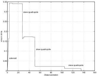
Figure 1: Coupling angle in a half of the interaction region of the LER

Here we choose $\phi$ as a parameter of linear coupling because it has two very important properties: System is decoupled when $\phi=0$ and $\phi$ can be changed only by a skew quadrupole or solenoid as shown in Fig. 1 from which the locations of the skew quadrupoles and solenoid are clearly seen.

3 BEAM PROFILE

In the normalized coordinate, the sigma matrix can be written as

$$\epsilon=\left(\begin{array}[]{clcr}I\epsilon_{1}&0\\ 0&I\epsilon_{2}\end{array}\right)$$ (7)

where $\epsilon_{1}$ and $\epsilon_{2}$ are the equilibrium emittances in the eigen planes ignoring the off-diagonal terms at the order of the damping increment per turn. The sigma matrix in the physical coordinate is obtained with the transformation

$$\Sigma=A\cdot\epsilon\cdot A^{T}.$$ (8)

The corresponding equilibrium Gaussian distribution is

$$\rho(x,P_{x},y,P_{y})={1\over 2\pi{(\det\Sigma)}^{1\over 2}}\exp(-{1\over 2}Z^{T}\cdot\Sigma^{-1}\cdot Z)$$ (9)

where $Z$ is the vector of canonical coordinates. The beam profile in the configuration $x$ and $y$ is derived by integrating the canonical momentum $P_{x}$ and $P_{y}$

$$\rho(x,y)=\int_{-\infty}^{\infty}\int_{-\infty}^{\infty}dP_{x}dP_{y}\rho(x,P_{X},y,P_{y}).$$ (10)

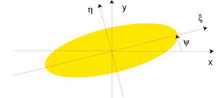
Figure 2: Beam profile

The result of the integration is

$$\rho(x,y)={{(\det K)}^{1\over 2}\over 2\pi}\exp(-{1\over 2}z^{T}\cdot K\cdot z)$$ (11)

where $z$ is the vector of configuration coordinates namely

$$z=\left(\begin{array}[]{cc}x\\ y\end{array}\right)$$ (12)

and $K$ is the inverse of the sigma matrix

$$K={1\over(\sigma_{xx}\sigma_{yy}-\sigma_{xy}\sigma_{yx})}\left(\begin{array}[]{clcr}\sigma_{yy}&-\sigma_{xy}\\ -\sigma_{yx}&\sigma_{xx}\end{array}\right).$$ (13)

Moreover, the symmetric matrix $K$ can be diagonalized by a rotation transformation as shown in Fig. 2

$$\left(\begin{array}[]{cc}\xi\\ \eta\end{array}\right)=\left(\begin{array}[]{clcr}\cos\psi&\sin\psi\\ -\sin\psi&\cos\psi\end{array}\right)\left(\begin{array}[]{cc}x\\ y\end{array}\right),$$ (14)

where $\psi$ is the tilted angle of the beam. The parameters that describe the beam in two coordinate systems relate with each other as following

$$K_{xx} = ({\cos^{2}\psi\over\sigma_{\xi}^{2}}+{\sin^{2}\psi\over\sigma_{\eta}^{2}})$$

$$K_{xy} = ({1\over\sigma_{\xi}^{2}}-{1\over\sigma_{\eta}^{2}})\sin\psi\cos\psi$$

$$K_{yy} = ({\sin^{2}\psi\over\sigma_{\xi}^{2}}+{\cos^{2}\psi\over\sigma_{\eta}^{2}})$$ (15)

and

$$\tan 2\psi = {2K_{xy}\over K_{xx}-K_{yy}}$$

$${1\over\sigma_{\xi}^{2}} = {1\over 2}[(K_{xx}+K_{yy})+{K_{xx}-K_{yy}\over\cos 2\psi}]$$

$${1\over\sigma_{\eta}^{2}} = {1\over 2}[(K_{xx}+K_{yy})-{K_{xx}-K_{yy}\over\cos 2\psi}]$$ (16)

where $K_{xx},K_{xy},K_{yy}$ are the elements of $K$ and $\sigma_{\xi}$ and $\sigma_{\eta}$ are the beam size along the long axis $\xi$ and short axis $\eta$ of the ellipse respectively.

4 LUMINOSITY

For simplicity, we ignore the effect of a finite bunch length. Given the two beam profiles, $\rho_{1}$ and $\rho_{2}$, the luminosity can be written as

$$L=n_{b}f_{0}N_{1}N_{2}\int_{-\infty}^{\infty}\int_{-\infty}^{\infty}\rho_{1}(x,y)\rho_{2}(x,y)dxdy$$ (17)

where $n_{b}$ is the number of the colliding bunches, $f_{0}$ is the revolution frequency, and $N_{1},N_{2}$ are the number of charges in each position and electron bunch respectively.

At a low beam current, the beam distribution is nearly Gaussian. Using Gaussian as an approximation, we can evaluate the overlapping integral

$$L_{2D} = \int_{-\infty}^{\infty}\int_{-\infty}^{\infty}\rho_{1}(x,y)\rho_{2}(x,y)dxdy$$ (18)

$$= {\sqrt{\det K_{1}}\sqrt{\det K_{2}}\over 2\pi\sqrt{\det(K_{1}+K_{2})}}.$$

In order to analyze the result of the calculation, we rewrite the integral in terms of the geometrical parameters, $\sigma_{\xi}$, $\sigma_{\eta}$, and $\psi$ by substituting Eq. 15 into Eq. 18

$$L_{2D}=L_{0}{1\over\sqrt{1+e_{12}\sin^{2}(\psi_{2}-\psi_{1})}}$$ (19)

where

$$L_{0}={1\over 2\pi\sqrt{\sigma_{\xi 1}^{2}+\sigma_{\xi 2}^{2}}\sqrt{\sigma_{\eta 1}^{2}+\sigma_{\eta 2}^{2}}}$$ (20)

and

$$e_{12}={(\sigma_{\xi 1}^{2}-\sigma_{\eta 1}^{2})(\sigma_{\xi 2}^{2}-\sigma_{\eta 2}^{2})\over(\sigma_{\xi 1}^{2}+\sigma_{\xi 2}^{2})(\sigma_{\eta 1}^{2}+\sigma_{\eta 2}^{2})}.$$ (21)

Clearly, the luminosity is at its maximum when $\psi_{2}=\psi_{1}$ which is always the case in a symmetric collider due the symmetries. When two flat beams have identical size, we have

$$e_{12}\approx{\sigma_{\xi}^{2}\over 4\sigma_{\eta}^{2}}.$$ (22)

It is easy to see that the reduction of the luminosity due to the difference of the two tilted angles are much enhanced by the aspect ratio $\sigma_{\xi}$/$\sigma_{\eta}$ of the beams.

5 MEASUREMENT

The luminosity depends upon all six geometrical parameters $\sigma_{\xi 1},\sigma_{\xi 2},\sigma_{\eta 1},\sigma_{\eta 2},\psi_{1}$, and $\psi_{2}$ which describe the size and orientation of the beams. It is impossible to extract these parameters directly from the luminosity alone. By transversely scanning the beam crossing the other one, we could extract more constraints among them.

Let’s calculate the overlapping integral with an offset of centroid of a beam

$$L_{2D}(x_{0},y_{0})=\int_{-\infty}^{\infty}\int_{-\infty}^{\infty}\rho_{1}(x-x_{0},y-y_{0})\rho_{2}(x,y)dxdy.$$ (23)

After a lengthy but straightforward algebra, we obtain

$$L_{2D}(x_{0},y_{0})=L_{2D}\exp(-{1\over 2}z_{0}^{T}\cdot M\cdot z_{0}).$$ (24)

The result agrees with Eq. 19 when $x_{0}=y_{0}=0$. $M$ is a 2$\times$2 symmetric matrix that has the following elements

$$M_{xx}={1\over D}(a_{1}K_{1xx}+a_{2}K_{2xx})$$

$$M_{xy}={1\over D}(a_{1}K_{1xy}+a_{2}K_{2xy})$$

$$M_{yy}={1\over D}(a_{1}K_{1yy}+a_{2}K_{2yy})$$ (25)

where $a=\sigma_{\xi}^{2}\sigma_{\eta}^{2}$ and

$$D=(\sigma_{\xi 1}^{2}+\sigma_{\xi 2}^{2})(\sigma_{\eta 1}^{2}+\sigma_{\eta 2}^{2})[1+e_{12}\sin^{2}(\psi_{2}-\psi_{1})].$$ (26)

Please note that $L_{2D}(x_{0},y_{0})$ is again Gaussian and is normalized to unity

$$\int_{-\infty}^{\infty}\int_{-\infty}^{\infty}L_{2D}(x_{0},y_{0})dx_{0}dy_{0}=1.$$ (27)

Thus, similar to the treatment of the single beam profile, we can diagonalize $M$ with a rotation $\Psi$

$$\tan 2\Psi = {2M_{xy}\over M_{xx}-M_{yy}}$$

$${1\over\Sigma_{\xi}^{2}} = {1\over 2}[(M_{xx}+M_{yy})+{M_{xx}-M_{yy}\over\cos 2\Psi}]$$

$${1\over\Sigma_{\eta}^{2}} = {1\over 2}[(M_{xx}+M_{yy})-{M_{xx}-M_{yy}\over\cos 2\Psi}],$$ (28)

where we denote $\xi$ and $\eta$ as the principal axes.

As an experiment, we move one beam against the other one horizontally with a closed orbit bump at the collision point and measure the luminosity as a function of the offset. The luminosity of the scan is proportional to

$$L_{2D}\exp(-{x_{0}^{2}\over 2\Sigma_{x}^{2}})$$ (29)

where

$$\Sigma_{x}={\sqrt{D}\over\sqrt{a_{1}K_{1xx}+a_{2}K_{2xx}}}$$ (30)

To simplify the calculation, let’s assume that $\psi_{2}=\psi_{1}=\psi$ which is a very good approximation when the luminosity is well optimized. For flat beams and small $\psi$’s, we have

$$\Sigma_{x}\approx\sqrt{\sigma_{\xi 1}^{2}+\sigma_{\xi 2}^{2}}[1-{\sigma_{\xi 1}^{2}+\sigma_{\xi 2}^{2}\over 2(\sigma_{\eta 1}^{2}+\sigma_{\eta 2}^{2})}\psi^{2}].$$ (31)

We can see that $\psi$ makes $\Sigma_{x}$ smaller than the design value and the effect of $\psi$ is much enhanced by the aspect ratio.

Similarly, we carry out the calculation for the vertical scan

$$\Sigma_{y}\approx\sqrt{\sigma_{\eta 1}^{2}+\sigma_{\eta 2}^{2}}(1+{1\over 2}\psi^{2}),$$ (32)

where $\psi$ makes $\Sigma_{y}$ slightly larger but is not enhanced by the aspect ratio as in the horizontal scan.

More general, we can scan the luminosity as a function of both horizontal and vertical offsets in a two-dimensional grid. The result of the measurement is shown in Fig. 3 as contour plots of the specific luminosity.

Figure 3: Two dimensional luminosity scan for PEP-II

The results of the fitting are $\Sigma_{\xi}=205$ $\mu$m, $\Sigma_{\eta}=7.5$ $\mu$m, and $\Psi=-1.13^{0}$ compared with the design values: $\Sigma_{\xi}=219$ $\mu$m, $\Sigma_{\eta}=6.64$ $\mu$m, and $\Psi=0$.

6 CONCLUSIONS

We have calculated the degradation of luminosity due to different tilted angles of colliding beams. For same tilted angles, the higher the aspect ratio is the more luminosity reduction will be. Furthermore, we have computed a general luminosity formula for off-centered beams. The formula is used to understand the luminosity scan, especially for the two-dimensional scan.

7 ACKNOWLEDGEMENTS

We would like to thank W. Kozanecki, M. Minty, J. Seeman, and U. Wienands for many helpful discussions.

References

• [1] J. D. A. Edwards and L. C. Teng, IEEE. Trans. Nucl. Sci, NS-20, No. 3, p885(1973).
• [2] D. Sagan and D. Rubin, Phys. Rev. Special Topics, Accelerators and Beams, Vol. 2(1999).