JETS IN HADRON COLLISIONS 

Michael H. Seymour

Abstract

We discuss recent progress and open questions in QCD jet physics, with particular emphasis on two areas: jet definitions and jet substructure.

JETS IN HADRON COLLISIONS

We discuss recent progress and open questions in QCD jet physics, with particular emphasis on two areas: jet definitions and jet substructure.

1 Introduction

Jet physics is a very vibrant field and there has been a great deal of progress both experimental and theoretical in the last few years. Rather than trying to give a review of the whole field, I have chosen to go into two topics in more depth: jet definitions and jet substructure.

2 Jet definitions

2.1 Cone algorithms

The standard jet algorithms used by most hadron-collider experiments have been based on the geometric cone definition. Although the general idea of this definition is straightforward, when implementing it one is faced with myriad choices and historically each experiment implemented its own algorithm. The Snowmass Accord was an attempt to unify these and agree on one definition that theorists and experiments could use. It defines jets by finding directions in rapidity–azimuth, $\eta\!-\!\phi$, space that maximize the amount of hadronic energy flowing through a cone of fixed radius (in $\eta\!-\!\phi$ space), $R$, drawn around them. The jet momentum is defined to be massless with transverse energy, $E_{T}$, rapidity and azimuth calculated from those of the particles in the cone, as

$$E_{T} = \sum_{i\in\mathrm{cone}}E_{Ti},$$ (1)

$$\eta = \frac{1}{E_{T}}\sum_{i\in\mathrm{cone}}E_{Ti}\eta_{i},$$ (2)

$$\phi = \frac{1}{E_{T}}\sum_{i\in\mathrm{cone}}E_{Ti}\phi_{i}.$$ (3)

Iterative cone algorithms

The CDF experiment, which first tried to implement the Snowmass Accord$\!{}^{{\bf?}}$, found that it was not a complete definition and had to be supplemented for two reasons. The result was an iterative cone algorithm. Subsequent experiments have followed a similar line, although the fine details vary from experiment to experiment.

The first problem is that the maximization process was not uniquely defined. A global maximization proved too costly in computer time to be practical, so they defined a local maximization which was achieved iteratively. They define a set of directions to be seed directions, draw a cone around each and apply Eqs. (1–3), which define a new direction. A cone is drawn around this direction and Eqs. (1–3) used again iteratively, until a stable direction is obtained. It can be shown that provided all calorimeter cells have a positive energy (which is not necessarily the case experimentally, for example in D0) a stable direction is always reached and that it gives a local maximum of the energy in the cone. The definition of the seed directions is closely tied to the details of specific detectors, but is typically every calorimeter cell above some energy threshold, eg 1 GeV.

The second problem is that the jets so defined often overlap and share energy in common, while a mapping of each calorimeter cell to only one jet was sought, so a merging/splitting algorithm was added. Again the precise details vary from experiment to experiment, but the general idea is to either merge the two overlapping jets into one, if the overlap region contains more than a given fraction of their total energy, or to split them into two along the half-way line, otherwise.

It has recently been realized$\!{}^{{\bf?},{\bf?}}$ that the iterative cone algorithm is not infrared safe. The problem is that the iteration from the seed directions is not exhaustive: it is not guaranteed to produce a complete list of all local maxima. If two cones overlap in such a way that their centres can also be enclosed in one cone but there is little energy in the overlap region, then it turns out that the outcome is different depending on whether or not the overlap region contains a seed direction. This results in a logarithmic dependence on the seed cell threshold which would give a divergent cross section, if the threshold were taken to zero for the purposes of making an idealized calculation. This divergence first shows up when there can be three nearby partons, which for jets in hadron collisions is NLO in the three-jet cross section$\!{}^{{\bf?}}$ and NNLO in the two-jet or inclusive one-jet cross sections$\!{}^{{\bf?}}$.

It is also worth noting that this is mainly a problem for order-by-order perturbation theory.

Figure 1: The seed cell threshold dependence of the inclusive jet cross section in the D0 jet algorithm with $R=0.7$ in fixed-order (solid) and all-order (dotted) calculations. Taken from $\!{}^{{\bf?}}$.

As shown in Fig. 1 (Fig. 2 of $\!{}^{{\bf?}}$), after summing to all orders, the dependence on the cutoff is very weak. This is because physically almost every such event does in fact contain a seed direction and one gets a Sudakov form factor much less than unity. When expanded order-by-order in $\alpha_{s}$, such a form factor gives large terms at every order.

The solution$\!{}^{{\bf?},{\bf?}}$ is to add an additional stage of iteration. After the first stage, but before the merging/splitting algorithm, additional seed directions are tried, defined as the mid-points of any overlapping cones.

Figure 2: The seed cell threshold dependence of the inclusive jet cross section in the improved iterative cone algorithm, in which mid-points of pairs of overlapping jets are used as additional seeds for the jet-finding, with $R=0.7$ in fixed-order (solid) and all-order (dotted) calculations. Taken from $\!{}^{{\bf?}}$.

As shown in Fig. 2 (Fig. 4b of $\!{}^{{\bf?}}$), this results in much more stable cross sections, which are finite order-by-order in perturbation theory.

Although it was originally thought that, as stated above, this only became important to the inclusive cross section at NNLO, it has more recently been realized$\!{}^{{\bf?},{\bf?}}$ that in DIS it appears at NLO, if the jets are analyzed in the lab frame. This is because the outgoing electron acts kinematically like a jet, against which the other jets in the event recoil, but since it is not coloured it does not contribute to the QCD corrections. We can therefore test these ideas using standard NLO calculations of two-jet production in DIS. An example is shown in Fig. 3 (Fig. 1 of $\!{}^{{\bf?}}$), for the dijet cross section in the lab frame at HERA.

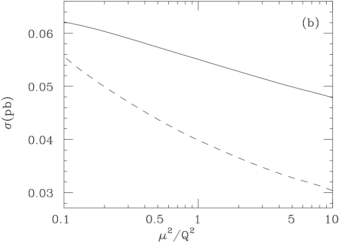
Figure 3: The two-jet cross section at high $Q^{2}$ in the HERA lab frame at LO (dashed) and NLO (solid) in the CDF cone algorithm (a), the improved cone algorithm (b) and the $k_{\perp}$ algorithm (c). Taken from $\!{}^{{\bf?}}$.

The results in the iterative cone algorithm are clearly out of control, while those in the improved cone algorithm are considerably better. It is worth noting that the $k_{\perp}$ algorithm, to be discussed shortly, is better behaved still. Similar results were found by the jets working group of the Physics at Run II workshop$\!{}^{{\bf?}}$.

The Improved Legacy Cone Algorithm

A recent innovation arising from the Physics at Run II workshop is a new accord on how to define cone jets, the ILCA, based on the improvement suggested in Ref. $\!{}^{{\bf?},{\bf?}}$.

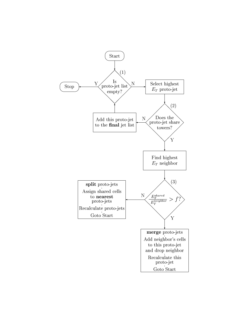
Figure 4: The full specification of the Improved Legacy Cone Algorithm. Taken from $\!{}^{{\bf?}}$.

As shown in Fig. 4 (Figs. 4, 5 and 18 of $\!{}^{{\bf?}}$) it is fully algorithmic, if a little cumbersome, meaning that any experiment or theorist can implement it in exactly the same way. Among the requirements it had to fulfil is that its numerical result be within 5% of the algorithms used by CDF and D0 in Run I, which is the case. Despite this small difference at the hadron level, it is finite order-by-order in perturbation theory and has smaller hadronization corrections. It is therefore a significant step forwards.

2.2 The $k_{\perp}$ cluster algorithm

Despite the improvements in the cone algorithm, it still has problems relative to the $k_{\perp}$ cluster algorithm$\!{}^{{\bf?},{\bf?}}$.

Figure 5: The full specification of the inclusive $k_{\perp}$ algorithm. Taken from $\!{}^{{\bf?}}$.

The definition of this is shown in Fig. 5 (Fig. 19 of $\!{}^{{\bf?}}$) in the same notation: it is clearly much simpler. Its results depend on an input parameter $R$ (sometimes called $D$), which actually plays a similar role to the radius parameter in the cone algorithm. Among its advantages are its simplicity, the fact that it exhaustively maps every hadron in the final state to one and only one jet with no overlaps, and the fact that it is based on the $k_{\perp}$ measure, allowing the phase space for sequential soft gluon emission to be factorized and the corresponding large logarithms to be summed to all orders. It also suffers smaller hadronization and detector corrections than the cone algorithm in practice.

As shown in Fig. 6 (Fig. 2b of $\!{}^{{\bf?}}$), at the level of the NLO inclusive jet cross section, the two jet definitions are essentially identical.

Figure 6: Order $\alpha_{s}^{3}$ inclusive jet cross section for $E_{T}=100$ GeV, $\sqrt{s}=1800$ GeV averaged over $\eta_{J}$ in the range $0.1<|\eta_{J}|<0.7$. The pairs of curves corresponding to the two algorithms are: $\mu=E_{T}$ (solid), $\mu=E_{T}/2$ (dot-dash), $\mu=E_{T}/4$ (dot-dot-dot-dash) plotted against $R^{\prime}=1.35R_{cone}$ for the cone algorithm and against $R^{\prime}=R_{comb}$ for the $k_{\perp}$ algorithm. Taken from $\!{}^{{\bf?}}$.

However, even at that order the energy spread within the jet is quite different, as shown in Fig. 7 (Fig. 1 of $\!{}^{{\bf?}}$).

Figure 7: The fraction of jet $E_{T}$ in angular annuli $r$ to $r+0.1$ comparing the cone and $k_{\perp}$ (“comb”) jet algorithms. In both cases the jet has $R=1.0$, $E_{T}=100$ GeV, $\sqrt{s}=1800$ GeV, $0.1<|\eta_{J}|<0.7$ and renormalization/factorization scale $\mu=E_{T}/2$. Taken from $\!{}^{{\bf?}}$.

The cluster algorithm pays more attention to the core of the jet, while the local optimization inherent in the cone algorithm does its best to suck as much soft junk into the edges of the jet as possible. This is thought to be why the cluster algorithm gives significantly cleaner reconstruction of highly boosted objects as shown in Fig. 8 (Fig. 1b of $\!{}^{{\bf?}}$).

Figure 8: Reconstructed mass distribution of Higgs candidates (with a fixed Higgs mass of 600 GeV) according to the cluster (solid and dashed) and cone (dotted and dot-dashed) algorithms, at calorimeter level with (solid and dotted) and without (dashed and dot-dashed) particles from the underlying event. Taken from $\!{}^{{\bf?}}$.

Both H1 and ZEUS now use the $k_{\perp}$ algorithm as their ‘algorithm of choice’, and CDF and D0 are planning to use it on an equal footing with the ILCA in Run II.

Preclustering

One small problem with the $k_{\perp}$ algorithm that has yet to be solved is the possible need for a preclustering step. This is needed by the Tevatron experiments for several reasons.

Firstly in D0 some calorimeter cells have negative energy, and it is not entirely clear whether these can be incorporated into the algorithm (although it is not clear to me that they cannot, for example by replacing $E_{Ti}^{2}$ by

$$E^{\prime 2}_{Ti}\equiv E_{Ti}^{2}\times\mathrm{sign}(E_{ti}).$$ (4)

These negative energy cells would then always be clustered with their nearest neighbours in a process that would always continue until there are no negative energy clusters left, regardless of the jet resolution criterion).

Secondly, due to calorimeter segmentation and the finite transverse size of hadronic showers, it is possible for one hadron to produce two or more non-zero energy cells, or for two hadrons to shower into a single cell. Preclustering reduces the size of the detector corrections associated with these effects, particularly at small subjet resolution scales.

Finally, the clustering process takes ${\cal{O}}(n^{3})$ time, where $n$ is the number of initial momenta. For Tevatron events this time can be prohibitive if all calorimeter cells are used as input. It can be reduced considerably by a little preclustering$\!{}^{{\bf?}}$.

Unfortunately no theoretical implementation of preclustering has been proposed as yet. It is not even clear whether it is possible to satisfy the experimental needs with a theoretically-calculable algorithm. A possible solution is to run the inclusive $k_{\perp}$ algorithm with a small $R$ parameter, $R\sim 0.1\!-0.2$, and to use the output of this algorithm as an input to the main algorithm. It seems likely that the large logarithms associated with this could be summed to all orders, but it has not been explicitly checked. Clearly it does not solve the problem of cpu time, so is not a complete solution, but if it could be shown that this has similar results to the experimental algorithm with the same precluster radius then it could be used as a common ground on which to compare theory and experiment. That is, one could correct the experimentally-preclustered calorimeter-level results to theoretically-preclustered hadron level, rather than all the way to un-preclustered hadron level.

3 Jet structure

3.1 Jet shape

The classic way to study the internal structure of jets is with the jet shape. This is inspired by the cone algorithm, although its use is not limited to cone jets. The jet shape $\Psi(r)$ is defined as the fraction of the jet’s energy contained in a cone of radius $r$ centred on its direction. We therefore have $\Psi(R)\sim 1$, meaning that the jet’s energy is all contained within a cone of radius $R$ (the relation is not exact because in neither the cluster algorithm, nor even the cone algorithm after the merging/splitting step, is the edge of a jet an exact geometric cone). Narrower jets are characterized by larger values of $\Psi(r)$. The jet shape is sometimes discussed in terms of the energy fractions in concentric angular annuli, $\rho(r)\equiv-\mathrm{d}\Psi/\mathrm{d}r$.

It has long been known that parton shower Monte Carlo programs like HERWIG predict considerably narrower jets than are observed in the Tevatron data, for example Fig. 9 (Fig. 1 of $\!{}^{{\bf?}}$).

Figure 9: The average integrated $E_{T}$ fraction versus the subcone radius is plotted for the data and HERWIG Monte Carlo program, at calorimeter level, for the $E_{T}$ range 45–70 GeV. Taken from $\!{}^{{\bf?}}$.

Since jet shapes in $\mathrm{e^{+}e^{-}}$ annihilation were known to be well described, even when separated out into quark- and gluon-jet samples$\!{}^{{\bf?}}$, possible explanations focused on the two main new ingredients in hadron collisions, initial-state radiation (ISR) and the underlying event. The ISR model is well tested by the Tevatron experiments’ measurements of colour coherence effects in two-jet events, which HERWIG describes well$\!{}^{{\bf?}}$. This leaves underlying event effects as the most likely culprit.

This hypothesis can be tested at HERA, since resolved photoproduction should have an underlying event and direct photoproduction and DIS should not. A great deal of excellent data have appeared in the last couple of years$\!{}^{{\bf?},{\bf?},{\bf?}}$, from which we choose just one example, dijet events in DIS from H1, Fig. 10 (Fig. 5 of $\!{}^{{\bf?}}$).

Figure 10: The jet shapes for the inclusive $k_{\perp}$ algorithm. The data are shown as a function of the transverse jet energy and the jet pseudo-rapidity in the Breit frame. The results are compared to predictions of QCD models. Taken from $\!{}^{{\bf?}}$.

It can be seen that HERWIG’s prediction is again too narrow, although by much less than at the Tevatron. Since there should be no underlying event correction, this clearly needs to be understood in more detail. It is worth noting that in this kinematic region the hadronization corrections are huge, as shown in Fig. 11 (Fig. 6a of $\!{}^{{\bf?}}$) for the LEPTO generator.

Figure 11: Model predictions of the jet shape for the inclusive $k_{\perp}$ algorithm from the LEPTO parton shower model. The jet shapes are shown separately for quark and gluon induced jets with $E_{T,\mathrm{Breit}}>8$ GeV and $\eta_{\mathrm{Breit}}<1.5$ together with the sum of both and the comparison to the H1 measurement. The distribution before hadronization is also shown. Taken from $\!{}^{{\bf?}}$.

As mentioned earlier, DIS in the HERA lab frame has a special role in jet physics because the recoiling electron acts kinematically like a parton but is not coloured. This has enabled the first NLO calculation of the jet shape to be made$\!{}^{{\bf?}}$.

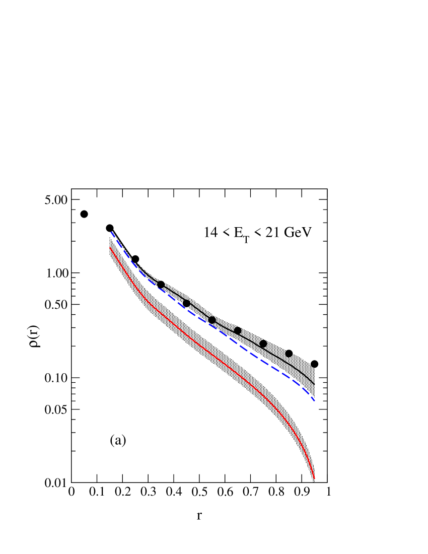
Figure 12: Comparison of ZEUS jet shape data $\!{}^{{\bf?}}$ with QCD predictions for DIS jets reconstructed by the iterative cone algorithm. Jet cuts are: $-1<\eta<2$ and 14 GeV${}<E_{T}<{}$21 GeV. ZEUS data (circles) are compared with LO (lower band) and NLO (dashed line) QCD predictions. The upper band represents the NLO jet shape with additional cuts that are not made on the data. The width of the bands corresponds to varying the renormalization scale between $\mu_{r}^{2}=\alpha_{s}Q^{2}/4$ and $\mu_{r}^{2}=4\alpha_{s}Q^{2}$. Taken from $\!{}^{{\bf?}}$.

A comparison with ZEUS data is shown in Fig. 12 (Fig. 4a of $\!{}^{{\bf?}}$). For precisely the reasons mentioned earlier this is extremely sensitive to the details of the jet algorithm. Since the iterative algorithm used by the ZEUS experiment is not infrared safe, it cannot be used in the NLO calculation, so this comparison can only be taken as indicative. To supposedly take account of this, the authors of $\!{}^{{\bf?}}$ applied an additional cut in the calculation that was not applied to the data and chose a very small scale for the running coupling. Bearing this in mind, and the fact that the hadronization corrections shown in Fig. 11 (Fig. 6a of $\!{}^{{\bf?}}$) are about a factor of two, the claimed good agreement shown in Fig. 12 (Fig. 4a of $\!{}^{{\bf?}}$) must be seen as coincidental.

3.2 Subjet studies

The $k_{\perp}$ algorithm naturally suggests a new way of analysing the internal structure of jets that is much closer to the partonic picture of how that structure arises. After identifying a jet of a given $E_{T}$, we rerun the $k_{\perp}$ algorithm, but only on those particles that were assigned to this jet. We stop clustering when all values of $d_{ij}$ satisfy $d_{ij}>y_{\mathrm{cut}}E_{T}^{2}$, namely when all internal relative transverse momenta are greater than $\sqrt{y_{\mathrm{cut}}}E_{T}$. Analysing the jets in this way is extremely similar to analysing $\mathrm{e^{+}e^{-}}$ annihilation events at $\sqrt{s}=E_{T}$ and the same value of $y_{\mathrm{cut}}$ and in fact it can be shown$\!{}^{{\bf?}}$ that the leading logarithms are identical. Even the ISR of gluons into the jet, which contributes at next-to-leading logarithmic accuracy, can be summed to all orders and results are shown in Fig. 13 (Fig. 1 of $\!{}^{{\bf?}}$) for the average number of subjets.

Figure 13: The multiplicity of subjets in a 100 GeV jet according to the leading-order matrix element (dashed), matched leading-order and final-state logs (dot-dashed) and the full result with matched leading-order and leading and next-to-leading logs (solid). Taken from $\!{}^{{\bf?}}$.

The resummation can be seen to be extremely important for small $y_{\mathrm{cut}}$, while the initial-state resummation is only a relatively small correction.

The subjet multiplicity was studied in a preliminary way by D0 in $\!{}^{{\bf?}}$ and compared with the parton shower Monte Carlo programs. The results are shown in Fig. 14 (Fig. 7 of $\!{}^{{\bf?}}$).

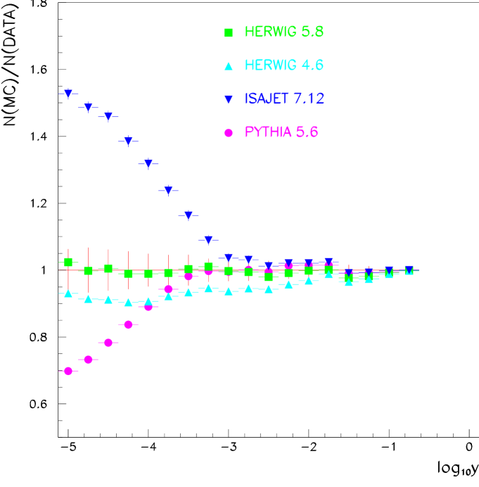
Figure 14: The multiplicity of subjets in jets of at least 250 GeV $E_{T}$: the predictions of various Monte Carlo models are divided by the data. The error bars on the central line are those of the data. Taken from $\!{}^{{\bf?}}$.

I still find this figure amazing: on the left-hand side we are studying 250 GeV jets at a scale of less than 1 GeV where the hadronization corrections are huge and, at least in HERWIG, the description is perfect. It is possible that the over-production of subjets in ISAJET is related to the lack of colour coherence and angular ordering and that the deficit in PYTHIA, which starts at smaller $y_{\mathrm{cut}}$ is due to an over-estimate of the amount of ‘string drag’ pulling soft hadrons out of the jet, although these effects have not been studied in detail.

Subjet properties have also been studied for separate quark and gluon jet samples using an extremely neat statistical separation$\!{}^{{\bf?}}$. On the assumption that quark and gluon jet properties are each independent of $\sqrt{s}$ for fixed $E_{T}$, the fact that the flavour mix of jets varies strongly and that this variation is well predicted by perturbative QCD can be used to measure their individual properties without the need for an event-by-event tag.

Figure 15: Corrected subjet multiplicity in quark and gluon jets, extracted from D0 data. Taken from $\!{}^{{\bf?}}$.

The results for the subjet rates are shown in Fig. 15 (Fig. 3 of $\!{}^{{\bf?}}$), where it can be seen that as expected gluon jets contain a lot more activity than quark jets. The distributions are again well described by HERWIG.

All-orders resummation for subjet rates

Recently the first calculation of subjet rates in hadron collisions was performed$\!{}^{{\bf?}}$. In general the $n$-subjet rate contains terms like $\alpha_{s}^{m}\log^{2m}y_{\mathrm{cut}}$ at all orders of perturbation theory $m\geq n\!-\!1$. Together with the next-to-leading logarithms ($\alpha_{s}^{m}\log^{2m-1}y_{\mathrm{cut}}$) these can be summed to all orders using the same trick as was used for the subjet multiplicity in $\!{}^{{\bf?}}$, which is illustrated in Fig. 16.

Figure 16: Illustration of the calculations of Refs. $\!{}^{{\bf?},{\bf?}}$. The primary hard parton evolves due to final state radiation and its double logs give the leading log contribution. It is accounted for to next-to-leading logarithmic accuracy. Soft initial state radiation can also be clustered into the jet and its double logs contribute to the next-to-leading logs. It only needs to be calculated to leading log accuracy since it is already one log down. This is done by multiplying the exact hard matrix element by a soft gluon multiplication factor.

The evolution of the final-state jet is process-independent and can be summed to next-to-leading log accuracy using the well-known formulæ from $\mathrm{e^{+}e^{-}}$ annihilation$\!{}^{{\bf?}}$. However, the next-to-leading logs also receive a contribution from soft initial-state radiation that happens to be close enough to the jet to be combined with it. As the probability of such emission depends on the full details of the hard process through the kinematics, identities and colour-connection of all participating partons, it seems unlikely that this could be resummed analytically. However, by carefully combining the analytical result with a numerical integration of the exact matrix element to produce one additional gluon, it is possible not only to sum these logs to all orders, but also to automatically exactly reproduce the ${\cal{O}}(\alpha_{s})$ contribution to the one- and two-subjet rates.

Examples of the results are shown in Figs. 17 and 18 (Figs. 9, 10 and 12 of $\!{}^{{\bf?}}$). The first thing to note is that the general forms look very reminiscent of $\mathrm{e^{+}e^{-}}$ annihilation. It is possible to separate out the contribution from quark and gluon jets and test the hypothesis used by D0 that these are independent of the centre-of-mass collision energy.

Figure 17: $y_{\mathrm{cut}}$ dependence of the $N$ subjet rate in quark (solid) and gluon (dashed) jets for $N=1$, 2, 3, 4 and $\geq 5$ at $\sqrt{s}=1800$ GeV. Also shown (dotted) are the same things at $\sqrt{s}=630$ GeV. Adapted from $\!{}^{{\bf?}}$.

As can be seen in Fig. 17 (Figs. 9 and 10 of $\!{}^{{\bf?}}$) this is the case.

Figure 18: Rates for $N$ subjets at $y_{\mathrm{cut}}=10^{-3}$ in quark (crosses) and gluon (circles) jets. Taken from $\!{}^{{\bf?}}$.

The results at fixed $y_{\mathrm{cut}}$ shown in Fig. 18 (Fig. 12 of $\!{}^{{\bf?}}$) are certainly reminiscent of D0’s but, owing to the fact mentioned earlier that they use a preclustering algorithm and the theoretical calculation does not, direct comparison is not yet possible.

It is worth noting that in order to extend this calculation to DIS or photoproduction, it is necessary only to put the appropriate matrix element into the box marked “exact ${\cal{O}}(\alpha_{s}^{3})$” in Fig. 16. All the analytically-summed contributions are then identical.

4 Conclusion

Precision QCD physics, and the use of jets in precision electroweak physics, requires reliable jet definitions and reliable predictions of the internal structure of jets. We have reviewed a small subset of the advances made in these areas in recent years.

References

References

- [1] CDF Collaboration, Phys. Rev. D45 (1992) 1448.
- [2] W.T. Giele and W.B. Kilgore, Phys. Rev. D55 (1997) 7183 [hep-ph/9610433].
- [3] M.H. Seymour, Nucl. Phys. B513 (1998) 269 [hep-ph/9707338].
- [4] S.D. Ellis, D.E. Soper and H.-C. Yang, unpublished, 1993.
- [5] B. Pötter and M.H. Seymour, J. Phys. G25 (1999) 1473.
- [6] G.C. Blazey et al., “Run II jet physics”, hep-ex/0005012.
- [7] S. Catani, Yu.L. Dokshitzer, M.H. Seymour and B.R. Webber, Nucl. Phys. B406 (1993) 187.
- [8] S.D. Ellis and D.E. Soper, Phys. Rev. D48 (1993) 3160 [hep-ph/9305266].
- [9] M.H. Seymour, Z. Phys. C62 (1994) 127.
- [10] D0 Collaboration, Phys. Lett. B357 (1995) 500.
- [11] OPAL Collaboration, Z. Phys. C69 (1996) 543.
- [12] CDF Collaboration, Phys. Rev. D50 (1994) 5562.
- [13] H1 Collaboration, Nucl. Phys. B545 (1999) 3 [hep-ex/9901010].
- [14] ZEUS Collaboration, Eur. Phys. J. C8 (1999) 367 [hep-ex/9804001].
-
[15]
J. Terron, J. Phys. G G25 (1999) 1365
[hep-ex/9903049].
ZEUS Collaboration, Eur. Phys. J. C2 (1998) 61 [hep-ex/9710002]. - [16] N. Kauer, L. Reina, J. Repond and D. Zeppenfeld, Phys. Lett. B460 (1999) 189 [hep-ph/9904500].
- [17] M.H. Seymour, Nucl. Phys. B421 (1994) 545.
- [18] R.V. Astur, ‘Studies of Jet Structure at the Tevatron’, Proc. 10th Topical Workshop on Proton–Antiproton Collider Physics, 1995, eds. R. Raja and J. Yoh, p. 598.
- [19] D0 Collaboration, Nucl. Phys. Proc. Suppl. 79 (1999) 494 [hep-ex/9907059].
- [20] J.R. Forshaw and M.H. Seymour, JHEP 9909 (1999) 009 [hep-ph/9908307].
- [21] S. Catani, Yu.L. Dokshitzer, F. Fiorani and B.R. Webber, Nucl. Phys. B377 (1992) 445.