Field distributions in heavy mesons and baryons

Abstract

Field distributions generated by static $Q\bar{Q}$ and $QQQ$ sources are calculated analytically in the framework of the Field Correlator Method (FCM) using Gaussian (bilocal) correlator. In both cases the string consists mostly of longitudinal color electric field, while transverse electric field contributes locally less then 3%, in agreement with earlier lattice studies. In the $QQQ$ case the profile of the $Y$ shape was calculated for the first time and found to have a complicated structure with a deep well at the string junction position. Possible consequences of this form for the baryon structure are discussed.

1 Introduction

Field distributions inside the string connecting static $Q\bar{Q}$ sources have been measured repeatedly on the lattice using both connected [1-3] and disconnected [4, 5] probes. Similar measurements were done later also for Abelian projected configurations [6]. Analytic calculations for the disconnected probe made in [7] in the framework of the Gaussian approximation to the FCM [8, 9] have revealed a clear string-like structure of the same type as was found on the lattice.

However the connected probe yields an independent and more direct information on the field distribution in the string as compared to the disconnected one, namely the expectation values of the fields themselves rather then that of field squares.

A detailed comparison of lattice data [1] with analytic predictions of FCM was done in [2], demonstrating a remarkable agreement in all distributions. In particular, the measured decrease of longitudinal electric field $E_{\parallel}$ with distance from the string axis (”the string profile”) agrees remarkably well with the contribution of the lowest, (bilocal) correlator [2]. It should be noted that the input of FCM is the field correlator as a function of distance, which is taken from the lattice measurements [10], yielding an exponential form of both scalar formfactors $D$ and $D_{1}$ [8] with the slope $T_{g}\approx 0.2$fm. The dominance of the bilocal correlator (sometimes called the Gaussian Stochastic Model (GSM) of the QCD vacuum) was verified recently on the lattice by the precision measurement of Wilson loops (static potentials) in different SU(3) representations [11]. Analysis of data [11] made in [12] has demonstrated that GSM contribution around 99% to the static $Q\bar{Q}$ potential is consistent with the data.

These results give an additional stimulus to the analytic calculation of field distributions using lowest bilocal correlator. Our purpose in this letter is to calculate $3d$ field distributions to demonstrate the string formation, and in particular to study transverse electric fields and nonconfining piece $(D_{1})$ of the bilocal correlator which was not done in [2]. In addition we calculate for the first time the field distributions in the static $QQQ$ system as a function of distance between quarks forming an equilateral triangle. It will be shown that for the lowest energy configuration (the so-called $Y$-shaped, or string-junction configuration) the field distribution has a rather peculiar ”well” form and vanishes at the place of the string-junction. The analysis of equations reveals the reason of such shape, and yields an estimate of the well size.

The plan of the paper is as follows. In section 2 necessary formulas are derived in the framework of FCM for the connected-probe field distributions. The $Q\bar{Q}$ case is treated in detail and $3d$ distributions are given. In section 3 the $QQQ$ case is considered and the relief of the $Y$-shaped string with the well is given. In section 4 the $3Q$ potential is derived and compared with lattice measurements. In conclusion possible physical consequences and relation to the real case of heavy and light hadrons are discussed.

2 $Q\bar{Q}$ case

We follow in this section notations and methods used previously in [2]. A gauge invariant connected probe $\rho_{\mu\nu}(x)$ is made with the infinitesimal plaquette $P_{\mu\nu}$ at the point $x$, connected by parallel transporters (Schwinger lines) $L$, $L^{+}$ to the contour $C$ of the Wilson loop $W$ as shown in Fig.1.

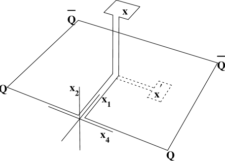
Figure 1: A connected probe in the $Q\bar{Q}$ case.

$$\rho_{\mu\nu}(x)=\frac{\langle\mathrm{tr}(WLP_{\mu\nu}(x)L^{+})\rangle}{\langle\mathrm{tr}W\rangle}-1\equiv\langle P_{\mu\nu}(x)\rangle_{Q\bar{Q}}.$$ (1)

Schwinger lines contribution to probe depends on their length and shape and is minimal when they are taken to be straight lines as shown in Fig.1. When the size $a$ of the plaquette $P_{\mu\nu}$ tends to zero one has

$$\langle P_{\mu\nu}(x)\rangle_{Q\bar{Q}}\to a^{2}\langle F_{\mu\nu}(x)\rangle_{Q\bar{Q}}.$$ (2)

To calculate (1) one can use the cluster expansion theorem [8] applied to the complex Wilson loop $\bar{C}$ consisting of the original contour $C$ and the plaquette $P_{\mu\nu}$ attached with the lines $L,L^{+}$. In the Gaussian (bilocal) approximation one can proceed as in [2] to obtain the final result for the contribution of the lowest correlator, $\langle FF\rangle$,

$$\rho_{\mu\nu}(x)=a^{2}\int_{S(C)}d\sigma_{\rho\lambda}(x^{\prime})D_{\rho\lambda,\mu\nu}(x^{\prime},x)+O(a^{4}).$$ (3)

Here $S(C)$ is the minimal area surface inside the contour $C$, and $D$ is

$$D_{\rho\lambda,\mu\nu}(x^{\prime},x)=\frac{g^{2}}{N_{c}}\mathrm{tr}\langle F_{\rho\lambda}(x^{\prime})\Phi(x^{\prime},x)F_{\mu\nu}(x)\Phi(x,x^{\prime})\rangle,$$ (4)

while $\Phi(x,y)$ is the parallel transporter, connecting points $x,y$. Integration goes over infinitesimal plaquettes $\Delta\sigma_{\rho\lambda}(x^{\prime})$ on the surface $S$ as depicted in Fig.1 by dashed line. For the gauge-invariant function $D_{\rho\lambda,\mu\nu}$ there exists an expression in terms of two scalar functions $D$ and $D_{1}$ (see second ref. in [8]),

$$D_{\rho\lambda,\mu\nu}(x,y)=(\delta_{\rho\mu}\delta_{\lambda\nu}-\delta_{\rho\nu}\delta_{\mu\lambda})D(h)+$$

$$\frac{1}{2}[\frac{\partial}{\partial h_{\rho}}h_{\mu}\delta_{\lambda\nu}-\frac{\partial}{\partial h_{\lambda}}h_{\mu}\delta_{\rho\nu}+\rho\lambda\leftrightarrow\mu\nu]D_{1}(h),$$ (5)

where $h\equiv x-y$. The functions $D,D_{1}$ have been measured on the lattice [10] and were found to have an exponential form beyond $x=0.1$fm.

Here we use the exponential ansatz in the whole region of $x$, as it was done previously in [2], with parameters as in [10],[2]

$$D(x)=D(0)\exp(-\mu|x|),~{}~{}D_{1}(x)=D_{1}(0)\exp(-\mu|x|),$$ (6)

$$D_{1}(0)\approx\frac{1}{3}D(0),~{}~{}\mu\approx 1\mathrm{GeV}.$$

In the same Gaussian approximation, i.e. neglecting all higher correlators (which is consistent with lattice measurements of static potentials with accuracy of better than one percent [11, 12]) $D(0)$ can be expressed through the string tension

$$\sigma=\frac{1}{2}\int D(x)d^{2}x=\pi D(0)/\mu^{2}.$$ (7)

This connection will be important in what follows for the correct normalization of the field distribution in $Q\bar{Q}$ and $QQQ$.

To proceed with the integration in (3), choose the coordinate axes as shown in Fig.1. The contour $C$ of the Wilson loop is a rectangular of size $R\times T$ where $R$ is quark separation and $T$ is temporal extension of the Wilson loop. Plaquettes $\Delta\sigma_{\rho\lambda}(x^{\prime})$, $x^{\prime}=(x_{1}^{\prime},x_{2}^{\prime},x_{3}^{\prime},x_{4}^{\prime})$, have coordinates $0\leq x_{1}^{\prime}\leq R,x_{2}^{\prime}=x_{3}^{\prime}=0,-T/2\leq x_{4}^{\prime}\leq T/2$. The probe is placed at $x=(x_{1},x_{2},x_{3},x_{4})$. $x_{1}$ is the coordinate of the probe along string axis, $x_{2}$ is the distance from the probe to the string axis, $x_{3}=x_{4}=0$. The only nonzero components of color field are electric ones in $x_{1}$ and $x_{2}$ directions (see [2] for symmetry arguments and discussion). The resulting equations are directly obtained from (2-5) ($\rho_{i4}(x_{1},x_{2})=a^{2}\langle E_{i}(x_{1},x_{2})\rangle_{Q\bar{Q}}\equiv a^{2}E_{i}(x_{1},x_{2})$):

$$E_{1}(x_{1},x_{2})=\int^{R}_{0}dx^{\prime}_{1}\int^{\frac{T}{2}}_{-\frac{T}{2}}dx^{\prime}_{4}[D(0)+D_{1}(0)-\mu\frac{h^{2}_{4}+h^{2}_{1}}{2h}D_{1}(0)]e^{-\mu h},$$ (8)

$$E_{2}(x_{1},x_{2})=-\mu x_{2}\int^{R}_{0}dx^{\prime}_{1}\int^{\frac{T}{2}}_{-\frac{T}{2}}dx^{\prime}_{4}\frac{(x_{1}-x^{\prime}_{1})}{2h}D_{1}(0)e^{-\mu h}.$$ (9)

Here we have defined

$$h_{4}=-x^{\prime}_{4},~{}~{}h_{1}=x_{1}-x^{\prime}_{1};~{}~{}h^{2}=h^{2}_{4}+h^{2}_{1}+x^{2}_{2}.$$ (10)

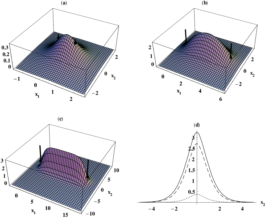
Figure 2: Distribution of the field $E_{1}^{2}$ measured in GeV²/fm² around static $Q\bar{Q}$ sources as function of $x_{1}$ (distance along the string) and $x_{2}$ (distance from the string axis). Both distances are measured in units of $T_{g}$. Positions of $Q$ and $\bar{Q}$ are marked with points with vertical lines. The cases (a),(b),(c) refer to the interquark distances $R_{Q\bar{Q}}=1,5$ and $15T_{g}$. In Fig.2(d) the string profile (i.e. $E_{1}^{2}(x_{2})$ distribution at the middle of the string) is shown, dotted, dashed and solid lines for the three interquark distances of Figs. 2(a), (b) and (c) respectively. Note the saturation of the string height and width at around $R\approx 5T_{g}$.

The field distributions $E^{2}_{1}(x_{1},x_{2})$ are shown in Fig.2 (a-c) for different quark separations, $R=T_{g},5T_{g}$ and $15T_{g}$. The string profile, i.e. $E^{2}_{1}(x_{2})$ distribution in the middle of the string, for these quark separations is shown in Fig.2 (d). One can see a clear string-like formation with the width of $2.2T_{g}$. The value of $E_{1}$ in the middle of the string does not depend on $R$ for $R>5T_{g}$. The saturated value is $E^{sat}=1.8$GeV/fm.

The field distribution $E_{2}(x_{1},x_{2})$ is shown in Fig.3 for $R=15T_{g}$. Note that $|E_{2}|$ is much smaller than $|E_{1}|,\max|E_{2}(x_{1},x_{2})|\approx 0.03\max|E_{1}(x_{1},x_{2})|$.

The distribution $E_{1}(x_{1},x_{2})$ generated by $D_{1}(x)$ is shown separately in Fig.4. One can see that $D_{1}$ does not produce a string, which is in agreement with the fact, that $D_{1}$ does not contribute to the string tension (7).

3 $QQQ$ case

In case of the $QQQ$ system the contour $C$ consists of three contours connected by the string-junction trajectory, as depicted in Fig.5. The surface $S$ consists of three surfaces $\Sigma_{A},\Sigma_{B}$ and $\Sigma_{C}$, and the probing plaquette $P_{\mu\nu}$ is attached by Schwinger lines $L,L^{+}$ to one of the static quark trajectories.

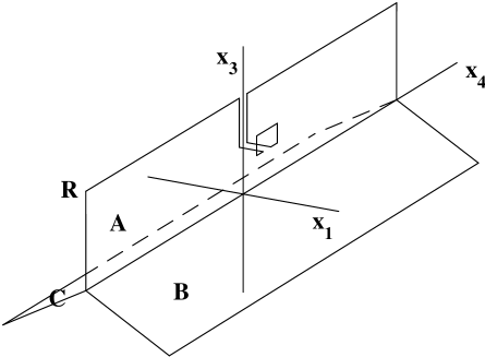
Figure 5: A connected probe in the $QQQ$ case.

Choosing the axes as shown in Fig.5, $x_{2}=0$, one has two main contributing correlators $D_{14,14}$ and $D_{34,34}$ and a subleading nondiagonal one $D_{14,34}=D_{34,14}$. As a result one obtains the following field distributions (choosing $x_{4}=0$ for the plaquette $P_{\mu\nu}$ as in the $Q\bar{Q}$ case):

$$E^{(3Q)}_{1}(x_{1},x_{3})=\int(d\sigma_{A}\Lambda^{(A)}_{14}+d\sigma_{B}\Lambda_{14}^{(B)}+d\sigma_{C}\Lambda^{(C)}_{14}),$$ (11)

$$E^{(3Q)}_{3}(x_{1},x_{3})=\int(d\sigma_{A}\Lambda^{(A)}_{34}+d\sigma_{B}\Lambda_{34}^{(B)}+d\sigma_{C}\Lambda^{(C)}_{34}),$$ (12)

where we have defined

$$d\sigma_{A}\Lambda^{(A)}_{14}=dx^{\prime}_{4}dx^{\prime}_{3}D_{34,14}(x-x^{\prime}),$$ (13)

$$d\sigma_{B}\Lambda^{(B)}_{14}=\frac{\sqrt{3}}{2}dx^{\prime}_{4}dl^{\prime}D_{14,14}-\frac{1}{2}dx^{\prime}_{4}dl^{\prime}D_{34,14},$$ (14)

$$d\sigma_{C}\Lambda^{(C)}_{14}=-\frac{\sqrt{3}}{2}dx^{\prime}_{4}dl^{\prime}D_{14,14}-\frac{1}{2}dx^{\prime}_{4}dl^{\prime}D_{34,14},$$ (15)

$$d\sigma_{A}\Lambda^{(A)}_{34}=dx^{\prime}_{4}dx^{\prime}_{3}D_{34,34}(x-x^{\prime}),$$ (16)

$$d\sigma_{B}\Lambda^{(B)}_{34}=\frac{\sqrt{3}}{2}dx^{\prime}_{4}dl^{\prime}D_{14,34}-\frac{1}{2}dx^{\prime}_{4}dl^{\prime}D_{34,34},$$ (17)

$$d\sigma_{C}\Lambda^{(C)}_{34}=-\frac{\sqrt{3}}{2}dx^{\prime}_{4}dl^{\prime}D_{14,34}-\frac{1}{2}dx^{\prime}_{4}dl^{\prime}D_{34,34}.$$ (18)

Here $dl^{\prime}$ denotes integration from $l^{\prime}=0$ to $l^{\prime}=R$, $R$ is quark separation from the string junction; $dx_{4}^{\prime}$ denotes integration from $x_{4}^{\prime}=-T/2$ to $x_{4}^{\prime}=T/2$.

Using (5) the correlators entering (13-18) can be expressed through $D,D_{1}$ as

$$D_{14,14}(z)=D(z)+D_{1}(z)+(z^{2}_{1}+z^{2}_{4})\frac{dD_{1}}{dz^{2}},$$ (19)

$$D_{34,34}(z)=D(z)+D_{1}(z)+(z^{2}_{3}+z^{2}_{4})\frac{dD_{1}}{dz^{2}},$$ (20)

$$D_{14,34}(z)=D_{34,14}(z)=z_{1}z_{3}\frac{dD_{1}}{dz^{2}}.$$ (21)

From the symmetry of Fig.5 it is clear, that the resulting field distribution is symmetric under rotation in the $(x_{3},x_{1})$ plane over angle $\frac{2\pi n}{3},~{}~{}n=0,1,2,...$ , and indeed from (11-21) one can conclude that color electric field has this symmetry.

We have calculated the $\mbox{\boldmath${\rm E}$}^{2}(\mbox{\boldmath${\rm r}$}^{2})=(E^{(3Q)}_{1})^{2}+(E^{(3Q)}_{3})^{2}$ distribution, where $\mbox{\boldmath${\rm r}$}=(x_{1},x_{3}),$ displayed on Fig.6 (a-c) for $R=T_{g},5T_{g}$ and $15T_{g}$ respectively. One can easily see the symmetry discussed above and in addition a remarkable feature - a well in $\mbox{\boldmath${\rm E}$}^{2}(\mbox{\boldmath${\rm r}$}^{2})$ near $\mbox{\boldmath${\rm r}$}=0$. The well profile, i.e. distribution of $\mbox{\boldmath${\rm E}$}^{2}$ along the $x_{3}$ axis, is depicted in Fig.6 (d) for given quark separations. As one can see, the well shape does not depend on the quark separation. At separation $15T_{g}$ the string acquires its saturation value $E^{sat}=1.8$GeV/fm. The radius of the well, i.e. distance from the string junction to the position at which $\mbox{\boldmath${\rm E}$}^{2}$ is half of its saturation value, is $1.75T_{g}$.

The physical origin of this well is understandable: the fields ${\rm E}$ are directed in three sheets $\Sigma_{A},\Sigma_{B},\Sigma_{C}$ and are perpendicular to the string-junction line; hence there is no preferred direction for the field ${\rm E}$ at $\mbox{\boldmath${\rm r}$}=0$. To get more quantitative insight into the problem, let us consider the line $x_{1}=0$ in the plane $(x_{1},x_{3})$ and compute $E_{1}^{(3Q)}$ and $E^{(3Q)}_{3}$ as functions of $x_{3}$. From (11), (12) one immediately obtains

$$E^{(3Q)}_{1}(x_{1}=0,x_{3})=0,$$ (22)

$$E^{(3Q)}_{3}(x_{1}=0,x_{3})=\int^{\frac{T}{2}}_{-\frac{T}{2}}dx^{\prime}_{4}\int^{R}_{0}dl^{\prime}\{\tilde{D}(\sqrt{(x^{\prime}_{4})^{2}+(x_{3}-l^{\prime})^{2}})$$

$$-\tilde{D}(\sqrt{(x^{\prime}_{4})^{2}+\frac{3}{4}l^{{}^{\prime}2}+(x_{3}+\frac{1}{2}l^{\prime})^{2}})\},$$ (23)

where $\tilde{D}\equiv D_{34,34}(h)$. From (23) one can deduce that $E_{3}$ vanishes linearly at $x_{3}=0$ and grows fast for positive $x_{3}$ attaining a constant limit for $x_{3}\sim\frac{1}{\mu}$ when $R\mu\gg 1$. Thus $\mbox{\boldmath${\rm E}$}=0$ at the center of the well and the radius of the well is of the order of $r\sim\frac{1}{\mu}=T_{g}$.

Using the connected probe we have built the square of expectation value of baryon field from the expectation values of fields of Wilson loop three sheets. Let us mention that by the disconnected probe we could measure the expectation value of squared fields and would know nothing about fields themselves since in general $<E^{2}>\neq<E>^{2}$.

4 Quark interaction potential in $QQQ$ case

We now go over to another topic, closely connected with the previous one, namely the static potential for the $QQQ$ system. Choosing the same $Y$-shaped equilateral configuration one has from the cluster expansion of the Wilson loop $W^{(3Q)}$,

$$V^{(3Q)}(R)=-\lim_{T\to\infty}\frac{1}{T}\ln\langle W^{(3Q)}(R,T)\rangle=$$

$$=\sum_{a,b=A,B,C}\frac{1}{2}\int\int d\sigma_{a}(x)d\sigma_{b}(y)D_{a,b}(x,y)=\frac{1}{2}\sum_{a,b}V_{a,b}(R),$$ (24)

where, e.g.

$$V_{A,A}(R)=\frac{1}{T}\int^{\frac{T}{2}}_{-\frac{T}{2}}dt\int^{\frac{T}{2}}_{-\frac{T}{2}}dt^{\prime}\int^{R}_{0}dz\int^{R}_{0}dz^{\prime}[D(h)+D_{1}+h^{2}\frac{dD_{1}}{dh^{2}}]$$ (25)

and $h^{2}=(z-z^{\prime})^{2}+(t-t^{\prime})^{2}$.

Using (13)-(18) one can easily find the nondiagonal terms, e.g.

$$V_{A,B}(R)=\frac{1}{T}\int^{\frac{T}{2}}_{-\frac{T}{2}}dt\int^{\frac{T}{2}}_{-\frac{T}{2}}dt^{\prime}\int^{R}_{0}dl\int^{R}_{0}dl^{\prime}[\frac{\sqrt{3}}{2}D_{14,34}(\tilde{h})-\frac{1}{2}D_{34,34}(\tilde{h})],$$ (26)

where $\tilde{h}^{2}=(t-t^{\prime})^{2}+\tilde{h}^{2}_{1}+\tilde{h}^{2}_{3},~{}~{}\tilde{h}_{1}=-\frac{\sqrt{3}}{2}l^{\prime},~{}~{}\tilde{h}_{3}=l+\frac{1}{2}l^{\prime};$ and

$$D_{14,34}(\tilde{h})=\tilde{h}_{1}\tilde{h}_{3}\frac{dD_{1}(\tilde{h}^{2})}{d\tilde{h}^{2}}.$$ (27)

For $V_{A,C}(R)$ both (26) and (27) are valid, but the sign of $\tilde{h}_{1}$ is opposite to that of (27).

From symmetry of the problem it is clear that the total potential is expressed through $V_{A,A},V_{A,B},V_{A,C}$ as

$$V^{(3Q)}(R)=\frac{3}{2}(V_{A,A}+V_{A,B}+V_{A,C}).$$ (28)

We plot this potential in Fig.7 together with the total potential including the perturbative one-gluon-exchange parts,

$$V_{tot}^{(3Q)}(R)=V^{(3Q)}(R)-\frac{2\alpha_{s}}{\sqrt{3}R},$$ (29)

where $\alpha_{s}=3/4e$. $e=0.295$ from fit of the $Q\bar{Q}$ lattice potential by the Coulomb plus linear (Cornell) potential (see [13] and references therein). One can notice in Fig.7 that large-distance asymptotic of the $V^{(3Q)}(R)$ is equal to $3\sigma R$, as it should be. At $R=3.5T_{g}$ the slope of $V^{(3Q)}$ is $2.6\sigma$. This is consistent with recent lattice measurements of $V^{(3Q)}_{tot}(R)$ ([13]) fitted in the measured region $0.055$fm$\leq R\leq 0.71$fm by the Cornell potential with the same slope of linear part.

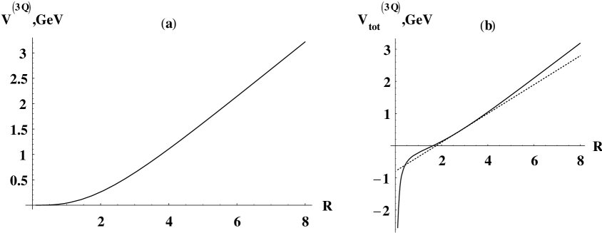
Figure 7: (a). $3Q$ potential for the string junction configuration of Fig.5 as a function of distance from quark to string junction (in units of $T_{g}$). (b). The same as in (a) with perturbative one-gluon-exchange potential added.

5 Conclusions

We have calculated connected-probe field distributions for $Q\bar{Q}$ and $QQQ$ cases using the lowest (Gaussian) field correlator. Basing on the results of [11,12], one expects that higher correlators would not significantly change our picture.

The connected-probe analysis is essential for establishing direction of fields in the string and distinguishing color-electric and color-magnetic contributions, since due to properties of the Gaussian correlator (5) the orientation of the probing plaquette $P_{\mu\nu}$ allows to fix the vector of the field in the string.

Our results for the $Q\bar{Q}$ case are in agreement with earlier calculations in [1-3]. The bulk of the string fields is also in accordance with disconnected-probe analyses [4, 5].

The QQQ results are new and striking. A deep well in the electric field distribution appears at the string-junction position. Exactly at this point electric field vanishes because of rigorous symmetry arguments. The well has a radius of $1.75T_{g}$ and implies strong suppression of fields in the middle of the heavy baryon. Since the Wilson loop for the QQQ configuration can be used to generate interaction applicable for light quarks [14], physical consequences of this suppression can be in principle observable both for light and heavy hadrons. One consequence can be seen in Fig.7, where the nonperturbative part of the potential grows very slowly at small $R$, so that the asymptotic slope is obtained only at very large distances. Therefore an effective slope for ground-state hadrons can be some 10-20% smaller, the fact which is in agreement with relativistic quark model of baryons [15] and with recent lattice calculations of static QQQ potential [13].

One should note that the vanishing of fields at the string junction holds for directed field
distribution, measured in the connected-probe analysis, and may not be true for field fluctuations, measured in the disconnected probe. This topic and other possible consequences of the field suppression in the middle of the baryon call for further investigations.

Financial support of the RFFI grants 00-02-17836 and 00-15-96786 is gratefully acknowledged.

The authors are grateful to N.O.Agasyan, A.B.Kaidalov, Yu.S.Kalashnikova, V.I.Shev-
chenko for useful remarks. D.K. is grateful to D.V.Chekin for a discussion of software details.

References

- [1] A.Di Giacomo, M.Maggiore and S.Olejnik, Phys.Lett. B236 (1990) 199; Nucl.Phys. B347 (1990) 441
- [2] L.Del Debbio, A.Di Giacomo and Yu.A.Simonov, Phys.Lett. B332 (1994) 111
- [3] P.Cea and L.Cosmai, Phys.Rev. D52 (1995) 5152
- [4] G.S.Bali, Ch.Schlichter and K.Schilling, Nucl.Phys.Proc.Suppl. 42 (1995) 273; Phys.Rev. D51 (1995) 5165
- [5] R.W.Haymaker, V.Singh, Y.Peng and J.Wosiek, Phys.Rev. D53 (1996) 389
- [6] G.S.Bali, Ch.Schlichter and K.Schilling, Nucl.Phys.Proc.Suppl. 63 (1998) 519; Prog.Theor.Phys.Suppl. 131 (1998) 645
-
[7]
M.Rueter and H.G.Dosch, Z.Phys. C66 (1995) 245;
H.G.Dosch, O.Nachtmann and M.Rueter, preprint HD-THEP-95-12, hep-ph/9503386 -
[8]
H.G.Dosch, Phys.Lett. B190 (1987) 177;
H.G.Dosch and Yu.A.Simonov, Phys.Lett. B205 (1988) 339;
Yu.A.Simonov, Nucl.Phys. B307 (1988) 512 - [9] Yu.A.Simonov, Phys.Usp. 39 313 (1996)
-
[10]
M.Campostrini, A.Di Giacomo and G.Mussardo, Z.Phys. C25
(1984) 173;
A.Di Giacomo and H.Panagopoulos, Phys.Lett. B285 (1992) 133;
A.Di Giacomo, E.Meggiolaro and H.Panagopoulos, preprint IFUP-TH 12/96,
hep-lat/9603017 - [11] G.S.Bali, Nucl.Phys.Proc.Suppl. 83 (2000) 422, hep-lat/9908021
-
[12]
Yu.A.Simonov, JETP Lett. 71 (2000) 187, hep-ph/0001244;
V.I.Shevchenko and Yu.A.Simonov, hep-ph/0001299 - [13] G.S.Bali, preprint HUB-EP-99-67, hep-ph/0001312
-
[14]
Yu.A.Simonov, Phys.Lett. B228 (1989) 413;
M.Fabre de la Ripelle and Yu.A.Simonov, Ann.Phys. (NY) 212 (1991) 235;
B.O.Kerbikov and Yu.A.Simonov, Phys.Rev. D (in press) hep-ph/0001243 - [15] S.Capstick and N.Isgur, Phys.Rev. D34 (1986) 2809