OVERLAPPING INSTANTONS 

Abstract

Overlapping instantons have an action density profile that significantly deviates from the simple addition of the density profiles of single instantons. This turns out to have important consequences for identifying the proper instanton content of a given configuration. Most dramatic is the case where the instantons are parallel in group space, leading to the effect of hiding large instantons. Sufficiently large instantons can have important contributions to a confining interaction.

DEDICATED TO THE MEMORY OF MICHAEL MARINOV

1 Introduction

In recent years the instanton liquid model has been very successful in describing the low energy properties of light hadrons [1]. Whether or not instantons can account for confinement has recently been much discussed [2] again. Relevant for this discussion is if there are sufficiently many large (say bigger than $1/\Lambda_{\rm QCD}$) instantons. Once such large instantons appear, it has been argued that all types of topological excitations should show up, more or less on equal footing [3]. Indeed, recent studies on calorons, which can be viewed as overlapping instantons when their size becomes bigger than the inverse temperature, have shown how instantons and monopoles are intimately connected [4]. One difficulty is that one should not expect to be able to account for large instantons using semiclassically inspired techniques.

Starting from an effective action that incorporates the $\theta$ angle in a manner consistent with all known Ward identities, has led naturally to a Coulomb gas representation in terms of fractionally charged objects [5], that bear striking resemblance with the “instanton quarks” coined for describing the semiclassical parameters [6], and with the more tangible constituent monopoles at finite temperature [4]. The description is very inspiring and has the advantage that it does not rely on semiclassical considerations.

So what can be learned from lattice simulations [7, 8, 9] about the presence of large instantons? Typically these simulations are done on too small volumes and have too poor statistics to contain any precise information on the tail of the distribution. One should thus not be too hasty in declaring it a fact that large instantons are (exponentially) suppressed [10]. Apart from the finite volume cutoff, we find there is an intrinsic difficulty in identifying large instantons, due to overlapping effects. In these situations the usual assumption that the liquid is dilute enough, i.e. the individual pseudoparticles are far enough apart that they do not distort one another considerably, is no longer valid. The notion of “instanton size” now becomes ambiguous, even when ignoring the influence of quantum fluctuations. It should be said that no definition of “instanton size” in terms of physical observables is known.

Even considering exact charge 2 solutions, within a semiclassical context, we show [11] that the correspondence between the instanton parameters and single instanton sizes is not always well-defined. Despite its limitations, the results are so simple, and its consequences so surprising that it is clear this issue needs to be addressed further in order to understand which field configurations are important for the long distance features of QCD.

2 Parallel gauge orientation

To demonstrate the point of non-linear effects for overlapping instantons most strongly, we look at the simple case of an exact charge 2 instanton solution with instanton constituents that are parallel in group space. These can be described in a straightforward way using the ’t Hooft ansatz [12], $A_{\mu}={\scriptstyle{{1\over 2}}}\bar{\eta}_{\mu\nu}\partial_{\nu}\log(\phi(x))$, with $\phi^{-1}\partial_{\mu}^{2}\phi=0$. Here $\bar{\eta}_{\mu\nu}=i\tau_{a}\bar{\eta}^{a}_{\mu\nu}=\bar{\sigma}_{[\mu}\sigma_{\nu]}$, where $\bar{\sigma}_{\mu}=\sigma_{\mu}^{\dagger}$ are unit quaternions in the $2\times 2$ matrix representation $\sigma_{0}=I_{2}$ and $\sigma_{a}=i\tau_{a}$ ($\tau_{a}$ the Pauli matrices). Charge 2 instanton solutions are described by

$$\phi(x)=1+\frac{\rho_{1}^{2}}{(x-a)^{2}}+\frac{\rho_{2}^{2}}{(x-b)^{2}},$$ (1)

where $\rho_{1}$ and $\rho_{2}$ are the sizes of the two instantons, one at $x=a$ and the other located at $x=b$. These instantons will start to overlap when $(a-b)^{2}\sim\rho_{i}^{2}$. For any $a\neq b$ the two poles of $\phi$ reflect the fact that the charge is 2. But when $a=b$ we seem to be left with one single pole, and thus with a charge 1 instanton of size $\sqrt{\rho_{1}^{2}+\rho_{2}^{2}}$. How can this be? The answer is that the charge 2 instanton, when its two constituents overlap, is far from looking like the superposition of two charge 1 instantons (summing the action densities of two single instantons with the same parameters). Actually, it looks like a narrow instanton on top of a broad instanton. When $\rho_{1}=\rho_{2}=\rho$, the narrow instanton has a size given by half the distance $|a-b|$ and the broad instanton has a size $\sqrt{2}\rho$. It is the broad instanton that is left over in the limit $a\rightarrow b$, whereas the narrow instanton becomes singular. It forms the boundary of the moduli space and as such is not new [13]. But what this means in terms of how the configurations look like, when approaching this boundary, was not investigated in the past.

Figure 1: Left plot shows the profile along the line connecting to equal size instantons (scaled to 1) at separations 0.0, 1.2, 1.4 and 1.6. Top is for the exact charge 2 solution (at zero separation the fat line indicates the singular instanton on a $\sqrt{2}$ size instanton), bottom for the superposition of two charge 1 instantons. On the right is shown the contour plots for the same parameters, from top to bottom at decreasing separation (not showing zero separation). Left are the contours for the exact charge 2 solution and right those based on superposition.

We demonstrate this simple observation in two figures that show the action density. We plot in fig. 1 both the action density along the line connecting the two centers, labelled as $a=y+z$ and $b=y-z$, and as contour plots including a perpendicular direction (there is an $O(3)$ ‘axial’ symmetry), for a number of $|z|$ values (choosing $\rho_{1}=\rho_{2}=1$). Both are compared to what one would get from simply superposing two charge 1 instantons. These plots are generated using the simple formula for the action density (subtracting the delta function singularities at $x=a$ and $x=b$)

$$s(x)=-{\scriptstyle{{1\over 2}}}\mbox{\,Tr\,}F_{\mu\nu}^{2}(x)=-{\scriptstyle{{1\over 2}}}\partial_{\mu}^{2}\partial_{\nu}^{2}\log(\phi(x)).$$ (2)

We see that for $|z|$ of the order of $\rho$ the exact solution rises considerably over the superposition result. As the total action is in both cases of course equal (to $16\pi^{2}$), this is compensated by a considerable narrowing of the configuration in the transverse direction. At the moment where the two peaks in the exact charge 2 density profile merge (at $|z|=\sqrt{0.4}\rho$ for the case $\rho_{1}=\rho_{2}=\rho$), very soon the narrow instanton starts to dominate and becomes $O(4)$ symmetric, on the background of the broad $O(4)$ symmetric instanton that is left for $z=0$.

It has the dramatic consequence of hiding large instantons, those with sizes comparable to, or larger than the average instanton distance. It may therefore, even in large volumes, explain the observed exponential fall off for the instanton size distribution, extracted from the lattice data [7, 8, 9]. This is not only because in the lattice studies one does assume one can approximately describe the (smoothed) configurations in terms of superpositions of single (anti-)instantons, it is also because there is an ambiguity in the parametrisation. One either has two large instantons or one small instanton on top of an even larger one.

We generated the charge density (here equal to the action density) of a set of instanton pairs with the instanton scale parameters $(\rho_{1,2})$ distributed independently and qualitatively similar to that found on the lattice. We artificially enhanced the tail of the distribution in order to test whether such a tail can remain undetected by the lattice instanton finders. The separation $2|z|$ was Gaussian distributed with mean 7.0, and variance of 1.0. The resulting charge densities — each containing one pair resolved on a $16^{4}$ grid — were then analysed using two different instanton finder algorithms [8, 9]. The details of these algorithms are not relevant in the present context. However their most important common feature is that they are both based on the dilute gas assumption. They identify the highest peaks in the charge density and estimate the instanton sizes from the fall-off of the density in the vicinity of the maximum. Only when the individual pseudoparticles are far enough apart that they do not distort one another considerably, does the “instanton size” have an unambiguous meaning. Treating the charge 2 case exactly can be thought of as the next order approximation when one takes into account the distorting effect of like charge nearest neighbour pairs.

In fig. 2 we show the instanton size distributions found by the algorithms of ref. [8] (dotted line) and ref. [9] (dashed line) along with the distribution of the size parameters used to construct the charge densities (solid line). The two instanton finders both yield a significantly suppressed tail.

Figure 2: The instanton size distribution with the relative gauge orientation parallel. The solid line indicates the distribution of the size parameter, the dotted and the dashed lines are the size distributions determined by the instanton finder algorithms of refs. [8] and ref. [9] respectively.

3 General case

In the previous section we restricted our attention to the case where the instantons are parallel in group space. We expect overlapping effects for non-parallel group orientations to be large as well (like for calorons [4] when the size becomes larger than the inverse temperature, giving rise to constituent monopoles). To study the general charge 2 instanton solutions one could use the conformal extension of the ’t Hooft ansatz [12] (but not for higher charge). However, it is generally very cumbersome to relate its parameters to a physical description [14]. We therefore used the Atiyah-Drinfeld-Hitchin-Manin (ADHM) construction [15] for the general charge 2 solution [16].

A convenient explicit form for a charge $Q$ self-dual gauge field reads [17]

$$A_{\mu}(x)=\frac{1}{2}(1-\lambda F(x)\lambda^{\dagger})^{-1}\partial_{\nu}\left(\lambda\sigma^{\dagger}_{[\mu}\sigma^{\vphantom{\dagger}}_{\nu]}F(x)\lambda^{\dagger}\right),\quad F^{-1}(x)\equiv\Delta^{\dagger}(x)\Delta(x),$$ (3)

where $\lambda=(\lambda_{1},\cdots,\lambda_{Q})$, forming the first row of the $Q\times(1+Q)$ quaternionic matrix $\Delta(x)$. The remainder of $\Delta(x)$ forms a $Q\times Q$ matrix $B-I_{Q}x$, with $B$ symmetric and $x=x_{\mu}\sigma_{\mu}$ denoting the space-time coordinate. This gauge field is self-dual if and only if $\Delta(x)$ satisfies the ADHM constraint: $\Delta^{\dagger}(x)\Delta(x)$ is proportional to $\sigma_{0}$ and invertible as a real $Q\times Q$ matrix. A redundancy of parameters can be removed using the symmetry under which the gauge field remains unchanged, $B\rightarrow TBT^{-1},~{}\lambda\rightarrow\lambda T^{-1}$, for $T\in O(Q)$.

For charge 2, $\Delta(x)$ can be parametrised as follows

$$\Delta(x)=\left(\begin{array}[]{cc}\lambda_{1}&\lambda_{2}\\ y+z-x&u\\ u&y-z-x\end{array}\right),$$ (4)

where, like $x=x_{\mu}\sigma_{\mu}$, $\lambda_{1,2}$, $y$, $z$, and $u$ are quaternions. The ADHM constraint now reads

$$z^{\dagger}u-u^{\dagger}z={\scriptstyle{{1\over 2}}}\left(\lambda_{2}^{\dagger}\lambda_{1}-\lambda_{1}^{\dagger}\lambda_{2}\right)\equiv\Lambda,$$ (5)

introducing $\Lambda$ for notational convenience. This constraint has a one parameter set of solutions [16] given by

$$u=\frac{z\Lambda}{2|z|^{2}}+\alpha z,$$ (6)

The redundant real parameter $\alpha$ is removed by the $O(2)$ symmetry that leaves the gauge field unchanged, but which does mix the parameters $\lambda_{i}$, $u$ and $z$. As instantons are identified from their action (or charge) density profiles, we first recall the simple formula [18],

$$s(x)=-{\scriptstyle{{1\over 2}}}\mbox{\,Tr\,}F_{\mu\nu}^{2}(x)=-{\scriptstyle{{1\over 2}}}\partial_{\mu}^{2}\partial_{\nu}^{2}\log\det(\Delta^{\dagger}(x)\Delta(x)),$$ (7)

which agrees with the action density for the special case of the ’t Hooft solution, eq. (2), for which $\lambda_{1}=\rho_{1}\sigma_{0}$, $\lambda_{2}=\rho_{2}\sigma_{0}$ and $u=0$ (this indeed solves the ADHM constraint, eq. (5)). At large separations ($|z|$ large), the relative gauge orientation does not play a role, and by insisting $|\lambda_{i}|$ describe the sizes of the two well-separated constituents one puts $\alpha=0$ (this can be imposed by $u_{\mu}z_{\mu}=0$). Therefore, the general charge 2 solution is described by the following set of 13 free parameters: $\rho_{1,2}=|\lambda_{1,2}|$, the scale parameters; $\lambda_{1}^{\dagger}\lambda_{2}/(|\lambda_{1}||\lambda_{2}|)\in SU(2)$, the relative gauge orientation; and $y\pm z$ the location of the constituents.

However, as has been noted before [19], there are generically 16 points ($\Lambda=0$ and $|u|=|z|$ are degenerate cases) on an $O(2)$ orbit satisfying $u_{\mu}z_{\mu}=0$. Most are related (like $\lambda_{1}\leftrightarrow\lambda_{2}$ and $z\rightarrow-z$) without affecting the interpretation, but one non-trivial relation remains

$$\left(y,\,z,\,\lambda_{1},\,\lambda_{2},\,u=\frac{z\Lambda}{2|z|^{2}}\right)\;\;\longrightarrow\;\;\left(y,\,u,\,\frac{\lambda_{1}+\lambda_{2}}{\sqrt{2}},\,\frac{\lambda_{1}-\lambda_{2}}{\sqrt{2}},\,z\right).$$ (8)

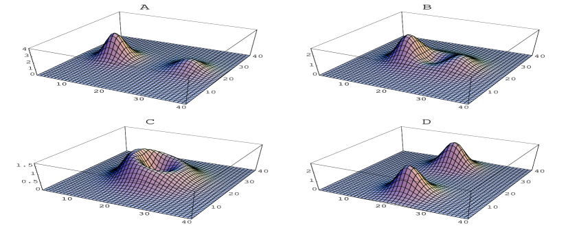
Figure 3: A pair of size $\rho_{1}=6.6$ and $\rho_{2}=8.3$ instantons with perpendicular relative gauge orientations. The centres are separated along the $x_{0}$ axis, the separation, $2|z|$ is 20.0 (A), 13.3 (B), 10.5 (C), and 5.0 (D). The action density is shown in the (01) plane.

This gives rise to a short-to-large distance duality , as long as the relative gauge orientation is not parallel ($\Lambda\neq 0$). The question now arises which of these two descriptions is the “physical” one. To answer this it is again instructive to look at the charge density profile of a set of solutions with varying separations. In fig. 3 we show such a sequence.

The scale parameters, relative orientation and separation, in terms of the l.h.s. of eq. (8), are described by $\lambda_{1}=6.6\sigma_{0}$, $\lambda_{2}=8.3\sigma_{1}$ and $2z=2|z|\sigma_{0}$. For large $|z|$ (A) the constituents are indeed aligned along the 0-axis. As the separation decreases the two lumps merge together into an asymmetric ring (B-C). For even smaller separation (D) the two lumps separate again but now displaced along the 1-axis. Clearly in this case the preferred parametrisation is the r.h.s. of eq. (8), describing two instantons with the same scale parameter $\rho=7.5$, at a distance of 22. Thus, when $|z|^{2}\gg|\Lambda|$, the original description is “physical”, i.e. describing two superposed instantons separated by a distance $2|z|$. When $|z|^{2}\ll|\Lambda|$ it is, however, the dual description which is more “physical”.

Figure 4: The instanton size distribution with the relative orientation being distributed according to the Haar measure. The solid line indicates the distribution of the “physical” (see text) ADHM size parameter, the dotted and the dashed lines are the size distributions determined by the instanton finder algorithms of ref. [8] and ref. [9] respectively.

In fig. 2 we plotted the size distributions obtained when all the pairs were taken oriented parallel in group space. Following the same procedure (including the enhanced tail in the generated size distribution), in fig. 4 we instead consider random colour orientations described by the Haar measure. In this case there is no significant suppression of large instantons. The ambiguity in the physical parametrisation for non-parallel orientation has as a consequence that two instantons can never get closer to each other than $2|z|_{min}\equiv\sqrt{2\rho_{1}\rho_{2}|\sin\varphi|}$, where $\varphi$ is the invariant angle of the relative group orientation. This seems to have no observable effect on the size distribution. Due to the $\sin^{2}\varphi$ factor, the Haar measure very strongly favours (close to) perpendicular orientation, thus our two distributions almost represent the two possible extremes. For the special case of equal size instantons with perpendicular relative orientation one finds at the minimal distance a symmetric ring, also easily described by the conformal ’t Hooft ansatz , by taking $\phi=(x-a)^{-2}+(x-b)^{-2}+(x-c)^{-2}$ with $a,b$ and $c$ forming an equilateral triangle.

We briefly revisit the case of parallel orientations for which the formalism developed in this section is somewhat degenerate. The transition between the two parametrisations (eq. (8)) for $\varphi\approx 0$ occurs at very small separation. In the limit of parallel orientation, one finds

$$\left(y,\,z,\,\rho_{1}\sigma_{0},\,\rho_{2}\sigma_{0},\,0\right)\;\;\longrightarrow\;\;\left(y,\,0,\,\frac{\rho_{1}+\rho_{2}}{\sqrt{2}}\sigma_{0},\,\frac{\rho_{1}-\rho_{2}}{\sqrt{2}}\sigma_{0},\,z\right).$$ (9)

For $z=0$ the two descriptions are equivalent, and there is no way to distinguish between them. One sees that two instantons of scale parameters $\rho_{1,2}$ on top of each other is equivalent to a small instanton of size $\hat{\rho}_{1}=|\rho_{2}-\rho_{1}|/\sqrt{2}$ on top of a larger one of size $\hat{\rho}_{2}=(\rho_{2}+\rho_{1})/\sqrt{2}$. This is consistent with our findings in the previous section for $\rho_{1}=\rho_{2}$, but it should be noted that for $\varphi=0$ any choice of instanton sizes $\hat{\rho}_{1,2}$ are equivalent, provided $\hat{\rho}_{1}^{2}+\hat{\rho}_{2}^{2}=\rho_{1}^{2}+\rho_{2}^{2}$. Only looking at the action distribution, see fig. 1 and the discussion in the previous section, tells us what is the “physical” choice.

4 Conclusions

We have seen how the identification of single instanton parameters becomes ambiguous when instantons overlap. We discussed what happens in the two cases of parallel and random orientation in group space. We expect that the exact way this affects the instanton size distributions measured on the lattice will depend on the relative orientation of nearest neighbour pairs.

To summarise, for non-dilute instanton ensembles the next approximation to a simple superposition is to treat nearest pairs of like charge exactly. Staying as close a possible to the dilute picture one is left with two dual sets of parameters describing the same charge 2 instanton solution. It implies the existence of a minimal distance between the two instantons, which is maximal in the case of perpendicular orientation. In the other extreme case of (nearly) parallel orientation, two close large instantons are more naturally described by a small instanton sitting on top of a large instanton. Thereby one tends to miss large instantons or to underestimate instanton sizes, as was confirmed by a numerical study.

References

References

- [1] T. Schäfer and E.V. Shuryak, Rev. Mod. Phys. 70, 323 (1998).
- [2] D.I. Diakonov, V.Yu. Petrov and P.V. Pobylitsa, Phys. Lett. B 226, 372 (1989); D. Diakonov and V. Petrov, “Confinement from Instantons?”, in: Non-perturbative approaches to Quantum Chromodynamics, Proceedings of the ECT∗ workshop, Trento, July 10-29, 1995, ed. D. Diakonov, Gatchina, 1995, p. 239; T. DeGrand, A. Hasenfratz and T.G. Kovács, Phys. Lett. B 420, 97 (1998); M. Fukushima, H. Suganuma and H. Toki, Phys. Rev. D D60, 094504 (1999); R.C. Brower, D. Chen, J.W. Negele and E. Shuryak, Nucl. Phys. B(Proc. Suppl.) 73, 512 (1999).
-
[3]
P. van Baal, Nucl. Phys. B(Proc. Suppl.) 63A-C, 126 (1998)
(hep-lat/9709066). - [4] T.C. Kraan and P. van Baal, Phys. Lett. B 428, 268 (1998); Nucl. Phys. B 533, 627 (1998); Phys. Lett. B 435, 389 (1998).
- [5] S.J. Jaimungal and A.R. Zhitnitsky, “Coulomb Gas Representation of the QCD Effective Lagrangian”, hep-ph/9905540.
- [6] V. Fateev, I. Frolov and A. Schwartz, Nucl. Phys. B 146, 1 (1979); B. Berg and M. Lüscher, Comm. Math. Phys. 69, 57 (1979); D. Diakonov and M. Maul, Nucl. Phys. B 571, 91 (2000).
- [7] C. Michael and P.S. Spencer, Phys. Rev. D 52, 4691 (1995); D.A. Smith and M.J. Teper, Phys. Rev. D 58, 014505 (1998).
- [8] Ph. de Forcrand, M. García Pérez and I.-O. Stamatescu, Nucl. Phys. B 499, 409 (1997).
- [9] T. DeGrand, A. Hasenfratz and T.G. Kovács, Nucl. Phys. B 505, 417 (1997).
- [10] E.V. Shuryak, “Probing the boundary of the nonperturbative QCD by small size instantons”, hep-ph/9909458; A.E. Drokhov, S.V. Esaibegian, A.E. Maximov and S.V. Mikhailov, Eur. Phys. J. C 13, 331 (2000); G. Münster and Ch. Kamp, “Distribution of instanton sizes in a simplified instanton gas model”, hep-th/0005084.
- [11] M. García Pérez, T.G. Kovács and P. van Baal, Phys. Lett. B 472, 295 (2000) (hep-ph/9911485).
- [12] R. Jackiw, C. Nohl, and C. Rebbi, Phys. Rev. D 15, 1642 (1977).
- [13] S. Donaldson and P. Kronheimer, The Geometry of Four-Manifolds (Oxford University Press, 1990).
- [14] R. Hartshorne, Comm. Math. Phys. 59, 1 (1978); M.F. Atiyah and N.S. Manton, Comm. Math. Phys. 153, 391 (1993).
- [15] M.F. Atiyah, N.J. Hitchin, V. Drinfeld and Yu.I. Manin, Phys. Lett. A 65, 185 (1978).
- [16] N.H. Christ, E.J. Weinberg and N.K. Stanton, Phys. Rev. D 18, 2013 (1978).
- [17] E.F. Corrigan, D.B. Fairlie, S. Templeton and P. Goddard, Nucl. Phys. B 140, 31 (1978).
- [18] H. Osborn, Nucl. Phys. B 159, 497 (1979).
- [19] N. Dorey, V.V. Khoze and M.P. Mattis, Phys. Rev. D 54, 2921 (1996), (Appendix D).
- [20] A.V. Yung, Nucl. Phys. B 297, 47 (1988).