hep-ph/0006154 INLO-PUB 04/00
May 2000

NNLO Evolution of Deep-Inelastic
Structure Functions: the Singlet Case
W.L. van Neerven and A. Vogt
Instituut-Lorentz, University of Leiden
P.O. Box 9506, 2300 RA Leiden, The Netherlands

Abstract

We study the next-to-next-to-leading order (NNLO) evolution of flavour singlet parton densities and structure functions in massless perturbative QCD. Present information on the corresponding three-loop splitting functions is used to derive parametrizations of these quantities, including Bjorken-$x$ dependent estimates of their residual uncertainties. Compact expressions are also provided for the exactly known, but in part rather lengthy two-loop singlet coefficient functions. The size of the NNLO corrections and their effect on the stability under variations of the renormalization and mass-factorizations scales are investigated. Except for rather low values of the scales, the residual uncertainty of the three-loop splitting functions does not lead to relevant effects for $x>10^{-3}$. Inclusion of the NNLO contributions considerably reduces the theoretical uncertainty of determinations of the quark and gluon densities from deep-inelastic structure functions.

PACS: 12.38.Bx, 13.60.Hb

Keywords: Deep-inelastic lepton-hadron scattering; Structure functions; Parton densities; Higher-order QCD corrections

1 Introduction

Structure functions in deep-inelastic scattering (DIS) form the backbone of our knowledge of the proton’s parton densities — which are indispensable for analyses of hard scattering processes at proton–(anti-)proton colliders like Tevatron and the future LHC — and are among the quantities best suited for measuring the strong coupling constant $\alpha_{s}$. The full realization of this potential, however, requires transcending the standard next-to-leading order (NLO) approximation of perturbative QCD summarized in ref. [1]. In fact, the next-to-next-to-leading order (NNLO) subprocess cross-sections (‘coefficient functions’) for DIS have been calculated some time ago [2, 3] (see also refs. [4] for the related Drell-Yan process), but the corresponding three-loop splitting functions governing the NNLO scale dependence (‘evolution’) of the parton densities have not been completed so far (see ref. [5] for an up-to-date progress report).

In a previous paper [6] we have studied the flavour non-singlet sector of the DIS structure functions. It turned out that the available incomplete information on the non-singlet splitting functions [7, 8, 9, 10] facilitates the derivation of approximate expressions which are sufficiently accurate over a rather wide region of parton momenta and the Bjorken variable $x$. In the present paper, we complement those results by corresponding effective parametrizations for the flavour-singlet sector based on the partial information of refs. [8, 11, 12, 13], thus paving the way for promoting, even though only at $x\!>\!10^{-3}$, global analyses [14, 15, 16] of DIS and related processes [4] to NNLO accuracy.

This paper is built up as follows: In Sect. 2 we set up our notations by recalling the general framework for the evolution of singlet parton densities and structure functions in massless perturbative QCD. The expansions of the corresponding splitting functions and coefficient functions are written down up to order $\alpha_{s}^{3}$ for arbitrary values of the renormalization and mass-factorization scales. In Sect. 3 we present compact, but very accurate parametrizations of the exactly known [17, 2, 3], but partly rather lengthy expressions for the two-loop singlet coefficient functions. In Sect. 4 the available constraints [8, 11, 12, 13] on the three-loop singlet splitting functions are utilized for constructing approximate expressions for the $x$-dependence of these functions, including quantitative estimates of the remaining uncertainties. In Sect. 5 we assemble all these results and quantify the impact of the NNLO contributions on the evolution of the singlet quark and gluon densities and on the most important singlet structure function, $F_{2}$. We address the range of applicability of the present approximate results and the improvement of the theoretical accuracy of determinations of the parton densities at NNLO. Finally our results are summarized in Sect. 6. Mellin-$N$ space expressions for our parametrizations of the two-loop coefficient functions of Sect. 3 can be found in the appendix.

2 General Framework

We start by outlining the general formalism for the NNLO evolution of flavour-singlet parton densities and structure functions. The singlet quark density of a hadron is given by

$$\Sigma(x,\mu_{f}^{2},\mu_{r}^{2})\>=\>\sum_{i=1}^{N_{f}}\left[q_{i}(x,\mu_{f}^{2},\mu_{r}^{2})+\bar{q}_{i}(x,\mu_{f}^{2},\mu_{r}^{2})\right]\>\>.$$ (2.1)

Here $q_{i}(x,\mu_{f}^{2},\mu_{r}^{2})$ and $\bar{q}_{i}(x,\mu_{f}^{2},\mu_{r}^{2})$ represent the number distributions of quarks and antiquarks, respectively, in the fractional hadron momentum $x$. The corresponding gluon distribution is denoted by $g(x,\mu_{f}^{2},\mu_{r}^{2})$. The subscript $i$ indicates the flavour of the (anti-) quarks, and $N_{f}$ stands for the number of effectively massless flavours. Finally $\mu_{r}$ and $\mu_{f}$ represent the renormalization and mass-factorization scales, respectively. The singlet quark density (2.1) and the gluon density are constrained by the energy-momentum sum rule

$$\int_{0}^{1}\!dx\>x\left[\Sigma(x,\mu_{f}^{2},\mu_{r}^{2})+g(x,\mu_{f}^{2},\mu_{r}^{2}))\right]\>=\>1\>\>.$$ (2.2)

The scale dependence of the singlet parton densities is given by the evolution equations

$$\frac{d\mbox{\boldmath$q$}}{d\ln\mu_{f}^{2}}\>\equiv\>\frac{d}{d\ln\mu_{f}^{2}}\left(\begin{array}[]{c}\!\Sigma\!\\ g\end{array}\right)\>=\>\left(\begin{array}[]{cc}{\cal P}_{qq}&{\cal P}_{qg}\\ {\cal P}_{gq}&{\cal P}_{gg}\end{array}\right)\otimes\left(\begin{array}[]{c}\!\Sigma\!\\ g\end{array}\right)\>\equiv\>\mbox{\boldmath$P$}\otimes\mbox{\boldmath$q$}\>\>,$$ (2.3)

where $\otimes$ stands for the Mellin convolution in the momentum variable,

$$[a\otimes b](x)\>\equiv\>\int_{x}^{1}\!\frac{dy}{y}\>a(y)\,b\bigg{(}\frac{x}{y}\bigg{)}\>\>.$$ (2.4)

As in some other equations below, the dependence on $x$, $\mu_{f}$ and $\mu_{r}$ has been suppressed in Eq. (2.3). The splitting function ${\cal P}_{qq}$ can be expressed as

$${\cal P}_{qq}\>=\>{\cal P}_{\rm NS}^{+}+{\cal P}_{\rm PS}$$ (2.5)

with

$${\cal P}_{\rm PS}^{\,}\>=\>N_{f}\,({\cal P}_{qq}^{S}+{\cal P}_{\bar{q}q}^{S})\>\>.$$ (2.6)

Here ${\cal P}_{\rm NS}^{+}$ is the non-singlet splitting function discussed up to NNLO in ref. [6], and the ${\cal O}(\alpha_{s}^{2})$ quantities ${\cal P}_{qq}^{S}$ and ${\cal P}_{\bar{q}q}^{S}$ are the flavour independent (‘sea’) contributions to the quark-quark and quark-antiquark splitting functions ${\cal P}_{q_{i}q_{k}}$ and ${\cal P}_{\bar{q}_{i}q_{k}}$, respectively. The non-singlet contribution dominates Eq. (2.5) at large $x$, where the pure singlet term ${\cal P}_{\rm PS}^{\,}$ is very small. At small $x$, on the other hand, the latter contribution takes over as $x{\cal P}_{\rm PS}^{\,}$, unlike $x{\cal P}_{\rm NS}^{+}$, does not vanish for $x\!\rightarrow\!0$. The gluon-quark and quark-gluon entries in (2.3) are given by

$${\cal P}_{qg}\>=\>N_{f}\,{\cal P}_{q_{i}g}\>\>,\quad{\cal P}_{gq}\>=\>{\cal P}_{gq_{i}}$$ (2.7)

in terms of the flavour-independent splitting functions ${\cal P}_{q_{i}g}={\cal P}_{\bar{q}_{i}g}$ and ${\cal P}_{gq_{i}}={\cal P}_{g\bar{q}_{i}}$. With the exception of the lowest-order approximation to ${\cal P}_{qg}$, neither of the quantities $x{\cal P}_{qg}$, $x{\cal P}_{gq}$ and $x{\cal P}_{gg}$ vanishes for $x\!\rightarrow\!0$.

The NNLO expansion of the splitting-function matrix $P$ in Eq. (2.3) reads

$$\mbox{\boldmath$P$}\Big{(}x,\alpha_{s}(\mu_{r}^{2}),L_{R}\Big{)} \!=\!\! \quad a_{s}\,\mbox{\boldmath$P$}^{(0)}(x)$$

$$\mbox{}\!\!+a_{s}^{2}\,\Big{(}\mbox{\boldmath$P$}^{(1)}(x)-\beta_{0}L_{R}\mbox{\boldmath$P$}^{(0)}(x)\Big{)}\>$$

$$\mbox{}\!\!+a_{s}^{3}\,\Big{(}\mbox{\boldmath$P$}^{(2)}(x)-2\beta_{0}L_{R}\mbox{\boldmath$P$}^{(1)}(x)-\Big{\{}\beta_{1}L_{R}-\beta_{0}^{2}L_{R}^{2}\Big{\}}\mbox{\boldmath$P$}^{(0)}(x)\Big{)}+\ldots\>\>.$$

In Eq. (2.8) and in what follows we use the abbreviations

$$a_{s}\>\equiv\>\frac{\alpha_{s}(\mu_{r}^{2})}{4\pi}$$ (2.9)

for the running coupling, and

$$L_{M}\>\equiv\>\ln\frac{Q^{2}}{\mu_{f}^{2}}\>\>,\quad L_{R}\>\equiv\>\ln\frac{\mu_{f}^{2}}{\mu_{r}^{2}}$$ (2.10)

for the scale logarithms. The one- and two-loop matrices $\mbox{\boldmath$P$}^{(0)}(x)$ and $\mbox{\boldmath$P$}^{(1)}(x)$ in Eq. (2.8) are known for a long time [1], see also ref. [18] for the solution of an earlier problem in the covariant-gauge calculation of $P_{gg}^{(1)}$. The three-loop quantities $P_{ij}^{(2)}(x)$ are the subject of Sect. 4. The consistency of the evolution equations (2.3) with the momentum sum rule (2.2) imposes the following constraints on the second moments of $P_{ij}^{(l)}(x)\,$:

$$P_{qq}^{(l)}(N)+P_{gq}^{(l)}(N) = 0$$

$$P_{qg}^{(l)}(N)+P_{gg}^{(l)}(N) = 0\quad\mbox{for}\quad N=2\>\>,$$ (2.11)

where

$$a(N)\>\equiv\>\int_{0}^{1}\!dx\,x^{N-1}a(x)\>\>.$$ (2.12)

The constants $\beta_{i}$ in Eq. (2.8) represent the perturbative coefficients of the QCD $\beta$-function

$$\frac{da_{s}}{d\ln\mu_{r}^{2}}\>=\>\beta(a_{s})\>=\>-\sum_{l=0}a_{s}^{l+2}\beta_{l}\>\>.$$ (2.13)

The coefficients $\beta_{0},\,\beta_{1}$ and $\beta_{2}$ required for NNLO calculations can be found in refs. [1] and [19], respectively. Finally the $L_{R}$ terms in Eq. (2.8) are obtained from the expression for $\mu_{r}=\mu_{f}$ by inserting the expansion of $a_{s}(\mu_{f}^{2})$ in terms of $a_{s}(\mu_{r}^{2})$,

$$a_{s}(\mu_{f}^{2})=a_{s}(\mu_{r}^{2})-\beta_{0}L_{R}\,a_{s}^{2}(\mu_{r}^{2})-\left\{\beta_{1}L_{R}-\beta_{0}^{2}L_{R}^{2}\right\}a_{s}^{3}(\mu_{r}^{2})+\ldots\>\>.$$ (2.14)

The singlet structure functions $F_{a,S}$, $a=1,\,2$, are in Bjorken-$x$ space obtained by the convolution (2.4) of the solution of Eq. (2.3) with the corresponding coefficient functions,

$$\eta_{a}F_{a,\rm S}(x,Q^{2}) \!=\! \left[{\cal C}_{a,q}(a_{s},L_{M},L_{R})\otimes\Sigma(\mu_{f}^{2},\mu_{r}^{2})+{\cal C}_{a,g}(a_{s},L_{M},L_{R})\otimes g(\mu_{f}^{2},\mu_{r}^{2})\right](x)\quad$$ (2.15)

$$\!\equiv\! \left[\mbox{\boldmath$C$}_{a}(a_{s},L_{M},L_{R})\otimes\mbox{\boldmath$q$}(\mu_{f}^{2},\mu_{r}^{2})\right](x)\>\>.$$

Here the electroweak charge factor is included in $\eta_{a}$, e.g., $\eta_{1}=2\,\langle e^{2}\rangle^{-1}$ and $\eta_{2}=(x\,\langle e^{2}\rangle)^{-1}$ for electromagnetic scattering, with an average squared charge $\langle e^{2}\rangle=5/18$ for an even $N_{f}$. Up to third order in $\alpha_{s}$ the expansion of the coefficient functions takes the form

$$\mbox{\boldmath$C$}_{a}(x,\alpha_{s}(\mu_{r}^{2}),L_{M},L_{R}) = \mbox{\boldmath$C$}_{a}^{(0)}(x)\,+\,a_{s}\mbox{\boldmath$C$}_{a}^{(1)}(x,L_{M})\,+$$

$$\mbox{}a_{s}^{2}\mbox{\boldmath$C$}_{a}^{(2)}(x,L_{M},L_{R})\,+\,a_{s}^{3}\mbox{\boldmath$C$}_{a}^{(3)}(x,L_{M},L_{R})\,+\,\ldots\quad$$

$$\!\!\stackrel{{\scriptstyle{\mu_{r}=\mu_{f}}}}{{=}}\!\! \mbox{\boldmath$c$}_{a}^{(0)}(x)\,+\,\sum_{l=1}^{3}a_{s}^{l}\left(\mbox{\boldmath$c$}_{a}^{(l)}(x)+\sum_{m=1}^{l}\mbox{\boldmath$c$}_{a}^{(l,m)}(x)L_{M}^{m}\right)\,+\,\ldots\>\>,\quad$$

where $\mbox{\boldmath$c$}_{a}^{(0)}(x)\equiv(\,c_{a,q}^{(0)}(x)\,,\,c_{a,g}^{(0)}(x)\,)=(\,\delta(1-x)\,,\,0\,)$ represents the parton-model result. The first-order corrections $\mbox{\boldmath$c$}_{a}^{(1)}(x)$ can be found in ref. [1]; the two-loop coefficient functions $c_{a,q}^{(2)}(x)$ and $c_{a,g}^{(2)}(x)$ computed in refs. [2, 3] are briefly addressed in Sect. 3. The terms up to order $\alpha_{s}^{2}$ in Eq. (2.16) contribute to $F_{a}$ in the NNLO approximation. The $\alpha_{s}^{3}$ terms only enter for $dF_{a}/d\ln Q^{2}$, hence the scale-independent three-loop quantities $\mbox{\boldmath$c$}_{a}^{(3)}(x)$ are not needed here. The coefficients $\mbox{\boldmath$c$}_{a}^{(l,m)}(x)$ in the second part of Eq. (2.16) can be conveniently written in a recursive manner as

$$\mbox{\boldmath$c$}_{a}^{(1,1)} \!=\! \mbox{\boldmath$c$}_{a}^{(0)}\otimes\mbox{\boldmath$P$}^{(0)}$$

$$\mbox{\boldmath$c$}_{a}^{(2,1)} \!=\! \mbox{\boldmath$c$}_{a}^{(0)}\otimes\mbox{\boldmath$P$}^{(1)}+\mbox{\boldmath$c$}_{a}^{(1)}\otimes(\mbox{\boldmath$P$}^{(0)}-\beta_{0}\mbox{\boldmath$1$})$$

$$\mbox{\boldmath$c$}_{a}^{(2,2)} \!=\! \frac{1}{2}\mbox{\boldmath$c$}_{a}^{(1,1)}\otimes(\mbox{\boldmath$P$}^{(0)}-\beta_{0}\mbox{\boldmath$1$})$$

$$\mbox{\boldmath$c$}_{a}^{(3,1)} \!=\! \mbox{\boldmath$c$}_{a}^{(0)}\otimes\mbox{\boldmath$P$}^{(2)}+\mbox{\boldmath$c$}_{a}^{(1)}\otimes(\mbox{\boldmath$P$}^{(1)}-\beta_{1}\mbox{\boldmath$1$})+\mbox{\boldmath$c$}_{a}^{(2)}\otimes(\mbox{\boldmath$P$}^{(0)}-2\beta_{0}\mbox{\boldmath$1$})$$

$$\mbox{\boldmath$c$}_{a}^{(3,2)} \!=\! \frac{1}{2}\bigg{\{}\mbox{\boldmath$c$}_{a}^{(1,1)}\otimes(\mbox{\boldmath$P$}^{(1)}-\beta_{1}\mbox{\boldmath$1$})+\mbox{\boldmath$c$}_{a}^{(2,1)}\otimes(\mbox{\boldmath$P$}^{(0)}-2\beta_{0}\mbox{\boldmath$1$})\bigg{\}}$$

$$\mbox{\boldmath$c$}_{a}^{(3,3)} \!=\! \frac{1}{3}\mbox{\boldmath$c$}_{a}^{(2,2)}\otimes(\mbox{\boldmath$P$}^{(0)}-2\beta_{0}\mbox{\boldmath$1$})\>\>.$$ (2.17)

Eqs. (2.17) can be derived by identifying the results of the following two calculations of $dF_{a,S}/d\ln Q^{2}$ at $\mu_{r}^{2}=\mu_{f}^{2}=Q^{2}$: (a) with the scales identified in the beginning (using Eqs. (2.3) and (2.13), and (b) with the scales set equal only at the end (after differentiating the logarithms in Eq. (2.16) ). Finally the coefficients $\mbox{\boldmath$C$}_{a}^{(2)}$ and $\mbox{\boldmath$C$}_{a}^{(3)}$ for $\mu_{f}\neq\mu_{r}$ in Eq. (2.16) are obtained from these results by Eq. (2.14):

$$\mbox{\boldmath$C$}_{a}^{(2)}(x,L_{M},L_{R}) \!=\! \mbox{\boldmath$C$}_{a}^{(2)}(x,L_{M},0)-\beta_{0}L_{r}\,\mbox{\boldmath$C$}_{a}^{(1)}(x,L_{M})$$

$$\mbox{\boldmath$C$}_{a}^{(3)}(x,L_{M},L_{R}) \!=\! \mbox{\boldmath$C$}_{a}^{(3)}(x,L_{M},0)-2\beta_{0}L_{r}\,\mbox{\boldmath$C$}_{a}^{(2)}(x,L_{M},0)$$

$$\mbox{}-\left\{\beta_{1}L_{R}-\beta_{0}^{2}L_{R}^{2}\right\}\mbox{\boldmath$C$}_{a}^{(1)}(x,L_{M})\>\>.$$

The above-mentioned calculations of $\beta_{2}$ [19] and $\mbox{\boldmath$c$}_{a}^{(2)}(x)$ [2, 3] have been performed in the $\overline{\mbox{MS}}$ renormalization and factorization schemes. The other factorization scheme widely used in NLO analyses of unpolarized deep-inelastic scattering is the so-called DIS scheme. In this scheme the expression for $F_{2,S}$ is reduced, for the choice $\mu_{r}^{2}=\mu_{f}^{2}=Q^{2}$ adopted for the rest of this section, to its parton-model form $\eta_{2\,}F_{2,S}(x,Q^{2})=\widetilde{\Sigma}(x,Q^{2})$, i.e.,

$$\widetilde{c}_{2,q}^{\,(l)}(x)\>\equiv\>\widetilde{c}_{2,g}^{\,(l)}(x)\>=\>0\quad\mbox{for}\quad l\geq 1\>\>.$$ (2.19)

Here and in the following DIS-scheme quantities are marked by a tilde. The corresponding singlet parton densities can be defined by

$$\widetilde{\mbox{\boldmath$q$}}\>\equiv\>\left(\begin{array}[]{c}\!\widetilde{\Sigma}\!\\ \widetilde{g}\end{array}\right)\>=\>\left(\begin{array}[]{rr}c_{2,q}&c_{2,g}\\ -c_{2,q}&-c_{2,g}\end{array}\right)\otimes\left(\begin{array}[]{c}\!\Sigma\!\\ g\end{array}\right)\>\equiv\>\mbox{\boldmath$Z$}\otimes\mbox{\boldmath$q$}\>\>.$$ (2.20)

The upper row of the transformation matrix $Z$ is fixed by Eq. (2.19). The lower row is constrained only by the momentum sum rule (2.2) which fixes its form for the second moment, $N=2$. The extension of this constraint to all $N$,

$$\tilde{\Sigma}(N)+\tilde{g}(N)\>=\>\Sigma(N)+g(N)\>\>,$$ (2.21)

in Eq. (2.20) is the obvious generalization of the standard NLO convention of ref. [20] to all orders. The DIS-scheme splitting functions for $\mu_{r}^{2}=\mu_{f}^{2}=Q^{2}$ can be expressed in terms of their $\overline{\mbox{MS}}$ counterparts by differentiating of Eq. (2.20) with respect to $Q^{2}$:

$$\widetilde{\mbox{\boldmath$P$}}\>=\>\left(\mbox{\boldmath$Z$}\otimes\mbox{\boldmath$P$}+\beta\,\frac{d\mbox{\boldmath$Z$}}{da_{s}}\right)\otimes\mbox{\boldmath$Z$}^{-1}\>\>.$$ (2.22)

Insertion of the expansions (2.8) for $L_{R}=0$, (2.13) and

$$\mbox{\boldmath$Z$}(x,a_{s})\>=\>\mbox{\boldmath$1$}+\sum_{l=1}a_{s}^{l}\mbox{\boldmath$Z$}^{(l)}(x)\>=\>\mbox{\boldmath$1$}+\sum_{l=1}a_{s}^{l}\left(\begin{array}[]{rr}c_{2,q}^{(l)}(x)&c_{2,g}^{(l)}(x)\\[2.84526pt] -c_{2,q}^{(l)}(x)&-c_{2,g}^{(l)}(x)\end{array}\right)$$ (2.23)

then yields

$$\widetilde{\mbox{\boldmath$P$}} \!=\! \quad\>a_{s}\mbox{\boldmath$P$}_{0}$$

$$\mbox{}+a_{s}^{2}\left(\mbox{\boldmath$P$}^{(1)}+[\mbox{\boldmath$Z$}^{(1)},\mbox{\boldmath$P$}^{(0)}]-\beta_{0}\mbox{\boldmath$Z$}^{(1)}\right)$$

$$\mbox{}+a_{s}^{3}\left(\mbox{\boldmath$P$}^{(2)}+[\mbox{\boldmath$Z$}^{(2)},\mbox{\boldmath$P$}^{(0)}]+[\mbox{\boldmath$Z$}^{(1)},\mbox{\boldmath$P$}^{(1)}]-[\mbox{\boldmath$Z$}^{(1)},\mbox{\boldmath$P$}^{(0)}]\otimes\mbox{\boldmath$Z$}^{(1)}\right.$$

$$\mbox{}\quad\quad+\left.\beta_{0}\mbox{\boldmath$Z$}^{(1)}\otimes\mbox{\boldmath$Z$}^{(1)}-2\beta_{0}\mbox{\boldmath$Z$}^{(2)}-\beta_{1}\mbox{\boldmath$Z$}^{(1)}\right)\>+\>\ldots\>\>,$$

where

$$[\mbox{\boldmath$Z$}^{(l)},\mbox{\boldmath$P$}^{(m)}]\equiv\mbox{\boldmath$Z$}^{(l)}\otimes\mbox{\boldmath$P$}^{(m)}-\mbox{\boldmath$P$}^{(m)}\otimes\mbox{\boldmath$Z$}^{(l)}\>\>.$$ (2.25)

The coefficient functions and splitting functions for $\mu_{r}^{2}\neq\mu_{f}^{2}\neq Q^{2}$ can by obtained from Eqs. (2.19) and (2.24) using Eqs. (2.16)–(2.18) and (2.8), respectively. In the present article Eq. (2.24) will be only employed in Sect. 4 for transforming a small-$x$ constraint obtained for $\widetilde{P}_{gg}^{(2)}$ [12] into the $\overline{\mbox{MS}}$ scheme adopted for the rest of this paper.

3 The 2-loop singlet coefficient functions

Beyond the first order, $l=1$, the exact expressions for the scale independent parts $\mbox{\boldmath$c$}_{a}^{(l)}(x)$ of the coefficient functions (2.16) are rather lengthy and involve higher transcendental functions. Moreover, the convolutions entering the expressions (2.17) for $\mu_{f}^{2}\neq Q^{2}$ (given explicitly for $l=2$ in ref. [3]) and the factorization scheme transformation (2.24) become increasingly cumbersome at higher orders. The latter complications can be circumvented by using the moment-space technique [20, 22], as the convolution (2.4) reduces to a simple product in $N$-space. This technique, however, requires the analytic continuation of all ingredients to complex values of $N$ in Eq. (2.12), which itself becomes rather involved already for the exact expressions for $\mbox{\boldmath$c$}_{a}^{(2)}(x)$ [23]. Hence it is convenient, for both $x$-space and $N$-space applications, to dispose of compact parametrizations of these quantities.

For the non-singlet components $c_{L,\rm NS}^{(2)}(x)$ [17] and $c_{2,\rm NS}^{(2)}(x)$ [2] of

$$c_{a,q}^{(2)}(x)\>=\>c_{a,{\rm NS}}^{(2)}(x)+c_{a,{\rm PS}}^{(2)}(x)\>\>,$$ (3.1)

where $F_{L}\equiv F_{2}-2xF_{1}$, such parametrizations have been given in ref. [6] in terms of

$$L_{0}\>\equiv\>\ln x\>\>,\quad L_{1}\>\equiv\>\ln(1-x)$$ (3.2)

and simpler functions of $x$. The pure singlet pieces in Eq. (3.1) can be approximated by

$$c_{L,{\rm PS}}^{(2)}(x) = N_{f}\>\Big{\{}(15.94-5.212\,x)(1-x)^{2}L_{1}+(0.421+1.520\,x)L_{0}^{2}$$ (3.3)

$$\mbox{}+28.09\,(1-x)L_{0}-(2.370\,x^{-1}-19.27)(1-x)^{3}\Big{\}}\>\>,$$

$$c_{2,{\rm PS}}^{(2)}(x) = N_{f}\>\Big{\{}-0.101\,(1-x)L_{1}^{3}-(24.75-13.80\,x)L_{1}L_{0}^{2}+30.23L_{1}L_{0}$$ (3.4)

$$\mbox{}+4.310\,L_{0}^{3}-2.086\,L_{0}^{2}+39.78\,L_{0}+5.290(x^{-1}-1)\Big{\}}\>\>.$$

The corresponding gluon coefficient functions [2] can be parametrized as

$$c_{L,g}^{(2)}(x) = N_{f}\>\Big{\{}(94.74-49.20\,x)(1-x)L_{1}^{2}+864.8\,(1-x)L_{1}+1161\,xL_{1}L_{0}$$ (3.5)

$$\mbox{}+60.06\,xL_{0}^{2}+39.66\,(1-x)L_{0}-5.333\,(x^{-1}-1)\Big{\}}\>\>,$$

$$c_{2,g}^{(2)}(x) = N_{f}\>\Big{\{}(6.445+209.4\,(1-x))L_{1}^{3}-24.00\,L_{1}^{2}+(1494\,x^{-1}-1483)L_{1}$$ (3.6)

$$\mbox{}+L_{1}L_{0}(-871.8\,L_{1}-724.1L_{0})+5.319L_{0}^{3}-59.48\,L_{0}^{2}-284.8\,L_{0}$$

$$\mbox{}+11.90\,x^{-1}+392.4-0.28\,\delta(1-x)\Big{\}}\>\>.$$

Note the small $\delta(1-x)$ term in the parametrization of $c_{2,g}^{(2)}$, which is of course absent in the exact expression, but useful for obtaining high-accuracy convolutions here. The parametrizations (3.3)–(3.6) deviate from the exact results by no more than a few permille.

4 The 3-loop singlet splitting functions

Only partial results have been obtained so far for the $O(\alpha_{s}^{3})$ terms $P_{ij}^{(2)}(x)$ of the singlet splitting functions (2.8). As the full $x$-dependence is known just for the $C_{A}N_{f}^{2}$ part of $P_{gg}^{(2)}$ [13], the backbone of the available constraints are the lowest four even-integer moments (2.12) of these terms,

$$P_{ij}^{(2)}(N)\quad\mbox{for}\quad N\>=\>2,\,4,\,6,\,8\>\>,$$ (4.1)

calculated in ref. [8]. This is one moment less than determined for the non-singlet quantity $P_{\rm NS}^{(2)+}(x)$ [7, 8], due to the greater technical complexity of the singlet computation.

The $1/[1-x]_{+}$ soft-gluon contributions to the gluon-gluon splitting functions $P_{gg}^{(0)}$ and $P_{gg}^{(1)}$ are related to their quark-quark counterparts by

$$(1-x)P_{gg}^{(l)}(x)\bigg{|}_{x=1}\>=\>\frac{C_{A}}{C_{F}}\>(1-x)P_{qq}^{(l)}(x)\bigg{|}_{x=1}\>=\>\frac{C_{A}}{C_{F}}\>(1-x)P_{\rm NS}^{(l)}(x)\bigg{|}_{x=1}$$ (4.2)

(${\cal P}_{\rm PS}^{\,}$ in Eq. (2.5) vanishes at $x=1$). This relation also applies to the leading-$N_{f}$ terms [9, 13] of $P_{gg}^{(2)}$ and $P_{\rm NS}^{(2)}$. We will assume that Eq. (4.2) holds generally for $l=2$.

The small-$x$ behaviour of $P_{ij}^{(2)}(x)$ is not constrained by Eq. (4.1). The leading $x\!\rightarrow\!0$ terms $\propto\frac{1}{x}\ln x$ have been determined from small-$x$ resummations, however, for $P_{qq}^{(2)}$, $P_{qg}^{(2)}$ and $P_{gg}^{(2)}$. Specifically, the gluon-quark and quark-quark entries read [11]

$$P_{qg,x\rightarrow 0}^{(2)} = \mbox{}\!\!-\frac{896}{27}\>C_{A}^{2}N_{f}\>\frac{\ln x}{x}\>+\>O\left(\frac{1}{x}\right)\>\>,$$ (4.3)

$$P_{qq,x\rightarrow 0}^{(2)} = \quad\frac{C_{F}}{C_{A}}\>P_{qg,x\rightarrow 0}^{(2)}\>\>+\>O\left(\frac{1}{x}\right)\>\>.$$ (4.4)

The corresponding gluon-gluon result can be inferred [24] from the larger eigenvalue of $\mbox{\boldmath$P$}_{x\rightarrow 0}^{(2)}$ completed in ref. [12] in a scheme equivalent to the DIS scheme up to 3-loop order:

$$\widetilde{P}_{gg,x\rightarrow 0}^{(2)}=\left\{6320-864\,\zeta(3)-1584\,\zeta(2)+N_{f}\left(\frac{1136}{3}-96\,\zeta(2)\right)\right\}\frac{\ln x}{x}\>+\>O\left(\frac{1}{x}\right)\>\>,$$ (4.5)

where $\zeta(2)=\pi^{2}/6$ and $\zeta(3)\simeq 1.202057$. For this contribution the scheme transformation (2.24) schemes simplifies to

$$\widetilde{P}_{gg,x\rightarrow 0}^{(2)}\>=\>P_{gg,x\rightarrow 0}^{(2)}-\Big{(}P_{gq}^{(0)}\otimes c_{2,g}^{(2)}\Big{)}_{x\rightarrow 0}\>+\>O\left(\frac{1}{x}\right)\>\>,$$ (4.6)

yielding

$$P_{gg,x\rightarrow 0}^{(2)}\>=\>\left\{6320-864\,\zeta(3)-1584\,\zeta(2)+N_{f}\left(\frac{4720}{27}-\frac{32}{3}\,\zeta(2)\right)\right\}\frac{\ln x}{x}\>+\>O\left(\frac{1}{x}\right)\>\>.$$ (4.7)

Eqs. (4.6) and (4.7) are most easily derived via moment-space, see the appendix.

In the following the above information will be used for approximate representations of

$$P_{ij}^{(2)}(x)\>=\>P_{ij,0}^{(2)}(x)+N_{f}P_{ij,1}^{(2)}(x)+N_{f}^{2}P_{ij,2}^{(2)}(x)\>\>,$$ (4.8)

where the $N_{f}$-independent terms are absent in $P_{\rm PS}^{(2)}$ and $P_{qg}^{(2)}$ according to Eqs. (2.6) and (2.7). For each of the ten remaining contributions $P_{ij,m}^{(2)}$ we employ the ansatz

$$P_{ij,m}^{(2)}(x)\>=\>\sum_{n=1}^{4}A_{n}f_{n}(x)+f_{e}(x)\>\>.$$ (4.9)

Except for the $\delta(1-x)$ terms in $P_{gg,m}^{(2)}$, the basis functions $f_{n}$ are build up of powers of $\ln(1-x)$, $x$, and $\ln x$. Generally we choose the functions $f_{n}$ to include at least one function peaking as $x\!\rightarrow\!1$ (except for $P_{\rm PS}^{(2)}$, of course), one rather flat function (a small non-negative power of $x$), and one function peaking as $x\!\rightarrow\!0$. For each choice of the building blocks $f_{n}$, the coefficients $A_{n}$ are determined from the four linear equations provided by the moments (4.1) of ref. [8] after taking into account the additional information (4.2)–(4.4) and (4.7) collected in the function $f_{e}$ in Eq. (4.9). The residual uncertainty of the functions $P_{ij,m}^{(2)}$ is estimated by varying the choice of the basis functions $f_{n}$. Finally two approximate expressions are selected for each of the six quantities $P_{gq,0\,}^{(2)}$, $P_{gg,0}^{(2)}$ and $P_{ij,1}^{(2)}$ which are representative for the respective present uncertainty band. The $N_{f}^{2}$ pieces $P_{ij,2}^{(2)}$ are smaller in absolute size and uncertainty than those contributions, hence for them it suffices to select just one central representative.

Before proceeding to our approximations of the coefficients $P_{ij,m}^{(2)}$ in Eq. (4.8), it is worthwhile to discuss another constraint on the singlet splitting functions which has served as an important check for the calculations of the NLO quantities $P_{ij}^{(1)}(x)$ in the unpolarized [1] as well as in the polarized case [25, 26]. This is the relation

$$P_{qq,{\rm DR}}^{(l)}(x)+P_{gq,{\rm DR}}^{(l)}(x)-P_{qg,{\rm DR}}^{(l)}(x)-P_{gg,{\rm DR}}^{(l)}(x)\>=\>0$$ (4.10)

for the choice

$$C_{A}\>\equiv\>N_{c}\>=\>C_{F}\>=\>N_{f}$$

of the colour factors leading to a ${\cal N}\!=\!1$ supersymmetric theory. As indicated, Eq. (4.10) holds in the dimensional reduction (DR) scheme respecting the supersymmetry, but not in the usual $\overline{\mbox{MS}}$ scheme based on dimensional regularization. The terms breaking the relation (4.10) in the $\overline{\mbox{MS}}$ scheme for $l=1$ are, however, much simpler than the functions $P_{ij}^{(1)}(x)$ themselves. They involve only $\ln^{1}x$ and powers of $x$, however including the leading small-$x$ term $1/x$ [27]. It should also be noted that Eq. (4.10) does not in all cases introduce a relation between different functions $P_{ij}^{(l)}$. For instance, the leading large-$x$ terms of $P_{gq}^{(1)}$ and $P_{qg}^{(1)}$, $\ln^{2}(1-x)$ and $\ln(1-x)$, cancel already on the level in the individual splitting functions for the choice (4.11), not only after forming the combination (4.10), as can be readily read off from the tables in refs. [28, 29].

The transformation of the splitting functions from the DR to the $\overline{\mbox{MS}}$ scheme is presently unknown for $l=2$ (its derivation would require repeating the calculation of the finite terms of the two-loop operator matrix elements of ref. [31] in the DR scheme). It is expected, however, that the terms breaking Eq. (4.10) in the $\overline{\mbox{MS}}$ scheme at $l=2$ are again comparatively simple and do not include terms like $\ln^{3}(1-x)$, $\ln^{4}(1-x)$, and $\ln^{4}x$. Under this assumption that relation does provide some constraints on the functions $P_{ij}^{(2)}$. In view of their limitations discussed above for the NLO case, however, these few additional constraints do not justify moving from Eq. (4.8) to a complete colour-factor decomposition involving twenty-three instead of ten unknown functions $P_{ij,m}^{(2)}$.

We now illustrate the details of our approximation procedure outlined above for the case of the gluon-quark splitting functions $P_{qg}$ dominating the small-$x$ evolution of the singlet quark density. While the lowest-order result $P_{qg}^{(0)}$ contains no logarithms, terms up to $\ln^{2}(1-x)$ and $\ln^{2}x$ occur in $P_{qg}^{(1)}$. Hence we expect contributions up to $\ln^{4}(1-x)$ and $\ln^{4}x$ in the three-loop splitting function $P_{qg}^{(2)}$ due to the additional loop or emission. Thus a reasonable choice of the trial functions for $P_{qg,1}^{(2)}$ is given by

$$\begin{array}[b]{ccccc}f_{1}(x)&=&\ln^{2}x&\mbox{ or }&\ln^{3}x\\[1.42262pt] f_{2}(x)&=&1&\mbox{ or }&x\\[1.42262pt] f_{3}(x)&=&\ln\,(1-x)&\mbox{ or }&\ln^{2}(1-x)\\[1.42262pt] f_{4}(x)&=&\ln^{3}(1-x)&\mbox{ or }&\ln^{4}(1-x)\\[5.69054pt] f_{e}(x)&=&\lx@intercol{\displaystyle-\frac{896}{27}\,C_{A}^{2}N_{f}\left(\frac{\ln x}{x}+\frac{\lambda}{x}\right)}\hfil\lx@intercol\end{array},\quad\lambda=0\>\mbox{ or }\>4\>\>.$$ (4.11)

As for all other cases in which the $\frac{1}{x}\ln x$ terms are known, we do not include the subleading contribution $1/x$ in the functions $f_{n}$, but vary its coefficient by hand up to a value suggested by the expansion of the moment-space expressions $P_{ij}^{(0)}(N)$ and $P_{ij}^{(0)}(N)$ around $N=1$ [32]. Four of the thirty-two combinations resulting from Eq. (4.12) (those combining $f_{1}=\ln^{2}x$ with $f_{2}=1$ and $\lambda=4$) lead to an almost singular system for the coefficients $A_{n}$ which causes overly large oscillations of the corresponding results for $P_{qg,1}^{(2)}(x)$. The remaining twenty-eight approximations, of which four are selected for further consideration, are displayed in Fig. 1.

Figure 1: Approximations of the $N_{f}^{1}$ part $P_{qg,1}^{(2)}$ of the three-loop splitting function $P_{qg}^{(2)}(x)$ in Eq. (2.8), as obtained from the four moments (4.1) by means of Eqs. (4.9) and (4.12). The full and dashed curves represent the functions selected for further consideration. The upper group of curves in the right plot is for $\lambda=0$ in Eq.(4.12), the lower group for $\lambda=4$.

Figure 2: Left: as Fig. 1, but for the $N_{f}^{2}$ contribution $P_{qg,2}^{(2)}(x)$ using Eqs. (4.9) and (4.13). Right: convolution of the approximations A–D of Fig. 1, combined for $N_{f}=4$ with the result selected for $P_{qg,2}^{(2)}$ in the left part, with a typical gluon density of the proton.

Our corresponding ansatz for the $N_{f}^{2}$ part reads

$$\begin{array}[b]{ccccccc}f_{1}(x)&=&\ln x&\mbox{ or }&\ln^{2}x&\mbox{ or }&\ln^{3}x\\[1.42262pt] f_{2}(x)&=&1&\mbox{ or }&x&&\\[1.42262pt] f_{3}(x)&=&\ln(1-x)&\mbox{ or }&\ln^{2}(1-x)&\mbox{ or }&\ln^{3}(1-x)\\[1.42262pt] f_{4}(x)&=&{\displaystyle\frac{1}{x}}&\mbox{and}&\lx@intercol\hfil f_{e}(x)\>=\>0\>\>.\hfil\lx@intercol&\end{array}$$ (4.12)

Here and for all other $N_{f}^{2}$ terms the $1/x$ contribution is included in the functions $f_{n}$, as no information about its magnitude is available. Fifteen of the eighteen combinations resulting from Eq. (4.13) are shown in the left part of Fig. 2. The three combinations involving $f_{1}=\ln^{3}x$ and $f_{2}=x$ are rejected for the same reason as the four expressions for $P_{qg,1}^{(2)}$ mentioned above.

In the right part of Fig. 2 the approximations selected for $P_{qg,1}^{(2)}$ and $P_{qg,2}^{(2)}$ have been combined into Eq. (4.8) for $N_{f}=4$ and convoluted with a typical example for the gluon density of the proton. Needless to say that it is this combination $P_{qg}^{(2)}\otimes g$ (divided by $g(x)$ for display purposes in Fig. 2) and not $P_{qg}^{(2)}(x)$ itself which enters the evolution equations (2.3) and thus the structure functions (2.15). At moderately large $x$, $0.1\!<\!x\!<\!0.7$, the spread of the convolutions in Fig. 2 is small, typically about 5%, much smaller than that for the splitting function itself, as the convolution (2.4) tends to wash out the oscillating differences of Fig. 1 to a large extent.

The large-$x$ behaviour of the splitting functions is very important also at small $x$, as can be inferred from a comparison of Figs. 1 and 2: while $P_{qg}^{(2)}(x)$ is dominated at $x<10^{-2}$ by the $\frac{1}{x}\ln x$ and $1/x$ terms, this does by no means hold for $[P_{qg}^{(2)}\otimes g](x)$. For instance, the leftmost cross-over of the approximations C ($\lambda\!=\!4$) and D ($\lambda\!=\!0$) for $P_{qg}^{(2)}$ is at $x=0.03$, but the convolution for the function D does not exceed that for the approximation C above $x=10^{-3}$. An even more striking illustration can be obtained by keeping only the small-$x$ function $f_{e}$ in Eq. (4.12) for $P_{ij,1}$. The convolution then yields $(P_{qg}^{(2)}\otimes g)/g\simeq 4000$ and $-6000$ for $\lambda=0$ and $\lambda=4$ at $x=10^{-3}$, respectively, instead of the spread between about 700 and 1300 found after taking into account the large-$x$ constraints (4.1).

Except close to the unavoidable cross-over points, the functions A and B are representative for the uncertainty bands of Figs. 1 and 2. Hence these approximations are chosen as our final results for the gluon-quark splitting function:

$$P^{(2)A}_{{qg},\,1}(x)\! = -19.5515\>L_{1}^{3}+707.438\>L_{1}+2300.986+814.928\>L_{0}^{2}-\frac{896}{3}\>\frac{L_{0}+4}{x}\quad\quad\quad$$

$$P^{(2)B}_{{qg},\,1}(x)\! = 10.8972\>L_{1}^{4}-315.331\>L_{1}^{2}+902.843\>x-1054.09\>L_{0}^{2}-\frac{896}{3}\>\frac{L_{0}}{x}$$ (4.13)

with $L_{0}$ and $L_{1}$ as defined in Eq. (3.2). The selected approximation for the $N_{f}^{2}$ piece reads

$$P^{(2)}_{{qg},\,2}(x)\>=\>3.769\>L_{1}^{2}-59.176\>x+0.244\>L_{0}+1.079\>\frac{1}{x}\>\>.$$ (4.14)

As for all other cases listed below, the average $\frac{1}{2}[A+B]$ represents our central result.

Figure 3: The large-$x$ behaviour of our selected approximations of the three-loop splitting functions $P_{ij}^{(2)}(x)$ for $N_{f}=4$. $P_{qq}^{(2)}$ is obtained by adding the pure singlet (PS) term (also shown separately) to the non-singlet contribution of ref. [6] according to Eq. (2.5).

We now turn to the other splitting functions $P^{(2)}_{\rm PS}$, $P^{(2)}_{gg}$ and $P^{(2)}_{gq}$. Here we confine ourselves for brevity to the final results corresponding to Eqs. (4.14) and (4.15) and some brief remarks on the individual cases. The resulting $N_{f}=4$ approximations are graphically displayed in Fig. 3 for large $x$ and in Fig. 4 for moderately small $x$.

The approximations selected for the pure singlet splitting function are given by

$$P^{(2)A}_{{\rm PS},\,0}(x)\! = (1-x)\,(-93.265\>L_{1}+357.924\>x)+543.482\>L_{0}^{2}+9.864\>L_{0}^{3}$$ (4.15)

$$\mbox{}-\frac{3584}{27}\>\frac{1}{x}[L_{0}+4\,(1-x)]$$

$$P^{(2)B}_{{\rm PS},\,1}(x)\! = (1-x)\,(37.395\>L_{1}^{2}-210.424\>x)-171.7\>L_{0}^{2}-48.862\>L_{0}^{4}-\frac{3584}{27}\>\frac{L_{0}}{x}\quad\quad$$

and

$$P^{(2)}_{{\rm PS},\,2}(x)\>=\>(1-x)\,(-3.999\>L_{1}-12.541\>x)-8.852\>L_{0}+3.445\>\frac{1}{x}(1-x)\>\>.$$ (4.16)

The lowest-order pure-singlet contribution $P_{\rm PS}^{(1)}$ vanishes like $(1-x)^{3}$ as $x\!\rightarrow\!1$. The one additional loop or emission in $P^{(2)}_{\rm PS}$ will introduce logarithms up to $\ln^{2}(1-x)$, but keep $P_{\rm PS}^{\,}(x\!=\!0)=0$. We have implemented this feature into all the basis functions $f_{n}$ in Eq. (4.9), e.g., the large-$x$ logarithms are introduced as $(1-x)\ln^{a}(1-x)$. The detailed $x\!\rightarrow\!1$ behaviour of $P^{(2)}_{\rm PS}$ is however irrelevant in view of the large-$x$ dominance of the non-singlet contribution obvious from Fig. 3.

The corresponding results for the gluon-gluon splitting function read

$$P^{(2)A}_{{gg},\,0}(x)\! = 2560\>\frac{1}{(1-x)}_{+}+3870.26\>\delta(1-x)+1292.56\>L_{1}$$ (4.17)

$$\mbox{}-14903.16-3667.22\>L_{0}^{2}+2675.85\>\frac{1}{x}(L_{0}+4)$$

$$P^{(2)B}_{{gg},\,0}(x)\! = 3031\>\frac{1}{(1-x)}_{+}+5622.22\>\delta(1-x)-14514.35\>x^{2}$$

$$\mbox{}+643.44+13565.99\>L_{0}^{2}+2675.85\>\frac{L_{0}}{x}\>\>,$$

$$P^{(2)A}_{{gg},\,1}(x)\! = -427.5\>\frac{1}{(1-x)}_{+}-570.4\>\delta(1-x)+2529.794\>x^{2}$$ (4.18)

$$\mbox{}-1605.009-784.828\>L_{0}^{2}+157.18\>\frac{1}{x}(L_{0}+4)$$

$$P^{(2)B}_{{gg},\,1}(x)\! = -405.0\>\frac{1}{(1-x)}_{+}-539.16\>\delta(1-x)-929.17\>L_{1}$$

$$\mbox{}-1345.962\>x+21.917\>L_{0}^{2}+157.18\>\frac{L_{0}}{x}$$

and

$$P^{(2)}_{{gg},\,2}(x)\>=\>-\frac{16}{9}\>\frac{1}{(1-x)}_{+}+6.575\>\delta(1-x)-5.056\>x-9.904\>L_{0}+2.969\>\frac{1}{x}\>\>.$$ (4.19)

The approximate $1/[1-x]_{+}$ coefficient in Eqs. (4.18) and (4.19) have been taken over, according to Eq. (4.2), from the results (4.9)–(4.11) for the non-singlet splitting functions in ref. [6]. The corresponding contribution to $P^{(2)}_{gg,2}$ is an exact leading-$N_{f}$ result of ref. [13], as the second colour factor of $P^{(2)}_{{gg},\,2}$ not determined there does not contain a $1/[1-x]_{+}$ term. The $N_{f}^{0}$ and $N_{f}^{1}$ approximations have been combined in such a manner as to maximize the error band where the present uncertainties are largest, i.e., at small $x$.

Figure 4: As Fig. 3, but for the small-$x$ behaviour of $P_{ij}^{(2)}(x)$. The difference between $P_{qq}^{(2)}$ and $P_{\rm PS}^{(2)}$ is negligible for $x<0.1$, hence the latter quantity is not separately shown here.

Finally the following expressions are chosen for the quark-gluon splitting function

$$P^{(2)A}_{{gq},\,0}(x)\! = 3.040\>L_{1}^{3}+1157.76+2357.73\>L_{0}^{2}+291.76\>\frac{L_{0}}{x}$$

$$P^{(2)B}_{{gq},\,0}(x)\! = -6.461\>L_{1}^{3}-1789.06\>x^{2}+2260.38-140.18\>\frac{L_{0}}{x}\>\>,$$ (4.20)

$$P^{(2)A}_{{gq},\,1}(x)\! = 26.2717\>L_{1}^{3}+148.036\>L_{1}^{2}-549.815\>x+89.769\>L_{0}^{3}+70\>\frac{L_{0}}{x}$$

$$P^{(2)B}_{{gq},\,1}(x)\! = 0.1995\>L_{1}^{3}-37.93\>L_{1}-179.644-312.616\>L_{0}^{2}+35\>\frac{L_{0}}{x}$$ (4.21)

and

$$P^{(2)}_{{gq},\,2}(x)\>=\>-2.728\>L_{1}-10.217\>x-3.566\>L_{0}-4.207\>\frac{1}{x}\>\>.$$ (4.22)

Here the coefficient of leading small-$x$ term $\frac{1}{x}\ln x$ is unknown. The leading $x\!\rightarrow\!0$ contribution $\propto 1/x$ to the LO splitting function $P_{gq}^{(0)}$ is related to the corresponding term of $P_{gg}^{(0)}$ by a factor $C_{F}/C_{A}$. The same holds, up to two percent, for the $N_{f}$-parts of the NLO quantities $P_{gq}^{(1)}$ and $P_{gg}^{(1)}$ (but not for the $N_{f}^{0}$ parts). Therefore we have included $\frac{1}{x}\ln x$ in the functions $f_{n}$ in Eq. (4.9) for $P^{(2)}_{gq,0}$, but varied its coefficient by hand for $P^{(2)}_{gq,1}$ between $C_{F}/(2\,C_{A})$ and $C_{F}/C_{A}$ relative to the corresponding term of $P^{(2)}_{gg,1}$ in Eq. (4.19). The resulting larger small-$x$ uncertainty of $P^{(2)}_{gq}$ is clearly visible in Fig. 4. While the uncertainty of the other splitting functions relative to the central results not shown in the figure does not exceed $\pm$30–40% at $x=10^{-3}$, it amounts to about 100% for $P^{(2)}_{gq}$.

5 Numerical results

We now proceed to illustrate the numerical effects of the NNLO contributions on the evolution of the singlet parton densities $\Sigma(x,\mu_{f}^{2})$ and $g(x,\mu_{f}^{2})$ and on the singlet structure function $F_{2,S}(x,Q^{2})$. Specifically, we will consider the scale derivatives $\dot{q}\equiv d\ln q/d\ln\mu_{f}^{2}$, $q=\Sigma,\,g$, at a fixed reference scale $\mu_{f}=\mu_{f,0\,}$, and $F_{2,S}$ and its $Q^{2}$-derivative at $Q^{2}=\mu_{f,0}^{2}$. Except for the last part of our discussions below, these illustrations will be given for the fixed, i.e. order-independent, initial distributions

$$x\Sigma(x,\mu_{f,0}^{2}) \!=\! 0.6\,x^{-0.3}\,(1-x)^{3.5}(1+5\,x^{0.8})\>\>,$$

$$xg(x,\mu_{f,0}^{2}) \!=\! 1.0\,x^{-0.37}(1-x)^{5}\>\>.$$ (5.1)

These expressions agree well with standard NLO parametrizations [14, 15, 16], at our choice $\mu_{f,0}^{2}\simeq 30\mbox{ GeV}^{2}$. Likewise we employ, for the time being,

$$\alpha_{s}(\mu_{r}^{2}=\mu_{f,0}^{2})\>=\>0.2$$ (5.2)

irrespective of the order of the expansion, corresponding to $\alpha_{s}(M_{Z}^{2})\simeq 0.116$ beyond LO. All results below refer to the $\overline{\mbox{MS}}$ scheme for $N_{f}=4$ massless quark flavours. See ref. [33] for a recent discussion of charm mass effects in $F_{2}$.

Figure 5: The perturbative expansion of the scale derivative, $\dot{\Sigma}\equiv d\ln\Sigma/d\ln\mu_{f}^{2}$, of the singlet quark density at $\mu_{f}^{2}=\mu_{f,0}^{2}\simeq 30\mbox{ GeV}^{2}$. The initial conditions are specified in Eqs. (5.1) and (5.2).

Figure 6: As Fig. 5, but for the gluon density $g(x,\mu_{f,0}^{2})$. The spikes close to $x=0.1$ in the right parts of both figures are due to zeros of the NLO predictions.

The LO, NLO and NNLO approximations to the evolution (2.3) of the singlet quark and gluon densities are compared in Fig. 5 and Fig. 6, respectively, for the standard choice $\mu_{r}=\mu_{f}$ of the renormalization scale. Here and in the following figures the subscripts A and B refer to the approximate expressions for the functions $P_{ij}^{(2)}(x)$ derived in the previous section; the central results $\frac{1}{2}(\mbox{NNLO}_{A}+\mbox{NNLO}_{B})$ are not shown separately. For the input (5.1) and (5.2), the singlet quark derivative $\dot{\Sigma}$ is dominated by the $P_{qq}\otimes\Sigma$ contribution at large $x$, $x>0.3$, and by radiation from gluons at small $x$, $x<0.03$ (here the NLO corrections are very large, partly due to the absence of $1/x$ terms in $P_{qi}^{(0)\,}$ discussed above and below Eq. (2.7) ). The gluon derivative $\dot{g}$, on the other hand, is mainly driven by the $P_{gg}\otimes g$ term, but the radiation from quarks is non-negligible over the full $x$-range.

In both cases the NNLO corrections are small at large $x$, amounting to about 2% for $\dot{\Sigma}$ and less than 1% for $\dot{g}$. The corresponding NLO contributions are $12-20\%$ and $2-4\%$, respectively. The present residual uncertainties of $P_{ij}^{(2)}$ are completely immaterial in this region of $x$. The NNLO effects and their uncertainties increase towards very small $x$-values, reaching about $(7.5\pm 2)\%$ for $\dot{\Sigma}$ and $(3\pm 2)\%$ for $\dot{g}$ at $x=10^{-3}$. Recall that these numbers refer to $\mu_{f,0}^{2}\simeq 30\mbox{ GeV}^{2}$. At lower scales the small-$x$ shapes of the quark and gluon densities are flatter than in Eq. (5.1). Together with a larger $\alpha_{s}$ this leads to larger small-$x$ uncertainties. For example, at $\mu_{f}^{2}\simeq 3\mbox{ GeV}^{2}$ (corresponding to $\alpha_{s}\simeq 0.3$) they reach about $\pm 6\%$ for $x=10^{-3}$ and fall below $\pm 2\%$ only for $x\raisebox{-1.9919pt}{$\>\stackrel{{\scriptstyle>}}{{{\scriptstyle\sim}}}\>$}4\otimes 10^{-3}$.

The renormalization scale dependence of the NLO and NNLO predictions for the derivatives $\dot{\Sigma}$ and $\dot{g}$ is shown in Fig. 7 and Fig. 8, respectively, for six representative values of $x$. In both figures $\mu_{r}$ is varied over the rather wide interval $\frac{1}{8}\,\mu_{f,0}^{2}\leq\mu_{r}^{2}\leq 8\,\mu_{f,0}^{2}$ corresponding to $\,0.29\,\raisebox{-1.9919pt}{$\>\stackrel{{\scriptstyle>}}{{{\scriptstyle\sim}}}\>$}\,\alpha_{s}(\mu_{r}^{2})\,\raisebox{-1.9919pt}{$\>\stackrel{{\scriptstyle>}}{{{\scriptstyle\sim}}}\>$}\,0.15\,$ for the input (5.2). The present approximate NNLO predictions prove sufficient for a marked improvement on the NLO results, except for the bins $x=0.05$ (where the derivatives of both the singlet quark and gluon densities are small) and, in the gluon case, $x=10^{-3}$. As illustrated above the $P_{ij}^{(2)}$ parametrization uncertainties of $\dot{\Sigma}$ and $\dot{g}$, which are enhanced at small $\mu_{r}$ due to the larger values of the coupling constant, are rather comparable at small $x$. The present difference between the two cases rather stems from the considerably better scale stability of $\dot{g}$ at NLO.

Figure 7: The $\mu_{r}$-dependence of the NLO and NNLO predictions for the singlet quark derivative $\dot{\Sigma}\equiv d\ln\Sigma/d\ln\mu_{f}^{2}$ at $\mu_{f}^{2}=\mu_{f,0}^{2}\simeq 30\mbox{ GeV}^{2}$ for six typical values of $x$.

Figure 8: As Fig. 7, but for the gluon derivative $\dot{g}\equiv d\ln g/d\ln\mu_{f}^{2}$. Notice that the scales of the ordinates of the graphs differ within as well as between the two figures.

In Fig. 9 we show the relative renormalization scale uncertainties of the singlet quark and gluon evolution, estimated using the smaller conventional range $\frac{1}{4}\mu_{f}^{2}\leq\mu_{r}^{2}\leq 4\mu_{f}^{2}$ via

$$\Delta\dot{q}\,\equiv\,\frac{\max\,[\dot{q}(x,\mu_{r}^{2}=\frac{1}{4}\mu_{f}^{2}\ldots 4\mu_{f}^{2})]-\min\,[\dot{q}(x,\mu_{r}^{2}=\frac{1}{4}\mu_{f}^{2}\ldots 4\mu_{f}^{2})]}{2\,|\,{\rm average}\,[\dot{q}(x,\mu_{r}^{2}=\frac{1}{4}\mu_{f}^{2}\ldots 4\mu_{f}^{2})]\,|}\>\>,\quad q=\Sigma,\,g\>\>.$$ (5.3)

At large $x$ this estimate yields uncertainties below 2% and 1% at NNLO for $\dot{\Sigma}$ and $\dot{g}$, respectively, representing improvements by more than a factor of three with respect to the corresponding NLO results. A clear improvement is also found for the singlet quark derivative $\dot{\Sigma}$ at small $x$, persisting even down to $x=10^{-4}$ at $\mu_{f}^{2}=\mu_{f,0}^{2}\simeq 30\mbox{ GeV}^{2}$. For the gluon density, on the other hand, such a small-$x$ improvement will only occur at NNLO if $P_{gg}^{(2)}(x)$ is closer to the (small) approximation A than to the function B (cf. Fig. 4).

Figure 9: The relative $\mu_{r}$-uncertainties of the NLO and NNLO predictions for $\dot{\Sigma}$ and $\dot{g}$ at $\mu_{f}^{2}=\mu_{f,0}^{2}\simeq 30\mbox{ GeV}^{2}$, as estimated by the quantities $\Delta\dot{\Sigma}$ and $\Delta\dot{g}$ defined in Eq. (5.3). The spikes close to $x=0.1$ derive from zeros in the denominator of Eq. (5.3).

We now turn to the perturbative expansion (2.16) for the singlet structure function $F_{2,S}$ (henceforth simply denoted by $F_{2}$) and its $Q^{2}$–derivative. The corresponding figures below refer to $Q^{2}=\mu_{f,0}^{2}\simeq 30\mbox{ GeV}^{2}$ and the input (5.1) and (5.2). For brevity the results will be displayed for $\mu_{r}=\mu_{f}\equiv\mu$ only. As above, the present NNLO uncertainties due to the incomplete information on the three-loop splitting functions are represented by the bands spanned by the NNLO_A and NNLO_B approximations.

The LO, NLO and NNLO results are compared in Fig. 10 for the standard scale choice $\mu^{2}=Q^{2}$. Here the NLO and NNLO corrections to $F_{2}$, shown in the left part of the figure, derive from the coefficient functions only. The positive corrections at large $x$ stem from the non-singlet parts of the quark coefficient functions $c_{2,q}^{(n)}$, $n=1,2\,$, which receive large contributions $\,\sim[\ln^{k}(1-x)/(1-x)]_{+}$, $k=0,\,\ldots,\,2n\!-\!1$, from soft-gluon emissions. At $x=0.8$, for example, the NNLO term adds 15% to the NLO result, which in turn exceeds the LO expression $\frac{5}{18}\,\Sigma(x,Q^{2})$ by 45%. The sizeable negative NNLO corrections at small $x$, on the other hand, are mainly due to the gluon contribution. In this region $c_{2,g}^{(2)}(x)$ is dominated by the $1/x$ term arising from $t$-channel soft gluon exchange. Due to the convolution with the gluon density, however, the other contributions to $c_{2,g}^{(2)}$ are as important, as already pointed out in refs. [3, 34]. For our input (5.1) the total NNLO effect at $10^{-4}\!<\!x\!<\!10^{-2}$ amounts to about 40% of that without the (positive) $1/x$ terms.

Figure 10: Comparison of the LO, NLO and NNLO results for the singlet structure function $F_{2}$ (left part), its linear derivative $F_{2}^{\,\prime}\equiv dF_{2}/d\ln Q^{2}$ (right part, small $x$), and its logarithmic derivative $\dot{F}_{2}\equiv d\ln F_{2}/d\ln Q^{2}$ (right part, large $x$) at $\mu_{r}^{2}=\mu_{f}^{2}\equiv\mu^{2}=Q^{2}$. All results refer to the parton densities of Eq. (5.1) and $\alpha_{s}=0.2$.

Like the evolution of the singlet quark density, the $Q^{2}$-derivative of $F_{2}$ shown in the right part of Fig. 10 is dominated by the quark contribution at large $x$, $x>0.3$, and by the gluon contribution at small $x$, $x<0.03$. It is thus convenient to consider the logarithmic derivative $\dot{F}_{2}\equiv d\ln F_{2}/d\ln Q^{2}$ in the former $x$-range, while in the latter region the linear derivative $F_{2}^{\,\prime}\equiv dF_{2}/d\ln Q^{2}$ is more appropriate. Due to the effects of the quark coefficient functions discussed above, the LO and NNLO corrections to $\dot{F}_{2}$ at large $x$ are considerably larger than their counterparts for $\dot{\Sigma}$ illustrated in Fig. 5. The NNLO corrections rise from 3% at $x=0.5$ to 11% at $x=0.8$, the corresponding NLO contributions amount to 18% and 24% of the LO results. The small positive gluon contribution to $\dot{F}_{2}$ receives large corrections as well. At $x=0.5$, for instance, it reaches 1.7%, 3.4% and 4.8% of the total $|\dot{F}_{2}|$ at LO, NLO, and NNLO, respectively, in the latter approximation falling below 1% only at $x\simeq 0.7$. $F_{2}^{\,\prime}$ exhibits a NNLO effect of about 10% at $10^{-4}\raisebox{-1.9919pt}{$\>\stackrel{{\scriptstyle<}}{{{\scriptstyle\sim}}}\>$}x\raisebox{-1.9919pt}{$\>\stackrel{{\scriptstyle<}}{{{\scriptstyle\sim}}}\>$}0.05$, while the corresponding NLO/LO ratio rises from about 1.2 at $x=0.03$ to 1.7 at $x=10^{-4}$. This rather constant NNLO correction combines the effects of the coefficient functions (which dominate for $x>0.01$, but decrease below) and the three-loop splitting functions (the impact of which rises towards very small $x$, cf. Fig. 5). The NNLO uncertainties due to the incomplete information on $P^{(2)}_{ij}(x)$ are very similar to those for the quark evolution, i.e., they reach about $\pm 2\%$ at $x=10^{-3}$ and then sharply increase towards $x\!\rightarrow\!0$.

The scale dependence of $F_{2}$ and of its $Q^{2}$-derivatives is illustrated in Figs. 11 and 12 for the same six $x$-values as in Figs. 7 and 8. Analogous to those figures $\mu$ is varied over the range $\frac{1}{8}\,Q^{2}\leq\mu^{2}\leq 8\,Q^{2}$. The resulting estimates for the relative scale uncertainties

$$\Delta f\,\equiv\,\frac{\max\,[f(x,\mu^{2}=\frac{1}{4}Q^{2}\ldots 4Q^{2})]-\min\,[f(x,\mu^{2}=\frac{1}{4}Q^{2}\ldots 4Q^{2})]}{2\,|\,{\rm average}\,[f(x,\mu^{2}=\frac{1}{4}Q^{2}\ldots 4Q^{2})]\,|}\>\>,\quad f=F_{2},\,F_{2}^{\,\prime},\,\dot{F}_{2}\>\>,$$ (5.4)

are presented in Fig. 13. Except for the intermediate $x$-region $0.03\leq x\leq 0.3$ (where $F_{2}$ is quite stable already at NLO and $\dot{F}_{2}$ is small) the NNLO results represent an improvement by a factor two or more at $x\raisebox{-1.9919pt}{$\>\stackrel{{\scriptstyle>}}{{{\scriptstyle\sim}}}\>$}10^{-4}$ for $F_{2}$ and $10^{-3}\raisebox{-1.9919pt}{$\>\stackrel{{\scriptstyle<}}{{{\scriptstyle\sim}}}\>$}x\raisebox{-1.9919pt}{$\>\stackrel{{\scriptstyle<}}{{{\scriptstyle\sim}}}\>$}0.7$ for $F_{2}^{\,\prime}$.

Figure 11: The dependence of the NLO and NNLO predictions for the singlet structure function $F_{2}(x,Q^{2}\!=\!\mu_{f,0}^{2})$ on the scale $\mu$ for six representative values of $x$.

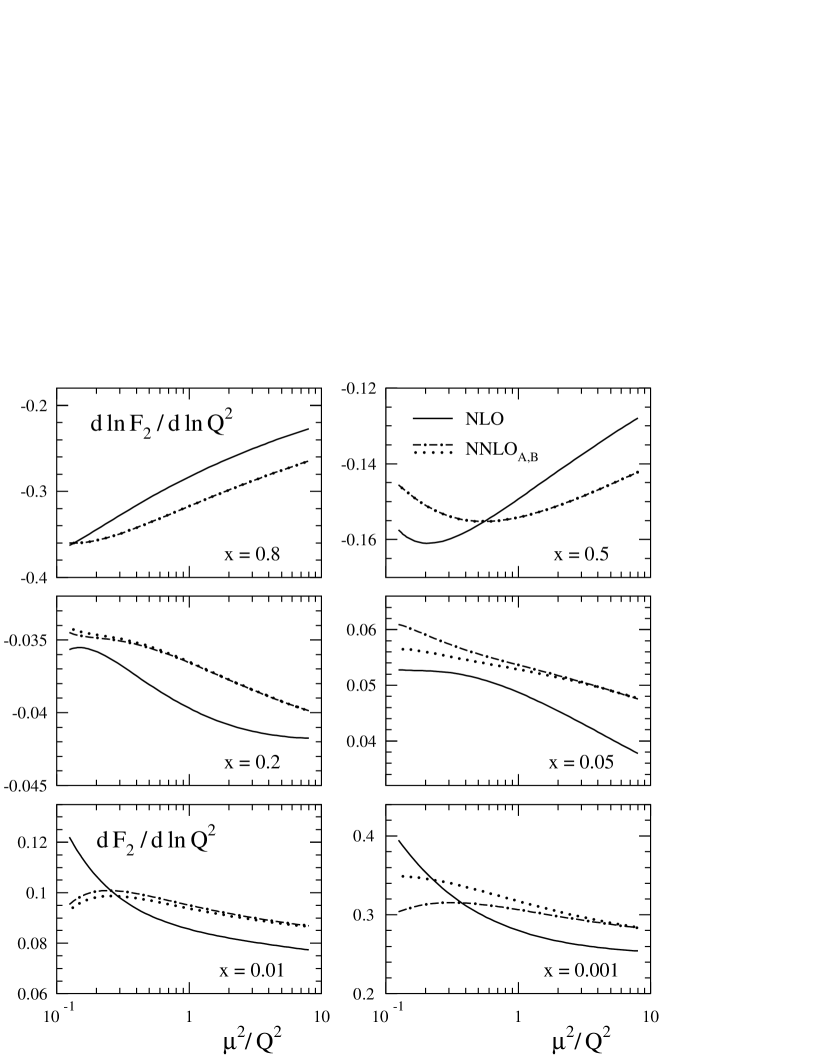
Figure 12: As Fig. 11, but for the logarithmic derivative $\dot{F}_{2}$ (upper four $x$-bins) and the linear derivative $F_{2}^{\,\prime}$ (lower two values of $x$).

Figure 13: The relative scale uncertainties of the NLO and NNLO predictions for $F_{2}(x,Q^{2})$ and its linear (small $x$) and logarithmic (large $x$) $Q^{2}$-derivatives at $Q^{2}\simeq 30\mbox{ GeV}^{2}$, as estimated by the quantities $\Delta F_{2}$, $\Delta F_{2}^{\,\prime}$ and $\Delta\dot{F}_{2}$ defined in Eq. (5.4).

It is also interesting to consider separately the dependence of $F_{2}$ and its derivatives on the renormalization scale $\mu_{r}$ (keeping $\mu_{f}^{2}=Q^{2}=\mu_{f,0}^{2}$) and on the factorization scale $\mu_{f}$ (keeping $\mu_{r}^{2}=Q^{2}=\mu_{f,0}^{2}$). For $F_{2}$ the resulting variations are comparable over the full $x$-range at NNLO. At $x=0.8$, for example, they are both about half as large as the $\mu$-dependence shown in Fig. 11. It is worth noting that the $\mu_{r}$-variation of $F_{2}$ at small-$x$ worsens by the transition from NLO to NNLO, despite the fact that a renormalization scale logarithm enters for the first time only at NNLO, see Eqs. (2.16) and (2.18). This is due to the large contribution of $c_{2,g}^{(2)}$ shown in Fig. 10. When both scales are varied, however, this deterioration is overcompensated by the clear improvement of the $\mu_{f}$-dependence. For the $Q^{2}$-derivatives of Fig. 12 the effect of $\mu_{f}$ is much smaller than that of $\mu_{r}$, except for the NLO case at small $x$ (where the large scale dependence of $\dot{\Sigma}$ of Fig. 9 is relevant). At NNLO the dependence on $\mu_{f}$ is relatively largest at very large $x$, but even at $x=0.8$ it does not exceed a quarter of the $\mu$-variation shown in Fig. 12.

So far the NNLO effects have been discussed for the fixed initial parton densities $\Sigma(x,\mu_{f,0}^{2})$ and $g(x,\mu_{f,0}^{2})$ of Eq. (5.1) and the coupling constant $\alpha_{s}(\mu_{f,0}^{2})=0.2$. We now finally address the impact of the NNLO terms on the determination of these perturbatively incalculable inputs from data on $F_{2}$. For a simple estimate of the resulting difference between the NLO and the NNLO singlet parton densities and their respective theoretical uncertainties, we employ as ‘data’ the values of $F_{2}(x,Q^{2})$ and $F_{2}^{\,\prime}(x,Q^{2})$ for $Q^{2}=\mu_{f,0}^{2}\simeq 30\mbox{ GeV}^{2}$ at the six $x$-values of Figs. 11 and 12, supplemented by $x=10^{-4}$. I.e., the parameters of the input (5.1) (including a $(1+Ax)$ interpolation term for the gluon density, but imposing the momentum sum rule) are fitted at NNLO for $\mu^{2}=Q^{2}$ to the corresponding NLO results. The errors bands due to the scale dependence are then determined by repeating the NLO and NNLO fits to their respective $\mu^{2}\!=\!Q^{2}$ central values of $F_{2}$ and $F_{2}^{\,\prime}$ for $\mu^{2}/Q^{2}=$ 0.25, 0.5, 2 and 4.

A critical point in analyses of $F_{2,S}$ is the correlation between $\alpha_{s}$ and the gluon density, which tends to strongly increase the $\mu$-variation of the fitted values of $\alpha_{s}$. Indeed, under the present conditions this variation is enhanced, in both NLO and NNLO, by about a factor of two with respect to an analogous analysis of the non-singlet structure function $F_{2,\rm NS}$, thus preventing an accurate determination of $\alpha_{s}$ from $F_{2,S}$ alone. In order to keep the scale variation of $\alpha_{s}$ at a level realistic for analyses of data on electromagnetic DIS (where both $F_{2,\rm NS}^{\,p}$ and $F_{2,\rm S}^{\,p}$ have been accurately measured), we therefore take over the values for $\alpha_{s}(\mu_{f,0}^{2})$ from our previous non-singlet analysis [6]: $\alpha_{s}(\mu_{f,0}^{2})$ = 0.188, 0.200 and 0.220, respectively, for $\mu^{2}=0.25\,Q^{2}$, $Q^{2}$ and $4\,Q^{2}$ and NLO. The corresponding NNLO values read 0.190, 0.194 and 0.202. It is clear from our discussion above that these scale uncertainties of $\alpha_{s}$ are almost entirely due to the variation of the renormalization scale.

The resulting NNLO central values and NLO and NNLO scale-uncertainty bands for $\Sigma(x,\mu_{f,0}^{2})$ and $g(x,\mu_{f,0}^{2})$ are presented in Fig. 14. The shift of $\Sigma_{\rm NNLO}$ with respect to $\Sigma_{\rm NLO}$ – an enhancement between 3% and 7% at small $x$, and a sizeable decrease at very large $x$ reaching 13% at $x=0.8$ – rather directly reflects the results for $F_{2}$ shown in Fig. 10. Likewise the reduction of the scale dependence to $\pm 2\%$ or less for $10^{-3}\!<x<0.5$ closely follows the pattern of $\Delta F_{2}$ in Fig. 13. The corresponding results for the gluon density, on the other hand, are considerably affected by the values of $\alpha_{s}$. In fact, the theoretical error band for $g_{\rm NNLO}^{\,}$ does not exceed 2% for $3\!\cdot\!10^{-3}\!<x<0.2$. For $x<10^{-3}$ the present uncertainties of the three-loop splitting functions prevent an improvement on the rather accurate NLO determination of the gluon density.

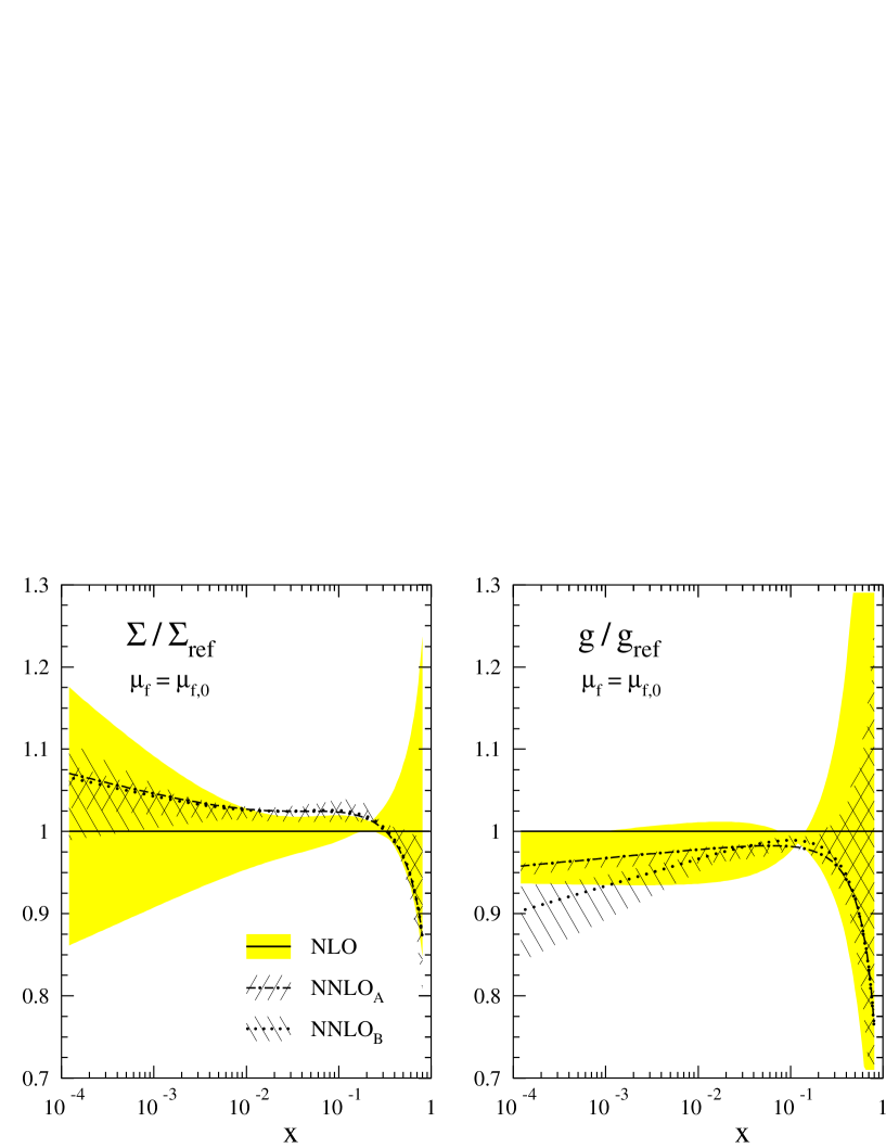
Figure 14: Comparison of the NLO and NNLO singlet quark and gluon densities and their scale-uncertainty bands as obtained by fitting $F_{2}$ and $F_{2}^{\,\prime}$ at $Q^{2}=\mu_{f,0}^{2}\simeq 30\mbox{ GeV}^{2}$ for $10^{-4}\leq x\leq 0.8$. The range of scales used for the error bands is $0.25\,Q^{2}\leq\mu^{2}\leq 4\,Q^{2}$.

6 Summary

We have investigated the effect of the NNLO perturbative QCD corrections on the evolution of the unpolarized flavour-singlet quark and gluon densities, $\Sigma(x,\mu_{f}^{2})$ and $g(x,\mu_{f}^{2})$, and on the most important singlet structure function, $F_{2,S}(x,Q^{2})$. Our main new ingredients are approximate expressions for the $x$-dependence $P_{ij}^{(2)}(x)$ of the singlet three-loop splitting functions, including quantitative estimates of their residual uncertainties. These parametrizations have been derived from the lowest four even-integer moments $P_{ij}^{(2)}(N)$, $N=2$, 4, 6 and 8, calculated in ref. [8], supplemented by the results of refs. [11, 12] for the leading small-$x$ terms $\propto(1/x)\ln x$ of $P_{qq}^{(2)}$, $P_{qg}^{(2)}$ and $P_{gg}^{(2)}$. Consequently the differences between our parametrizations illustrated in Figs. 3 and 4 oscillate at large $x$, as the difference between any two approximations obviously has four vanishing moments. At $x\,\raisebox{-1.9919pt}{$\>\stackrel{{\scriptstyle<}}{{{\scriptstyle\sim}}}\>$}\,10^{-2}$ the differences increase, because the $(1/x)\ln x$ terms unfortunately do not sufficiently dominate over the unknown less singular contributions like $1/x$ in the experimentally accessible region of small $x$, see also refs. [24, 35].

Clearly our parametrizations represent only a temporary ‘solution’ of the problem of the three-loop splitting functions, which will be superseded sooner or later by an exact calculation. However, for two reasons the present approach is, over a wide region of $x$, much more effective than a brief look at Figs. 3 and 4 might suggest. First of all the splitting functions enter physical quantities only via convolutions with nonperturbative initial distributions, which smoothen out the above-mentioned oscillations to a large extent. While this mechanisms leads to especially small uncertainties at $x\,\raisebox{-1.9919pt}{$\>\stackrel{{\scriptstyle>}}{{{\scriptstyle\sim}}}\>$}\,0.1$, the convolutions extend the relevance of the large-$x$ constraints [8] deep into the small-$x$ region as exemplified in the discussion of Fig. 2. The second reason is that the series expansion for the evolution of the parton densities is very well converging — except, possibly, at $x<10^{-3}$. Choosing for definiteness $\alpha_{s}=0.2$ for the strong coupling constant (this corresponds to a scale between about 20 GeV² and 50 GeV², depending on the precise value of $\alpha_{s}(M_{Z}^{2})^{\,}$) the NNLO effect on the evolution of $\Sigma(x,\mu_{f}^{2})$ and $g(x,\mu_{f}^{2})$ amounts to less than 2% and 1%, respectively, at $x\,\raisebox{-1.9919pt}{$\>\stackrel{{\scriptstyle>}}{{{\scriptstyle\sim}}}\>$}\,0.2$. Hence the net uncertainties due to the incomplete information on the $P_{ij}^{(2)}(x)$ are absolutely negligible in this region as shown in Figs. 5 and 6. Of course, these uncertainties rise towards small $x$, but they exceed $\pm 2\%$ only below $x\simeq 10^{-3}$ (or a few times this number, if much lower scales are involved), leaving a comfortably large region of safe applicability of our results to processes at the Tevatron and the LHC.

At $x\,\raisebox{-1.9919pt}{$\>\stackrel{{\scriptstyle>}}{{{\scriptstyle\sim}}}\>$}\,0.2$ the NNLO renormalization-scale variation (for the conventional interval $\frac{1}{4}\,\mu_{f}^{2}\leq\mu_{r}^{2}\leq 4\,\mu_{f}^{2}$) amounts to less than 2% and 1%, respectively, for $d\Sigma/d\ln\mu_{f}^{2}$ and $dg/d\ln\mu_{f}^{2}$ at our reference point $\mu_{f}^{2}\simeq 30$ GeV². The corresponding numbers at $x=10^{-3}$ read 5% and 3%. Except for the gluon evolution at this latter value of $x$, these results represent an improvement on the NLO evolution by a factor of three or more. Taking into account also the rapid convergence at $\mu_{r}=\mu_{f}$ and our corresponding findings for the non-singlet sector in ref. [6], we expect that terms beyond NNLO will affect the parton evolution by less than 1% at large $x$ and less than 2% down to $x\simeq 10^{-3}$ for $\alpha_{s}\simeq 0.2$.

Due to the additional effect of the two-loop coefficient functions [2, 3], the structure function $F_{2,S}$ and its scaling violations receive considerably larger NNLO corrections at $x>10^{-2}$. In fact, keeping only the coefficient functions (and omitting the three-loop splitting functions $P_{ij}^{(2)}(x)$ altogether) forms quite a good approximation in this $x$-range. As shown in Fig. 10, the NNLO corrections for both $F_{2}$ and its $Q^{2}$-derivative are particularly large at very large $x$, e.g., 15% for $F_{2,S}$ and 11% for $d\ln F_{2,S}/d\ln Q^{2}$ at $x=0.8$ for our reference scale $Q^{2}\simeq 30\mbox{ GeV}^{2}$. This is an effect of the large soft-gluon terms in the quark coefficient functions which are not special to the singlet case considered here. While the gluon contributions dominates the sizeable (up to about 7%) NNLO corrections at small $x$, their effect is suppressed at large $x$, especially for the absolute size of $F_{2,S}$. It is worth noting, however, that that the gluon contribution to $dF_{2,S}/d\ln Q^{2}$ at $x=0.5$ still amounts to 5% at NNLO (40% more than at NLO), an effect large enough to jeopardize analyses which apply a purely non-singlet formalism to the data on the proton structure function $F_{2}^{\,p}(x,Q^{2})$ in the region $x>0.3$. The accuracies of both $F_{2}$ and its scaling violations, as estimated by the scale dependence, are considerably improved (by more than a factor of two over a wide region) by the inclusion of the NNLO terms. Consequently the same applies to the theoretical accuracy of determinations of the singlet quark and gluon densities from data on $F_{2,S}$ and $dF_{2,S}/d\ln Q^{2}$ at $Q^{2}\simeq 30\mbox{ GeV}^{2}$ illustrated in Fig. 14: uncertainties of less than 2% from the truncation of the perturbation series are obtained for the quark density at $10^{-3}\!<\!x\!<\!0.5$ and for for the gluon density at $3\cdot 10^{-3}\!<\!x\!<\!0.2$.

Our results of ref. [6] and the present paper complete, if only approximately at $x\!>\!10^{-3}$, the theoretical prerequisites for NNLO analyses of structure functions in DIS and total cross sections of Drell-Yan processes. Further progress at large $x$ — especially a further improvement on the theoretical accuracy of NNLO $\alpha_{s}$-determinations from structure functions [36, 37, 6] — can be obtained by including the $O(\alpha_{s}^{3})$ coefficient functions, particularly in the non-singlet sector dominating the extraction of $\alpha_{s}$. In fact, results on these functions are available from the fixed-moment calculations of refs. [7, 8] and from soft-gluon resummation [38, 39]. We will address this issue in a forthcoming publication. Progress towards the important HERA small-$x$ region of $x\raisebox{-1.9919pt}{$\>\stackrel{{\scriptstyle<}}{{{\scriptstyle\sim}}}\>$}10^{-3}$ at moderate to low $Q^{2}$, however, definitely requires the full calculation of the three-loop splitting functions.

Fortran subroutines of our parametrizations of $c_{a,i}^{(2)}(x)$ ($a=2,L$; $i=q,g$) and $P_{ij}^{(2)}(x)$ can be obtained via email to neerven@lorentz.leidenuniv.nl or avogt@lorentz.leidenuniv.nl.

Appendix: The singlet coefficient functions in $N$-space

The Mellin transforms (2.12) of the parametrizations (3.3)–(3.6) of the two-loop singlet coefficient functions for $F_{L}$ and $F_{2}$ are given in terms of the integer-$N$ sums $S_{l}(N)$ and their complex-$N$ analytic continuations

$$S_{l}\equiv S_{l}(N)=\sum_{k=1}^{N}\frac{1}{k^{l}}=\zeta(l)-\frac{(-1)^{l}}{(l-1)!}\,\psi^{(l-1)}(N\!+\!1)\>\>.$$ (A.1)

Here $\zeta(1)$ represents the Euler–Mascheroni constant, and $\zeta(l\!>\!1)$ Riemann’s $\zeta$-function. The $l\,$th logarithmic derivative $\psi^{(l-1)}$ of the $\Gamma$-function can be readily evaluated using the asymptotic expansion for ${\rm Re}\,N>10$ together with the functional equation.

The moments (2.12) of the pure singlet coefficient functions (3.3) and (3.4) are given by

$$c_{L,{\rm PS}}^{(2)}(N)\! = N_{f}\,\Bigg{\{}\bigg{(}-\frac{15.94}{N}+\frac{37.092}{N+1}-\frac{26.364}{N+2}+\frac{5.212}{N+3}\bigg{)}S_{1}$$ (A.2)

$$\mbox{}-\frac{2.370}{N-1}+\frac{0.842}{N^{3}}-\frac{28.09}{N^{2}}+\frac{26.38}{N}+\frac{3.040}{(N+1)^{3}}+\frac{65.182}{(N+1)^{2}}$$

$$\mbox{}-\frac{88.678}{N+1}-\frac{26.364}{(N+2)^{2}}+\frac{91.756}{N+2}+\frac{5.212}{(N+3)^{2}}-\frac{27.088}{N+3}\Bigg{\}}$$

and

$$c_{2,{\rm PS}}^{(2)}(N)\! = N_{f}\,\Bigg{\{}\bigg{(}\frac{49.702}{N}-\frac{27.802}{N+1}\bigg{)}S_{3}+\bigg{(}\frac{49.5}{N^{2}}+\frac{30.23}{N}-\frac{27.903}{(N+1)^{2}}\bigg{)}S_{2}$$ (A.3)

$$\mbox{}+0.101\bigg{(}\frac{1}{N}-\frac{1}{N+1}\bigg{)}\Big{(}3\,S_{2}S_{1}+S_{1}^{3}\Big{)}+\bigg{(}\frac{49.5}{N^{3}}+\frac{30.23}{N^{2}}-\frac{28.206}{(N+1)^{3}}\bigg{)}S_{1}$$

$$\mbox{}+\frac{5.290}{N-1}-\frac{25.86}{N^{4}}-\frac{4.172}{N^{3}}-\frac{121.205}{N^{2}}-\frac{114.519}{N}-\frac{83.406}{(N+1)^{4}}$$

$$\mbox{}+\frac{45.4003}{(N+1)^{2}}+\frac{33.1769}{N+1}\Bigg{\}}\>\>.$$

The corresponding expressions for the gluon coefficient functions (3.5) and (3.6) read

$$c_{L,g}^{(2)}(N)\! = N_{f}\,\Bigg{\{}\bigg{(}\frac{94.74}{N}+\frac{1017.06}{N+1}+\frac{49.20}{N+2}\bigg{)}S_{2}+\bigg{(}\frac{94.74}{N}-\frac{143.94}{N+1}+\frac{49.20}{N+2}\bigg{)}S_{1}^{2}$$ (A.4)

$$\mbox{}+\bigg{(}-\frac{864.8}{N}+\frac{873.12}{(N+1)^{2}}+\frac{963.2}{N+1}+\frac{98.40}{(N+2)^{2}}-\frac{98.40}{N+2}\bigg{)}S_{1}$$

$$\mbox{}-\frac{5.333}{N-1}-\frac{39.66}{N^{2}}+\frac{5.333}{N}+\frac{2154.24}{(N+1)^{3}}+\frac{1002.86}{(N+1)^{2}}-\frac{1909.768}{N+1}$$

$$\mbox{}-\frac{98.40}{(N+2)^{3}}+\frac{98.40}{(N+2)^{2}}\Bigg{\}}$$

and

$$c_{2,g}^{(2)}(N)\! = N_{f}\,\Bigg{\{}\bigg{(}\frac{2760.11}{N}+\frac{418.8}{N+1}\bigg{)}S_{3}+\bigg{(}\frac{2320}{N^{2}}-\frac{24}{N}+\frac{628.2}{(N+1)^{2}}\bigg{)}S_{2}$$

$$\mbox{}+\bigg{(}\frac{1096.07}{N}+\frac{628.2}{N+1}\bigg{)}S_{2}S_{1}+\bigg{(}\frac{871.8}{N^{2}}-\frac{24}{N}+\frac{628.2}{(N+1)^{2}}\bigg{)}S_{1}^{2}$$

$$\mbox{}-\bigg{(}\frac{1494}{N\!-\!1}-\frac{1448.20}{N^{3}}+\frac{1385.12}{N}-\frac{1256.4}{(N\!+\!1)^{3}}\bigg{)}S_{1}-\bigg{(}\frac{215.845}{N}-\frac{209.4}{N\!+\!1}\bigg{)}S_{1}^{3}$$

$$\mbox{}+\frac{1505.9}{N-1}-\frac{31.914}{N^{4}}-\frac{118.96}{N^{3}}-\frac{2097.4}{N^{2}}-\frac{4938.34}{N}+\frac{1256.4}{(N+1)^{4}}-0.271\Bigg{\}}\>\>.$$

Let us finally briefly elaborate on the derivation of Eq. (4.7) from Eq. (4.5). The exact expression [2, 3] for the residue of the $N=1$ pole of $c_{2,g}^{(2)}(N)$ reads $N_{f}\,[344/9-16\,\zeta(2)]$. Recalling that the Mellin transform of $(1/x)\ln x$ is given by $-1/(N\!-\!1)^{2}$, this information combined with the corresponding term $16/[3(N\!-\!1)]$ of the LO splitting function $P_{gq}^{(0)}$ is sufficient to obtain Eq. (4.7) from Eqs. (4.5) and (4.6). The latter relation simply arises since the other contributions to the scheme transformation (2.24) do not lead to any $1/(N\!-\!1)^{2}$ terms.

References

• [1] W. Furmanski and R. Petronzio, Z. Phys. C11 (1982) 293; and references therein
• [2] E.B. Zijlstra and W.L. van Neerven, Phys. Lett. B272 (1991) 127; ibid. B273 (1991) 476; ibid. B297 (1992) 377
• [3] E.B. Zijlstra and W.L. van Neerven, Nucl. Phys. B383 (1992) 525;
E.B. Zijlstra, thesis, Leiden University 1993
• [4] R. Hamberg, W.L. van Neerven and T. Matsuura, Nucl. Phys. B359 (1991) 343;
R. Hamberg, thesis, Leiden University 1991;
W.L. van Neerven and E.B. Zijlstra, Nucl. Phys. B382 (1992) 11
• [5] J.A.M. Vermaseren and S. Moch, preprint NIKHEF-00-008 (hep-ph/0004235)
• [6] W.L. van Neerven and A. Vogt, Nucl. Phys. B568 (2000) 263
• [7] S.A. Larin, T. van Ritbergen, and J.A.M. Vermaseren, Nucl. Phys. B427 (1994) 41
• [8] S.A. Larin, P. Nogueira, T. van Ritbergen, and J.A.M. Vermaseren, Nucl. Phys. B492 (1997) 338;
T. van Ritbergen, thesis, Amsterdam University 1996
• [9] J. A. Gracey, Phys. Lett. B322 (1994) 141
• [10] J. Blümlein and A. Vogt, Phys. Lett. B370 (1996) 149
• [11] S. Catani and F. Hautmann, Nucl. Phys. B427 (1994) 475
• [12] V.S. Fadin and L.N. Lipatov, Phys. Lett. B429 (1998) 127; and references therein
• [13] J.F. Bennett and J.A. Gracey, Nucl. Phys. B517 (1998) 241
• [14] A.D. Martin, R.G. Roberts and W.J. Stirling, Phys. Lett. B387 (1996) 419;
A.D. Martin, R.G. Roberts, W.J. Stirling and R.S. Thorne, Eur. Phys. J. C4 (1998) 463
• [15] H.L. Lai et al., CTEQ Collab., Phys. Rev. D55 (1997) 1280; Eur. Phys. J. C12 (2000) 375
• [16] M. Glück, E. Reya and A. Vogt, Z. Phys. C67 (1995) 433; Eur. Phys. J. C5 (1998) 461
• [17] J. Sanchez Guillen et al., Nucl. Phys. B353 (1991) 337
• [18] R. Hamberg and W.L. van Neerven, Nucl. Phys. B379 (1992) 143
• [19] O.V. Tarasov, A.A. Vladimirov, and A.Yu. Zharkov, Phys. Lett. B93 (1980) 429;
S.A. Larin and J.A.M. Vermaseren, Phys. Lett. B303 (1993) 334
• [20] M. Diemoz, F. Ferroni, E. Longo and G. Martinelli, Z. Phys. C39 (1988)
• [21] S. Moch and J.A.M. Vermaseren, Nucl. Phys. B573 (2000) 853
• [22] M. Glück, E. Reya and A. Vogt, Z. Phys. C48 (1990) 471;
Ch. Berger, D. Graudenz, M. Hampel and A. Vogt, Z. Phys. C70 (1996) 77;
D. A. Kosower, Nucl. Phys. B506 (1997) 439; ibid. B520 (1998) 263
• [23] J. Blümlein and S. Kurth, preprint DESY 97-160 (hep-ph/9708388); Phys. Rev. D60 (1999) 014018;
J. Blümlein, preprint DESY 98-149 (hep-ph/0003100)
• [24] J. Blümlein and A. Vogt, Phys. Rev. D57 (1998) 1; ibid. D58 (1998) 014020;
J. Blümlein, V. Ravindran, W.L. van Neerven and A. Vogt, Proceedings of DIS 98, Brussels, April 1998, eds. Gh. Coremans and R. Roosen (World Scientific 1998), p. 211 (hep-ph/9806368)
• [25] R. Mertig and W.L. van Neerven, Z. Phys. C70 (1996) 637
• [26] W. Vogelsang, Phys. Rev. D54 (1996) 2023; Nucl. Phys. B475 (1996) 47
• [27] W. Furmanski and R. Petronzio, Phys. Lett. B97 (1980) 437
• [28] G. Curci, W. Furmanski and R. Petronzio, Nucl. Phys. B175 (1980) 27
• [29] R.K. Ellis and W. Vogelsang, preprint CERN-TH-96-50 (hep-ph/9602356)
• [30] L.V. Avdeev and A.A. Vladimirov, Nucl. Phys. B219 (1983) 262
• [31] Y. Matiounine, J. Smith and W.L. van Neerven, Phys. Rev. D57 (1998) 6701
• [32] J. Blümlein, S. Riemersma and A. Vogt, Nucl. Phys. (Proc. Suppl.) 51C (1996) 30 (hep-ph/9608470)
• [33] A. Chuvakin, J. Smith and W.L. van Neerven, Phys. Rev. D61 (2000) 096004; and references therein
• [34] W.L. van Neerven, talk at the 1993 DESY Workshop on QCD.
• [35] J. Blümlein and W.L. van Neerven, Phys. Lett. B450 (1999) 412
• [36] A.L. Kataev, A.V. Kotikov, G. Parente and A.V. Sidorov, Phys. Lett. B388 (1996) 179; ibid. B417 (1998) 374;
A.L. Kataev, G. Parente, A.V. Sidorov, Nucl. Phys. B573 (2000) 405
• [37] J. Santiago and F.J. Yndurain, Nucl. Phys. B563 (1999) 45; Madrid University preprint FTUAM-99-17 (hep-ph/9907387)
• [38] G. Sterman, Nucl. Phys. B281 (1987) 310;
S. Catani and L. Trentadue, Nucl. Phys. B327 (1989) 323; ibid. B353 (1991) 183
• [39] A. Vogt, Phys. Lett. B471 (1999) 97