McGill 00-15

NORDITA 2000/38 HE

LPT-ORSAY 00-46

hep-ph/0006119

Supersymmetric Electroweak Baryogenesis

James M. Cline

McGill University, Montréal, Québec H3A 2T8, Canada
Michael Joyce

LPT, Université Paris-XI, Bâtiment 211, F-91405 Orsay Cedex, France
Kimmo Kainulainen

NORDITA, Blegdamsvej 17, DK-2100, Copenhagen Ø, Denmark

We re-examine the generation of the baryon asymmetry in the minimal supersymmetric standard model (MSSM) during the electroweak phase transition. We find that the dominant source for baryogenesis arises from the chargino sector. The CP-violation comes from the complex phase in the $\mu$ parameter, which provides CP-odd contributions to the particle dispersion relations. This leads to different accelerations for particles and antiparticles in the wall region which, combined with diffusion, leads to the separation of Higgsinos and their antiparticles in the front of the wall. These asymmetries get transported to produce perturbations in the left-handed chiral quarks, which then drive sphaleron interactions to create the baryon asymmetry. We present a complete derivation of the semiclassical WKB formalism, including the chargino dispersion relations and a self-consistent derivation of the diffusion equations starting from semiclassical Boltzmann equations for WKB-excitations. We stress the advantages of treating the transport equations in terms of the manifestly gauge invariant physical energy and kinetic momentum, rather than in the gauge variant canonical variables used in previous treatments. We show that a large enough baryon asymmetry can be created for the phase of the complex $\mu$-parameter as small as $\sim 10^{-3}$, which is consistent with bounds from the neutron electric dipole moment.

1 Introduction

It is a fascinating possibility that the baryon asymmetry of the universe (BAU) may have been generated at the electroweak epoch (for reviews, see [2]). The great attraction of this idea is that, in contrast to other mechanisms operating at higher energy scales, it involves physics which is being searched for at accelerators now. An a priori calculation of the baryon asymmetry, as accurate as that of the abundance of the light elements in nucleosynthesis, may still be unattainable at present, but we should nevertheless strive to compute it as carefully as possible. One hopes thereby to reach a definitive conclusion as to the feasibility, at least, of generating the BAU at the electroweak scale.

While there are many theoretical motivations for considering extensions of the standard model (SM), in the present context we are also prompted to do so for the simple reason that the SM by itself appears unable to produce the observed BAU. The smallness of the CP violation in the KM matrix appears to be in itself an insurmountable obstacle to baryogenesis in the SM (although there has been considerable debate on this subject [3]), and has motivated many studies of baryogenesis in extended models with additional CP violation leading to more efficient baryon production. In addition to this problem, moreover, the SM fails badly with respect to the sphaleron wash-out bound. Lattice studies have shown that for any value of the higgs mass, even well below the present experimental lower limit, the phase transition would be so weak that sphaleron interactions remain in equilibrium in the broken phase of the electroweak sector, causing the baryon asymmetry to relax back to essentially zero immediately after its generation [5].

Several extensions of the SM have been considered to overcome the sphaleron wash-out bound by strengthening the phase transition [6, 7, 8, 9]. Best motivated from the particle physics point of view is the minimal supersymmetric standard model (MSSM). Several recent perturbative and nonperturbative studies of the properties of the phase transition in this model [10, 11, 12, 13] have shown that in a restricted part of the parameter space, the sphaleron bound can be satisfied. An important question is therefore whether for these same parameter values the generation of the observed BAU is possible.

Baryogenesis in the MSSM has already been studied in several papers [14, 15, 16, 17, 18, 19, 20, 21, 22, 23]. The overall framework of the baryogenesis mechanism is essentially agreed upon: bubbles nucleate at a first order phase transition and the expanding bubble walls propagate through the hot plasma, perturbing the quasiparticle distributions from equilibrium in a CP-violating manner. Incorporating the effects of transport leads to a local excess or deficit of left-handed fermions over their antiparticles on and around the propagating bubble walls. This drives the anomalous baryon number violating processes to produce a net baryon asymmetry, which is swept behind the bubble wall where it is frozen in (assuming that the sphaleron bound is satisfied). Moveover, common to all methods is reducing the problem to a set of diffusion equations coupling the sourced species to the species that bias the sphalerons. These are coupled equations which have the general form

$$D_{i}\xi_{i}^{\prime\prime}+v_{w}\xi^{\prime}+\Gamma_{i}(\xi_{i}+\xi_{j}+\cdots)=S_{i}\;,$$ (1)

where $i$ labels the particle species and $\xi=\mu_{i}/T$ is its chemical potential divided by temperature. Primes denote spatial derivatives in the direction ($z$) perpendicular to the wall, $v_{w}$ is the wall velocity, $\Gamma_{i}$ is the rate of an interaction that converts species $i$ into other kinds of particles, and $S_{i}$ is the source term associated with the current generated at the bubble wall. There is little controversy about the form of these equations, but little agreement exists as to how to properly derive the source terms $S_{i}$. There are many different formalisms for obtaining the sources [25, 7, 26], but so far little effort has been made to see how far they agree or disagree with each other. We shall comment on this issue briefly in our conclusions.

Here we shall use the ‘classical force’ mechanism (CFM) for baryogenesis [7], [19, 21, 22]. The CFM makes use of the intuitively simple picture of particles being transported in the plasma under the influence of the classical force exerted on them by the spatially varying Higgs field condensate. We assume that the plasma in this bubble wall region can be described by a collection of semiclassical quasiparticle states which we shall refer to as WKB states, because their equation of motion is derived using the WKB approximation expanding in derivatives of the background field. The force acting on the particles can be deduced from the WKB dispersion relations and their corresponding canonical equations of motion. This is a reasonable assumption when the de Broglie wavelength of the states is much shorter than the scale of variation of the bubble wall, i.e. $\lambda\ll\ell_{w}$, which is satisfied in electroweak baryogenesis; in the MSSM, the wall widths are typically $\ell_{w}\sim 6-14/T$ [13, 27], whereas for a typical excitation $\lambda\sim 1/T$. Given these conditions one can write a semiclassical Boltzmann equation for the distribution functions of the local WKB-states

$$(\partial_{t}+{\bf v}_{g}\cdot\partial_{\bf x}+{\bf F}\cdot\partial_{\bf p})f_{i}=C[f_{i},f_{j},...].$$ (2)

where the group velocity and classical force are given respectively by

$${\bf v}_{g}\equiv\partial_{{\bf p}_{c}}\omega;\qquad{\bf F}=\dot{\bf p}=\omega\dot{\bf v}_{g}.$$ (3)

Here ${\bf p}_{c}$ is the canonical, and ${\bf p}\equiv\omega{\bf v}_{g}$ the physical, kinetic momentum along the WKB worldline. Note that we treat the transport problem here in the kinetic variables - in which the Boltzmann equation has the non-canonical form of (2) - rather than in the canonical variables used in previous treatments. As will be discussed in more detail below, this choice has the simple advantage of circumventing all the difficulties associated with the variance of the canonical variables under local phase (‘gauge’) transformations of the fields in the Lagrangian. In these kinetic variables it is also more manifestly (and gauge independently) clear how, because of CP-violating effects, particles and antipartices experience different forces in the wall region, which leads to the separation of chiral currents. The explicit form of ${\bf v}_{g}$ and ${\bf F}$ in a given model can be found from the WKB dispersion relations, as we will illustrate in sections 2 and 3. The Boltzmann equation (2) can then be converted to diffusion equations in a standard way by doing a truncated moment expansion [19] (see section 4).

The largest contribution to baryogenesis in the MSSM comes from the chargino and neutralino sectors. For the charginos, the CP violating effects are due to the complex parameters $m_{2}$ and $\mu$ in the mass term

$$\bar{\psi}_{R}M\psi_{L}=(\overline{\widetilde{w}^{{}^{+}}},\ \overline{\widetilde{h}^{{}^{+}}}_{1})_{R}\left(\begin{array}[]{cc}m_{2}&gH_{2}\\ gH_{1}&\mu\end{array}\right)\left(\begin{array}[]{c}\widetilde{w}^{{}^{+}}\\ \widetilde{h}^{{}^{+}}_{2}\end{array}\right)_{\!\!L}.$$ (4)

The complex phases, combined with the mixing due to the Higgs fields, which vary inside the bubble wall, give rise to spatially varying effective phases for the mass eigenstates, which induce CP-violating currents for these excitations. To get analytic results, one can try to compute the current to leading order in an expansion in derivatives of the Higgs fields. This is the procedure followed in all methods designed to work on the thick wall limit [25, 7, 26, 19]. This approximation cannot be used in the quantum reflection case [8, 17, 9, 20], which can be relevant in the limit of very thin bubble walls.

We comment here on an apparent discrepancy in the literature concerning the derivative expansion of the chargino source. References [15] and [18] obtained a source for the $H_{1}-H_{2}$ combination of Higgs currents of the form

$$S_{H_{1}-H_{2}}\sim{\rm Im}(m_{2}\,\mu)\,(H_{1}H_{2}^{\prime}-H_{2}H_{1}^{\prime}),$$ (5)

whereas ref. [19] found the other orthogonal linear combination, $H_{1}H_{2}^{\prime}+H_{2}H_{1}^{\prime}$. We previously believed that the disagreement was because of fundamental differences between our CFM formalism and those of refs. [15, 25, 18, 26]. However we recently understood [21, 22] that the difference was partially due to the fact that we were in fact computing the source for $H_{1}+H_{2}$, for which the result is

$$S_{H_{1}+H_{2}}\sim{\rm Im}(m_{2}\,\mu)\,(H_{1}H_{2}^{\prime}+H_{2}H_{1}^{\prime}),$$ (6)

Therefore the disagreement about the sign was spurious: it can be shown that all three methods actually agree with eq. (6); it simply was not computed by the other references [15, 18, 26, 20].

The reason that the combination $H_{1}+H_{2}$ was not considered by other authors is that it tends to be suppressed by Yukawa and helicity-flipping interactions from the $\mu$ term in the chargino mass matrix. Let us define chemical potentials for $H_{1}$, $H_{2}$, left-handed third generation quarks $q_{3}$ and right-handed top quarks $t$, which we will assume are equal to the chemical potentials for the corresponding supersymmetric partners, as a consequence of supergauge interactions mediated by gauginos. If all the interactions arising from the Lagrangian

$$V = \mu\tilde{h}_{1}\tilde{h}_{2}+yh_{2}\bar{u}_{R}q_{L}+y\bar{u}_{R}\tilde{h}_{2L}\tilde{q}_{L}+y\tilde{u}^{*}_{R}\tilde{h}_{2L}q_{L}$$ (7)

$$- y\mu h_{1}\tilde{q}^{*}_{L}\tilde{u}_{R}+yA_{t}\tilde{q}_{L}h_{2}\tilde{u}^{*}_{R}+\hbox{h.c.},$$

were considered to be in thermal equilibrium, they would give rise to the constraints $\mu_{H_{1}}-\mu_{Q_{3}}+\mu_{T}=0$, $\mu_{H_{2}}+\mu_{Q_{3}}-\mu_{T}=0$ and $\mu_{H_{1}}+\mu_{H_{2}}=0$. If these conditions hold, the effect of the source $S_{H_{1}+H_{2}}$ is clearly damped to zero. However, the rates of the processes coming from (7) are finite, and by studying the diffusion equations one can show that there are corrections of order $(D_{h}\Gamma)^{-1/2}\sim 1$, where we used $D_{h}\simeq 20/T$ and the Yukawa rate $\Gamma\simeq 0.02T$ (see eq. (169) and the discussion following).

Even in formalisms where the source $S_{H_{1}-H_{2}}$ is nonvanishing [18, 26, 20], one should then not neglect the source $S_{H_{1}+H_{2}}$ without first checking whether the other source, $S_{H_{1}-H_{2}}$ really gives a larger effect. In fact $S_{H_{1}-H_{2}}$ does suffer from a severe suppression: quantitative studies of the electroweak bubbles in the MSSM show that the ratio $H_{2}/H_{1}$ remains nearly constant inside the bubble walls [27, 13]; in Monte Carlo searches of the MSSM parameter space, the deviation from constancy is typically at the level of one part in $10^{3}$, and never more than $0.02$. Therefore the source $S_{H_{1}-H_{2}}$ is suppressed from the outset by a factor of $10^{2}-10^{3}$ relative to $S_{H_{1}+H_{2}}$, which is much worse than the Yukawa equilibrium suppression estimated above.

In the CFM the situation concerning the source $S_{H_{1}-H_{2}}$ is even worse: we will show that there will be no source arising from classical force, when computed correctly. To see this is actually quite subtle, and relates to the question of the gauge invariance we have referred to. If the problem is considered solely in terms of the canonical variables, there appears to be a non-trivial source of the form (5). That this term is unphysical however, is indicated by the fact that it can be transformed away by a field redefinition of the form

$$\widetilde{h}^{{}^{+}}_{iL}\to e^{i\alpha_{i}}\widetilde{h}^{{}^{+}}_{iL},$$ (8)

where $\alpha_{i}\sim\int{\rm Im}(m_{2}\mu)(H_{1}^{\prime}H_{2}-H_{2}^{\prime}H_{1})dz$. Below we will see that no such field redefinition has any effect on the physical momenta or currents, and hence should not give rise to a physical force (see also [22]). In our treatment in terms of the gauge invariant kinetic variables this result is evident. In particular then the new source for baryogenesis in the CFM picture found in [23] is absent in our treatment.

Our main result is that baryogenesis remains viable for a large part of the MSSM parameter space, possibly with the explicit CP-violating phase as small as ${\rm arg}(m_{2}\mu)\sim 10^{-3}$. The efficiency depends on the assumed squark spectrum, and the strongest baryoproduction corresponds to the light right-handed stop scenario, which is also independently favored by the sphaleron wash-out constraint [11, 12]. The resulting asymmetry has a complicated dependence on the wall velocity and for some parameters it peaks around the value of $v_{w}\simeq 0.01$ which has been indicated by recent studies of $v_{w}$ [28, 29].

The rest of the paper is structured as follows. In section 2 we consider the simple case of a Dirac fermion with a complex spatially varying mass. We determine the dispersion relation for the two helicities to leading order in Higgs field derivatives, and find from it the group velocity and the physical force acting on a fermion. We also compute and interpret the currents in the absence of collisions and show explicitly how the gauge invariant force can be identified from canonical equations of motion. In section 3 we employ the formalism in the case of the MSSM, in particular, computing the dispersion relations, group velocities and force terms for the charginos. (Squarks and neutralinos are also discussed here.) In section 4 we derive the diffusion equations, complete with the CP-odd source terms from the Boltzmann equations, using a truncated expansion in moments of the distribution functions. In section 5, these general results are applied to find and solve the appropriate set of diffusion equations which determine the chiral quark asymmetry in the MSSM. The rate of baryon production due to the excess of left-handed quarks is also computed in section 5, and our numerical results are given in section 6. In section 7 we present our conclusions, and a discussion of how the present results differ from previously published ones.

2 Introductory example: Fermion with complex mass

To understand some of the subtleties which arise when solving the equations of motion in the WKB approximation, let us first consider the example of a single Dirac fermion with a spatially varying, complex mass,

$$(i\gamma^{\mu}\partial_{\mu}-mP_{R}-m^{*}P_{L})\psi=0;\qquad m=|m(z)|e^{i\theta(z)},$$ (9)

where $P_{R,L}=\frac{1}{2}(1\pm\gamma_{5})$ are the chiral projection operators. We wish to solve eq. (9) approximately in an expansion in gradients of $|m|$ and $\theta$. To simplify the solution we boost to the frame in which the momentum parallel to the wall is zero ($p_{x}=p_{y}=0$) and consider first positive energy eigenstates, $\psi\sim e^{-i\omega t}$. Then, because spin is a good quantum number, we can write the spin eigenstate as a direct product of chirality and spin states

$$\Psi_{s}\equiv e^{-i\omega t}\left(\begin{array}[]{cc}L_{s}\\ R_{s}\end{array}\right)\otimes\chi_{s};\qquad\sigma_{3}\chi_{s}\equiv s\,\chi_{s},$$ (10)

where $R_{s}$ and $L_{s}$ are the relative amplitudes for right and left chirality, respectively (and we are using the chiral representation of the Dirac matrices). Spin $s$ is related to helicity $\lambda$ by $s\equiv\lambda\,{\rm sign}(p_{z})$. Inserting (10) into the Dirac equation (9) then reduces to two coupled complex equations for complex parameters $L_{s}$ and $R_{s}$:

$$(\omega-is\partial_{z})L_{s} = mR_{s}$$ (11)

$$(\omega+is\partial_{z})R_{s} = m^{*}L_{s}.$$ (12)

We can now use eq. (11) to eliminate $R_{s}$ from (12), which then becomes a single second order complex differential equation for $L_{s}$:

$$\left((\omega+is\partial_{z})\frac{1}{m}(\omega-is\partial_{z})-m^{*}\right)L_{s}=0.$$ (13)

To facilitate the gradient expansion, we write the following WKB ansatz for $L_{s}$:

$$L_{s}\equiv we^{i\int^{z}p_{c}(z^{\prime})dz^{\prime}}.$$ (14)

We have suppressed the spin index $s$ in $w$ and $p_{c}$ for simplicity. Inserting (14) into eq. (13) we find the following two coupled equations (real and imaginary parts of (13)):

$$\omega^{2}-|m|^{2}-p_{c}^{2}+(s\omega+p_{c})\theta^{\prime}-\frac{|m|^{\prime}}{|m|}\frac{w^{\prime}}{w}+\frac{w^{\prime\prime}}{w} = 0$$ (15)

$$2p_{c}w^{\prime}+p_{c}^{\prime}w-\frac{|m|^{\prime}}{|m|}(s\omega+p_{c})w-\theta^{\prime}w^{\prime} = 0$$ (16)

While complicated in appearance, eqs. (15-16) are easily solved iteratively. For example, to the lowest order one sets all derivative terms to zero, whereby the first equation immediately gives the usual dispersion relation $\omega^{2}=p_{c}^{2}+|m|^{2}$. It is also easy to extend the dispersion relation to first order in derivatives, because the contributions proportional to $w^{\prime}$ decouple from eq. (15) at this order:

$$p_{c}=p_{0}+s_{\scriptscriptstyle CP}\frac{s\omega+p_{0}}{2p_{0}}\theta^{\prime}+\alpha^{\prime},$$ (17)

where $p_{0}={\rm sign}(p)\sqrt{\omega^{2}-|m|^{2}}$. In(17) we have shown the generalization to antiparticles by including the sign $s_{\scriptscriptstyle CP}$, which is $+1$ for the particle and $-1$ for the antiparticle. This follows from the fact that the Dirac equation for antiparticles is obtained from (9) by the substitution $m\rightarrow-m^{*}$, which changes $\theta$ to $-\theta$. The arbitrary function $\alpha^{\prime}(z)$ reflects the ambiguity in the definition of momentum $p_{c}$ in (14), because of the freedom to perform vector-like phase redefinitions of the field, $\psi\rightarrow e^{i\alpha(z)}\psi$, which cause $p_{c}\rightarrow p_{c}+\alpha^{\prime}$. This ‘gauge’ dependence reflects the fact that $p_{c}$ is not the physical momentum of the WKB-state, a quantity which we will explicitly identify and show to be gauge independent below. In the preceeding, we considered the left-handed spinor $L_{s}$. The same procedure applied to $R_{s}$ gives

$$p_{c}=p_{0}+s_{\scriptscriptstyle CP}\frac{s\omega-p_{0}}{2p_{0}}\theta^{\prime}+\alpha^{\prime},$$ (18)

because of the sign difference between eqs. (11) and (12). The factors $(s\omega+p_{c})$ are likewise replaced by $s\omega-p_{c}$ in (15) and (16). In the following we will show that this difference actually does not have any physical effect: the group velocity and force acting on the particle is the same whether one uses (17) or (18). For simplicity we continue to refer to the relations for $L_{s}$ unless the contrary is explicitly stated.

2.1 Canonical equations of motion

As anticipated above $p_{c}$ can be identified as the canonical momentum for the motion of the WKB wave-packets. To see this more clearly, let us first invert (17) to obtain an expression for the invariant energy

$$\omega=\sqrt{(p_{c}-\alpha_{\scriptscriptstyle CP})^{2}+|m|^{2}}-s_{\scriptscriptstyle CP}\frac{s\theta^{\prime}}{2},$$ (19)

where $\alpha_{\scriptscriptstyle CP}\equiv\alpha^{\prime}+s_{\scriptscriptstyle CP}\theta^{\prime}/2$ in the left- and $\alpha_{\scriptscriptstyle CP}\equiv\alpha^{\prime}-s_{\scriptscriptstyle CP}\theta^{\prime}/2$ right chiral sector. (This difference in $\alpha_{\scriptscriptstyle CP}$ has no consequence what follows, which is why we have suppressed the indices referring to chirality). Identifying the velocity of the WKB particle with the group velocity of the wave-packet (corresponding to the stationary phase condition of the WKB-wave) it can be computed as

$$v_{g}=(\partial_{p_{c}}\omega)_{x} = \frac{p_{c}-\alpha_{\scriptscriptstyle CP}}{\sqrt{(p_{c}-\alpha_{\scriptscriptstyle CP})^{2}+|m|^{2}}}$$ (20)

$$= \frac{p_{0}}{\omega}{\left(1+s_{\scriptscriptstyle CP}\frac{s|m|^{2}\theta^{\prime}}{2p_{0}^{2}\omega}\right)},$$

where the latter form follows on expanding to linear order in $|m|^{2}\theta^{\prime}/\omega$ after eliminating $p_{c}-\alpha_{\scriptscriptstyle CP}$ with (19). $v_{g}$ is clearly a physical quantity, independent of the ambiguity in definition of $p_{c}$. Given energy conservation along the trajectory we then have the equation of motion for the canonical momentum viz.

$$\dot{p_{c}}=-(\partial_{x}\omega)_{p_{c}}=v_{g}\alpha_{\scriptscriptstyle CP}^{\prime}-\frac{|m||m|^{\prime}\omega}{(\omega+s_{\scriptscriptstyle CP}\frac{s\theta^{\prime}}{2})}+s_{\scriptscriptstyle CP}\frac{s\theta^{\prime\prime}}{2}$$ (21)

which, like the canonical momentum itself, is manifestly a gauge dependent quantity, through the first term. Equations (20) and (21) together are the canonical equations of motion defining the trajectories of our WKB particles in phase space.

The physical kinetic momentum can now be defined as corresponding to the movement of a WKB-state along its world line

$$p\equiv\omega v_{g}.$$ (22)

This relation also defines the physical dispersion relation between the energy and kinetic momentum. We now calculate, using the canonical equations of motion (20) and (21), the force acting on the particles defined as in eq. (3) i.e. $F=\dot{p}=\omega\dot{v}_{g}$, where the latter follows trivially since $\dot{\omega}=0$ along the particle trajectory. In particular we wish to verify explicitly that we obtain a gauge independent result for the force. Using the canonical equations of motion we have

$$\dot{v}_{g} = \dot{x}(\partial_{x}v_{g})_{p_{c}}+\dot{p_{c}}(\partial_{p_{c}}v_{g})_{x}$$ (23)

$$= v_{g}(\partial_{x}v_{g})_{p_{c}}-(\partial_{x}\omega)_{p_{c}}(\partial_{p_{c}}v_{g})_{x}.$$

Using the form (20) for $v_{g}$, differentiating and substituting with the dispersion relation (19), we find

$$(\partial_{x}v_{g})_{p_{c}} = \frac{m^{2}}{(\omega+s_{\scriptscriptstyle CP}\frac{s\theta^{\prime}}{2})^{3}}$$

$$(\partial_{p_{c}}v_{g})_{x} = -\alpha_{\scriptscriptstyle CP}^{\prime}\frac{m^{2}}{(\omega+s_{\scriptscriptstyle CP}\frac{s\theta^{\prime}}{2})^{3}}-v_{g}\frac{|m||m|^{\prime}}{(\omega+s_{\scriptscriptstyle CP}\frac{s\theta^{\prime}}{2})^{2}}$$ (24)

from which it is easy to see that the gauge terms (in $\alpha_{\scriptscriptstyle CP}$) cancel out exactly in (23) and that the force is given by the gauge independent expression

$$\dot{p}=\omega\dot{v}_{g}=-\frac{|m||m|^{\prime}\omega}{(\omega+s_{\scriptscriptstyle CP}\frac{s\theta^{\prime}}{2})^{2}}+s_{\scriptscriptstyle CP}\frac{s\theta^{\prime\prime}}{2}\frac{|m|^{2}\omega}{(\omega+s_{\scriptscriptstyle CP}\frac{s\theta^{\prime}}{2})^{3}}$$ (25)

which to linear order in $\theta^{\prime}$ can be written as

$$\dot{p}=-\frac{|m||m|^{\prime}}{\omega}+s_{\scriptscriptstyle CP}\frac{s(|m|^{2}\theta^{\prime})^{\prime}}{2\omega^{2}}.$$ (26)

The force therefore contains two pieces. The first is a CP-conserving part, leading to like deceleration of both particles and antiparticles because of the increase in the magnitude of the mass. The second part, proportional to the gradient of the complex phase of the mass term, is CP-violating, and causes opposite perturbations in particle and antiparticle densities.

In connection with eq. (18) we mentioned the difference in definition of canonical momentum for left- and right-handed particles. From the immediately preceding discussion we can see that this difference gets absorbed into the definition of the unphysical phase $\alpha_{\scriptscriptstyle CP}$. Indeed, for the right-handed fermions one should define $\alpha_{\scriptscriptstyle CP}=\alpha^{\prime}-s_{\scriptscriptstyle CP}\theta^{\prime}/2$ instead of $\alpha^{\prime}+s_{\scriptscriptstyle CP}\theta^{\prime}/2$. Since we have just shown that $\alpha_{\scriptscriptstyle CP}$ cancels out of physical quantities, the difference between the dispersion relations derived from the spinors $L_{s}$ and $R_{s}$ has no physical effect. On the other hand, it is true that for relativistic particles $L_{s}$ will represent a particle with mostly negative helicity and $R_{s}$ will correspond to a mostly positive helicity particle. The information about helicity ($\lambda$) is contained in the spin factor, $s=\lambda\,{\rm sign}(p_{z})$, and this does have a physical effect: particles with opposite spin feel opposite CP-violating forces.

2.2 Currents

Let us conclude this section by considering currents of WKB states under the influence of the CP-violating classical force (26). The current can be defined in the usual way,

$$j^{\mu}(x)=\bar{\psi}(x)\gamma^{\mu}\psi(x).$$ (27)

Now eq. (16) can be used to solve for $w$ to first order in gradients. After some straightforward algebra one finds to this order the solution

$$\psi_{p,s}=\frac{|m|}{\sqrt{2p^{+}_{s}(\omega+sp_{0})}}\left(\begin{array}[]{c}1\\ \frac{\omega+sp^{+}_{s}}{|m|}\left(1-\frac{i\lambda\omega|m|^{\prime}}{2p_{0}^{2}|m|}\right)\end{array}\right)\otimes\chi_{s}\;e^{i\int\tilde{p}_{s}+i\frac{\theta}{2}\gamma_{5}+i\alpha^{\prime}}$$ (28)

where $\tilde{p}_{s}\equiv p_{0}+s\omega\theta^{\prime}/(2p_{0})$ and $p_{s}^{+}\equiv\tilde{p}_{s}+\theta^{\prime}/2$. With this expression, it is simple to show by direct substitution that the current (27) corresponding to a WKB-state becomes

$$j^{\mu}_{p}(x)=\left(\frac{1}{v_{g}}\,;\,\hat{\bf p}\right),$$ (29)

where we have restored the trivial dependence on ${\bf p}_{||}=(p_{x},p_{y},0)$ by boosting in the direction parallel to the bubble wall. This result confirms the intuitive WKB-particle interpretation; in the absence of collisions the quasiparticles follow their semiclassical paths, and when they slow down at some point the outcome is an increase of local density proportional to the inverse of the velocity. Because of this compensation of reduced velocity by increased density, the 3-D particle flux (${\bf j}$) remains unaffected by the classical force.

Let us finally compute the current arising from a distribution of WKB-quasiparticle states using the physical dispersion relation. Under our basic assumption that the plasma can be well described by a collection of WKB-states we can write

$$j^{\mu}(x)=\int\frac{d^{3}p\,d\omega}{(2\pi)^{4}}p^{\mu}f(\omega)\,(2\pi)\,\delta\left(\omega^{2}-\omega_{0}^{2}+s_{\scriptscriptstyle CP}\frac{s|m|^{2}\theta^{\prime}}{\omega}\right).$$ (30)

After integrating over $p_{z}$, this becomes

$$j^{\mu}(x)=\int\frac{p_{||}^{2}dp_{||}d\omega}{2\pi^{2}}\left(\frac{1}{v_{g}}\,;\,\hat{\bf p}\right)f(\omega).$$ (31)

in perfect agreement with the result (29). The current (31) was recently derived from more fundamental principles in ref. [32] (see also [33]); it was argued that the slightly more general result obtained in [32] would reduce to the form (31) in the limit of frequent decohering scatterings; this limit is of course an underlying assumption in the WKB quasiparticle approximation used here.

3 Application of WKB to the MSSM

In this section we extend the previous analysis of dispersion relations and canonical equations to the case of the MSSM. The most natural candidate to effect baryogenesis in the MSSM would appear to be the left chiral quarks themselves, because any CP-odd perturbations in their distributions should directly bias the sphaleron interactions. However, in the MSSM the Higgs field potential is real at tree level, and therefore the CP-violating effect on quark masses arises only at one loop order. Moreover, the contribution from CP violation present in the supersymmetric version of the CKM matrix is potentially suppressed by the GIM mechanism, like in the case of the SM [3]. Excluding a direct source in quarks, one must look for CP-violating sources in various supersymmetric particles. These species include squarks, which couple to quarks via strong supergauge interactions, and charginos, which couple strongly to the third family quarks via Yukawa interactions. We also comment on neutralinos, which have couplings similar to those of the charginos.

3.1 Squarks

After quarks the natural candidate to consider in the supersymmetric spectrum are the scalar partners of the third family quarks. The top squark mass matrix can be written as

$$M^{2}_{\tilde{q}}=\left(\begin{array}[]{cc}m^{2}_{Q}&y(A^{*}H_{2}+\mu H_{1})\\ y(AH_{2}+\mu^{*}H_{1})&m^{2}_{U}\end{array}\right)$$ (32)

in the basis of the left- and right-handed fields $\tilde{q}=(\tilde{t}_{L}$, $\tilde{t}_{R})^{T}$. Here the spatially varying VEV’s $H_{i}$ for the two Higgs fields are normalized such that in the zero temperature vacuum $\sqrt{2}(H_{1}^{2}+H_{2}^{2})=246$ GeV. The parameters $m^{2}_{Q,U}$ refer to the sum of soft SUSY-breaking masses and VEV-dependent $y^{2}m_{t}^{2}$ and $D$-terms, but their explicit form will not be important here. Since squarks are bosons, they obey the Klein-Gordon equation

$$(\partial_{t}^{2}-\partial_{z}^{2}+M^{2}_{\tilde{q}})\tilde{q}=0.$$ (33)

As in the case of a Dirac fermion, we first boost to the frame where the particle is moving orthogonal to the wall ($p_{x}=p_{y}=0$). The chiral structure encountered in the fermionic case is missing here, but the problem is complicated by left-right flavor mixing. To deal with this mixing, at first order in the derivative expansion, it is easiest to perform a unitary rotation $U_{q}$ to the eigenbasis of $M^{2}_{\tilde{q}}$. The explicit form of the rotation matrix is

$$U_{q}={{\rm diag}}(e^{i\phi_{qi}})\;\frac{\sqrt{2}}{\sqrt{\Lambda_{q}(\Lambda_{q}+\Delta_{q})}}\left(\begin{array}[]{cc}\frac{1}{2}(\Lambda_{q}+\Delta_{q})&a_{q}\\ -a_{q}^{*}&\frac{1}{2}(\Lambda_{q}+\Delta_{q})\end{array}\right),$$ (34)

where $a_{q}\equiv y(A_{q}^{*}H_{2}+\mu^{*}H_{1})$, $\Delta_{q}\equiv m_{Q}^{2}-m_{U}^{2}$, and $\Lambda\equiv\sqrt{\Delta_{q}^{2}+4|a_{q}|^{2}}$. The diagonal matrix ${{\rm diag}}(e^{i\phi_{qi}})$ contains arbitrary phases by which the local mass eigenstates can be multiplied, or equivalently the ambiguity in the choice of the rotation matrix, due to the $U(1)$ gauge invariance of the lagrangian. After the rotation, eq. (33) becomes

$$\left(\omega^{2}+\partial_{z}^{2}-M_{d}^{2}+U_{2}+2U_{1}\partial_{z}\right)\tilde{q}_{d}=0,$$ (35)

where $M^{2}_{d}$ is a diagonal matrix, $U_{1}\equiv U_{q}^{\dagger}\partial_{z}U_{q}$ and $U_{2}\equiv U_{q}^{\dagger}\partial_{z}^{2}U_{q}$. We can formally write (35) as

$$D_{--}\tilde{q}_{-}-D_{-+}\tilde{q}_{+} = 0$$

$$D_{++}\tilde{q}_{+}-D_{+-}\tilde{q}_{-} = 0.$$ (36)

The quantities $D_{\pm\mp}$’s are differential operators in the rotated basis, which makes it impossible to exactly decouple the equations for the variables $\tilde{q}_{\pm}$. However, one can show that they do decouple to first order in the gradient expansion. To this end we first write the equations (36) in the form

$$(D_{++}D_{--}-D_{-+}D_{+-})\tilde{q}_{-}+[D_{-+},D_{++}]\tilde{q}_{+} = 0$$

$$(D_{--}D_{++}-D_{+-}D_{-+})\tilde{q}_{+}+[D_{+-},D_{--}]\tilde{q}_{-} = 0.$$ (37)

It is easy to see that the commutator terms are of second order or higher in derivatives of mass matrix elements. Similarly, the products of the off-diagonal terms $D_{\pm\mp}D_{\mp\pm}$ are second order or higher and can be neglected. Finally, one can show that $D_{\mp\mp}D_{\pm\pm}\tilde{q}_{\pm}=c_{\pm}\,D_{\pm}\tilde{q}_{\pm}+{\cal O}(\partial_{z}^{2})$, where $c_{\pm}$ are some constants. One then has simply

$$D_{\pm\pm}\tilde{q}_{\pm}=0$$ (38)

up to second order gradient corrections. Inserting the WKB ansatz $\tilde{q}_{\pm}\equiv w_{\pm}e^{i\int^{z}p_{c\pm}dz}$ into (38) one finds

$$\left(2ip_{c\pm}w_{\pm}^{\prime}+ip_{c\pm}^{\prime}+\omega^{2}-m^{2}_{\pm}-p^{2}_{c\pm}+2ip_{c\pm}U_{1\pm\pm}\right)w_{\pm}=0.$$ (39)

Breaking up the real and complex parts of the equations, we get

$$\omega^{2}-m^{2}_{\pm}-p^{2}_{c\pm} = 2p_{c\pm}{\rm Im}(U_{1\pm\pm}),$$ (40)

$$2p_{c\pm}\frac{w_{\pm}^{\prime}}{w_{\pm}}+ip_{c\pm}^{\prime} = 2p_{c\pm}{\rm Re}(U_{1\pm\pm}).$$ (41)

The correction term $U_{1\pm\pm}$ appearing in the above equations is in fact purely imaginary:

$$U_{1\pm\pm} \equiv i\theta_{q\pm}^{\prime}$$ (42)

$$= \mp\frac{2iy^{2}}{\Lambda_{q}(\Lambda_{q}+\Delta_{q})}{\rm Im}(A_{t}^{*}\mu)(H_{1}^{\prime}H_{2}-H_{2}^{\prime}H_{1})+i\tilde{\phi}_{q\pm}^{\prime}\,,$$

where $\tilde{\phi}_{q\pm}^{\prime}=(U_{q}{{\rm diag}}(\phi_{qi}^{\prime})U_{q}^{\dagger})_{\pm\pm}$ are still some arbitrary phases. Using this notation, we see that the dispersion relation acquires an energy-independent shift from the leading order result:

$$p_{c\pm}=p_{0\pm}-\theta_{q\pm}^{\prime},$$ (43)

where $p_{0\pm}\equiv{\rm sign}(p_{z})\sqrt{\omega^{2}-m_{\pm}^{2}}$. Curiously, the parametric form of the shift (42) is the same as what appears in the source derived for squarks in [26]. In our method this correction originated from a local rotation in the flavour basis of the mass eigenstates. Similarly, in [26] the source $\propto{\rm Im}(A_{t}^{*}\mu)(H_{1}^{\prime}H_{2}-H_{2}^{\prime}H_{1})$ was found by performing an expansion to a finite order in the flavour nondiagonal mass insertion over temperature, which is an approximate way of taking into account a rotation of eigenstates in a varying background. In the present context we can see, however, that this shift is unphysical, because of the arbitrariness of the phases $\tilde{\phi}_{q\pm}^{\prime}$ in (42). For example, they could be chosen to make $\theta_{q\pm}^{\prime}=0$. This is only possible because the expression (42) is a function of $x$ only, and not $p$. Indeed, proceeding in analogy with the fermionic case of section (2.1), we find that $p_{c\pm}$ is to be identified as the canonical momentum of the system. Moreover, defining the physical momentum $p_{\pm}$ through the group velocity as in (22), we find

$$p_{\pm}\equiv\omega v_{g\pm}=p_{0\pm}.$$ (44)

Thus the physical momentum gets no corrections to first order accuracy. This implies that neither does any classical force arise at first order in gradients. Notice also that, because ${\rm Re}(U_{1\pm\pm})=0$, the normalization of the state can be computed only to the zeroth order from (41), which gives $w_{\pm}=C_{\pm}/\sqrt{p_{0\pm}}$, where $C_{\pm}$ are constants.

Because the CP-violating source can only arise at second order in the gradient expansion in the squark sector, it is parametrically small compared to a fermionic source (to be derived for charginos below). Given the range of wall widths compatible with a sufficiently strongly first order phase transition in the MSSM [27, 13], we can estimate this suppression roughly to be of the order $\sim km^{\prime}/m\sim 1/3T\ell_{w}\sim 1/30$ for a particle with thermal de Broglie wave number $k\sim 1/3T$ and wall width $\ell_{w}\sim 10/T$. We will accordingly neglect the squark source henceforth.

3.2 Charginos

An asymmetry in Higgsinos is efficiently transported to left-handed quarks via strong Yukawa interactions with third family quarks. The chargino mass term,

$$\overline{\Psi}_{R}M\Psi_{L}+{\rm h.c.},$$ (45)

contains complex phases required for a CP-violating force term. In the basis of Winos and Higgsinos the chiral fields are

$$\Psi_{R} = (\tilde{W}^{+}_{R},\tilde{h}^{+}_{1,R})^{T}$$

$$\Psi_{L} = (\tilde{W}^{+}_{L},\tilde{h}^{+}_{2,L})^{T}$$ (46)

and the mass matrix is

$$M=\left(\begin{array}[]{cc}m_{2}&gH_{2}\\ gH_{1}&\mu\end{array}\right),$$ (47)

where the spatially varying VEV’s $H_{i}$ are definded as in the squark case. The corresponding Dirac equation, in the frame where $p_{x}=p_{y}=0$, is

$$(i\gamma_{0}\partial_{t}-i\gamma_{3}\partial_{z}-M^{\dagger}P_{L}-MP_{R})\Psi=0.$$ (48)

To solve it in the WKB approximation, we follow the same procedure as with the single Dirac fermion and the squark cases above. First we introduce the spin eigenstate as a direct product of chirality and spin states, where spin $s$ and helicity $\lambda$ are related by $s\equiv\lambda\,{\rm sign}(p_{z})$:

$$\Psi_{s}\equiv e^{-i\omega t}\left(\begin{array}[]{cc}L_{s}\\ R_{s}\end{array}\right)\otimes\Phi_{s};\qquad\sigma_{3}\Phi_{s}\equiv s\,\Phi_{s}.$$ (49)

In contrast with the simple Dirac fermion, the relative amplitudes of left and right chirality, $L_{s}$ and $R_{s}$, are now two-dimensional complex vectors in the Wino-Higgsino flavor space. Keeping this generalization in mind, the solution proceeds formally in analogy to the case of a single Dirac fermion; inserting (49) into the Dirac equation (48) gives

$$(\omega-is\,\partial_{z})L_{s} = MR_{s}$$ (50)

$$(\omega+is\,\partial_{z})R_{s} = M^{\dagger}L_{s}.$$ (51)

From eq. (50) we have $R_{s}=M^{-1}(\omega-is\partial_{z})L_{s}$, which when substituted into (51) gives

$$\left(\omega^{2}+\partial_{z}^{2}-MM^{\dagger}+is(M\partial_{z}M^{-1})(\omega-is\partial_{z})\right)L_{s}=0.$$ (52)

Since $L_{s}$ is a two-component object, writing the WKB-ansatz is somewhat more involved than it is for a single fermion. But since $MM^{\dagger}$ is a hermitian matrix, we can rotate to its diagonal basis, similarly to the squarks. Eq. (52) then becomes

$$\left(\omega^{2}+\partial_{z}^{2}-m_{D}^{2}+2{U_{1}}\partial_{z}+{U_{2}}+is{A_{1}}(\omega-is\partial_{z})+{A_{2}}\right)L^{d}_{s}=0,$$ (53)

where the superscript in $L^{d}_{s}$ indicates that we are in the basis where $MM^{\dagger}$ is locally diagonal as a function of distance $z$ from the wall. The $2\times 2$ matrices (in the Wino-Higgsino flavor space) in (53) are defined by

$${U_{1}}\equiv U\partial_{z}U^{\dagger};\qquad\phantom{Hannati}{U_{2}}\equiv U\partial_{z}^{2}U^{\dagger};\phantom{Hann}$$

$${A_{1}}\equiv U(M\partial_{z}M^{-1})U^{\dagger};\qquad{A_{2}}\equiv{A_{1}}{U_{1}}.\phantom{Hann}$$ (54)

The explicit form of the rotation matrix $U$ which diagonalizes $MM^{\dagger}$ is similar to the one encountered in the squark case:

$$U={{\rm diag}}(e^{i\phi_{i}})\;\frac{\sqrt{2}}{\sqrt{\Lambda(\Lambda+\Delta)}}\left(\begin{array}[]{cc}\frac{1}{2}(\Lambda+\Delta)&a\\ -a^{*}&\frac{1}{2}(\Lambda+\Delta)\end{array}\right),$$ (55)

where

$$a \equiv m_{2}u_{1}+\mu^{*}u_{2}$$

$$\Delta \equiv |m_{2}|^{2}-|\mu|^{2}+u_{2}^{2}-u_{1}^{2}$$

$$\Lambda \equiv \sqrt{\Delta^{2}+4|a|^{2}}$$

$$u_{i} \equiv gH_{i}.$$ (56)

The arbitrary angles $\phi_{i}$ will eventually enter the dispersion relation as physically irrelevant shifts in the canonical momenta, similarly to the squark case and the case of the single Dirac fermion. The diagonalized $MM^{\dagger}$ matrix, $m_{D}^{2}={{\rm diag}}(m_{+}^{2},m_{-}^{2})$, has the eigenvalues

$$m_{\pm}^{2}=\frac{1}{2}\left(|m_{2}|^{2}+|\mu|^{2}+u_{2}^{2}+u_{1}^{2}\right)\pm\frac{\Lambda}{2}.$$ (57)

Broken into components, labeled by $\pm$, and suppressing the spin index on $L^{d}_{s}$, equation (53) can be written as

$$D_{--}L^{d}_{-}-D_{-+}L^{d}_{+} = 0$$

$$D_{++}L^{d}_{+}-D_{+-}L^{d}_{-} = 0.$$ (58)

Just as in the squark case, one can show that the mixing terms in (58) can be neglected to the first order in the gradient expansion, and it is sufficient to solve the decoupled equations

$$D_{\mp\mp}L^{d}_{\mp}=0.$$ (59)

Inserting the WKB ansatz, $L^{d}_{\pm}\equiv w_{\pm}e^{i\int p_{\pm}dz}$, into (59), and writing $D_{\mp\mp}$ explicitly, we obtain

$$\left(\omega^{2}-p_{\pm}^{2}-m_{\pm}^{2}+ip_{\pm}^{\prime}+2ip_{\pm}\partial_{z}+2ip_{\pm}{U_{1}}_{\pm\pm}+is(\omega+sp_{\pm}){A_{1}}_{\pm\pm}\right)\,w_{\pm}=0.$$ (60)

Taking the real and imaginary parts of this equation we have

$$\omega^{2}-p_{\pm}^{2}-m_{\pm}^{2} = {\rm Im\,}\left(2p_{\pm}{U_{1}}_{\pm\pm}+s(\omega+sp_{\pm}){A_{1}}_{\pm\pm}\right)$$ (61)

$$p_{\pm}^{\prime}+2p_{\pm}\frac{w_{\pm}^{\prime}}{w_{\pm}} = {\rm Re\,}\left(2p_{\pm}{U_{1}}_{\pm\pm}+s(\omega+sp_{\pm}){A_{1}}_{\pm\pm}\right).$$ (62)

Equations (61-62) are similar to the equations (40-41) for squarks apart from the appearance of new contributions from the matrix $A_{1}$ in (61- 62); as we shall see, this difference is crucial. Eq. (61) gives the dispersion relation to first order in gradients; however (62) gives the normalization ($w_{\pm}$) only to zeroth order, because integrating $w^{\prime}_{\pm}$ eliminates one derivative. To this order $w_{\pm}$ give the usual spinor normalization, but with a spatially varying mass terms. If we needed to know $w_{\pm}$ also at first order, it would be necessary to include second order corrections to (62). Luckily we do not need these results here, and therefore concentrate on the dispersion relation in the following.

To find the leading correction to the dispersion relation we need to compute the diagonal elements of the matrices ${U_{1}}$ and ${A_{1}}$:

$${\rm Im\,}{A_{1}}_{\pm\pm} = \pm\frac{{\rm Im\,}(m_{2}\mu)}{m^{2}_{\pm}\Lambda}(u_{1}u_{2}^{\prime}+u_{2}u_{1}^{\prime})$$

$${\rm Im\,}{U_{1}}_{\pm\pm} = \pm\frac{2{\rm Im\,}(m_{2}\mu)}{\Lambda(\Lambda+\Delta)}(u_{1}u_{2}^{\prime}-u_{2}u_{1}^{\prime})+i{\tilde{\phi}}_{L\pm}^{\prime},$$ (63)

where ${\tilde{\phi}}_{L\pm}^{\prime}\equiv(U{{\rm diag}}(\phi_{i}^{\prime})U^{\dagger})_{\pm\pm}$. Defining $p_{0}={\rm sign}(p)\sqrt{\omega^{2}-|m_{\pm}|^{2}}$ the dispersion relation for the states associated with $L^{d}_{\pm}$ becomes

$$p^{L}_{\pm}\;=\;p_{0\pm} \mp s_{\scriptscriptstyle CP}\frac{s(\omega+sp_{0\pm})}{2p_{0\pm}}\frac{{\rm Im\,}(m_{2}\mu)}{m^{2}_{\pm}\Lambda}(u_{1}u_{2}^{\prime}+u_{2}u_{1}^{\prime})$$ (64)

$$\mp s_{\scriptscriptstyle CP}\frac{2{\rm Im\,}(m_{2}\mu)}{\Lambda(\Lambda+\Delta)}(u_{1}u_{2}^{\prime}-u_{2}u_{1}^{\prime})\;\pm\;i\Lambda\tilde{\phi}_{L\pm}^{\prime}.$$

The sign $s_{\scriptscriptstyle CP}$ is 1 ($-1$) for particles (antiparticles). The signs $\pm$ refer to the mass eigenstates; below, we will want to focus on the state which smoothly evolves into a pure Higgsino in the unbroken phase in front of the wall. This will depend on the hierarchy of the diagonal terms in the chargino mass matrix in the following way:

$$p_{\tilde{h}_{2}}=\left\{\begin{array}[]{ll}p^{L}_{+},&|\mu|>|m_{2}|\\ p^{L}_{-},&|\mu|<|m_{2}|.\end{array}\right.$$ (65)

The reason for identifying $p$ with the Higgsino $\tilde{h}_{2}$ is that it plays the role of the left-handed species in the mass term, as we have written it in eqs. (45-46).

In the diffusion equations to be derived in the following sections, we will treat the charginos as relativistic particles, whose chirality is approximately conserved. We therefore would also like to know the dispersion relation for the other flavor component, $\tilde{h}_{2}$, which is associated with the right-handed spinor $R^{d}_{s}$. Our convention for the sign of $\tilde{h}_{2}$-number is the supersymmetric one, where the Higgsino mass term is written in terms of left-handed fields only and has the form

$$\mu\tilde{h}_{1}\tilde{h}_{2}+{\rm h.c.}$$ (66)

Explicitly, we identify

$$\tilde{h}_{1} \leftrightarrow \tilde{h}^{+}_{1,L}=(\tilde{h}^{+}_{1,R})^{c}$$

$$\tilde{h}_{2} \leftrightarrow \tilde{h}^{-}_{2,L}$$ (67)

That is, $\tilde{h}_{1}$ is identified with the CP conjugate of $\tilde{h}^{+}_{1,R}$, whereas $\tilde{h}^{+}_{1,R}$ itself is the particle represented by the spinor $R^{d}_{s}$. Therefore we must remember to perform a CP conjugation of the $R^{d}_{s}$-field dispersion relation if it is to represent the states which we call $\tilde{h}_{1}$, a point which can be somewhat confusing.

Going through the same steps as for $L^{d}_{s}$ to find the dispersion relation for $R^{d}_{s}$, we obtain

$$\omega^{2}-p_{\pm}^{2}-m_{\pm}^{2}={\rm Im\,}\left(2p_{\pm}{V_{1}}_{\pm\pm}+s(\omega-sp_{k}){B_{1}}_{\pm\pm}\right)$$ (68)

where $V_{1}$ and $B_{1}$ respectively can be obtained from ${U_{1}}$ and ${A_{1}}$ by exchanging $u_{1}\leftrightarrow u_{2}$ and taking complex conjugates of $m_{2}$ and $\mu$. Taking into account the additional sign change $s_{\scriptscriptstyle CP}\to-s_{\scriptscriptstyle CP}$ required by our convention for the meaning of $\tilde{h}_{1}$, we obtain

$$p^{R}_{\pm}\;=\;p_{0\pm} \mp s_{\scriptscriptstyle CP}\frac{s(\omega-sp_{0\pm})}{2p_{0\pm}}\frac{{\rm Im\,}(m_{2}\mu)}{m^{2}_{\pm}\Lambda}(u_{1}u_{2}^{\prime}+u_{2}u_{1}^{\prime})$$ (69)

$$\pm s_{\scriptscriptstyle CP}\frac{2{\rm Im\,}(m_{2}\mu)}{\Lambda(\Lambda+\bar{\Delta})}(u_{1}u_{2}^{\prime}-u_{2}u_{1}^{\prime})\mp i\Lambda\tilde{\phi}_{R\pm}^{\prime}.$$

where $\bar{\Delta}\equiv|m_{2}|^{2}-|\mu|^{2}+u_{1}^{2}-u_{2}^{2}$, ${\tilde{\phi}}_{R\pm}^{\prime}\equiv(V{{\rm diag}}(\phi_{i}^{\prime})V^{\dagger})_{\pm\pm}$, and by definition $s_{\scriptscriptstyle CP}=1$ for the state $\tilde{h}_{1,L}$. Similarly to (65), we identify

$$p_{\tilde{h}_{1}}=\left\{\begin{array}[]{ll}p^{R}_{+},&|\mu|>|m_{2}|\\ p^{R}_{-},&|\mu|<|m_{2}|.\end{array}\right.$$ (70)

The term proportional to $u_{1}u_{2}^{\prime}-u_{2}u_{1}^{\prime}$ in (64) and (69) was not included in our earlier work. (The complete dispersion relation was however given in reference [22] recently.) This term is odd under exchange of the higgs fields, and appears potentially viable to produce a source $S_{H_{1}-H_{2}}$ in the diffusion equations for the combination $\tilde{h}_{1}-\tilde{h}_{2}$. Indeed, if one does not keep in mind that the momenta $p^{\scriptscriptstyle L,R}_{\pm}$ in (64) and (69) are the canonical momenta, and not the physical momenta, one is easily led to infer (as recently in ref. [23]) that there is a CP-violating force, since the canonical equation of motion $\dot{p_{c}}=-(\partial_{x}\omega)_{p_{c}}$ includes a contribution from this $u_{1}u_{2}^{\prime}-u_{2}u_{1}^{\prime}$ piece. As discussed in section 2, however, the latter quantity is, like the canonical momentum itself, a gauge invariant quantity which changes under arbitrary overall local phase transformations on the fields. Just as in the squark case, the $u_{1}u_{2}^{\prime}-u_{2}u_{1}^{\prime}$-part of the dispersion relation is energy-independent, can be absorbed into the arbitrary phase factor $\Lambda\tilde{\phi}_{\pm}^{\prime}$, and as such does not represent a physical quantity. In fact, grouping all unphysical constant terms from the r.h.s. of (64) or (69) into a common arbitrary phase factor, we get

$$p^{\scriptscriptstyle L,R}_{\pm}\;=\;p_{0\pm}+s_{\scriptscriptstyle CP}\frac{s\omega\theta_{\pm}^{\prime}}{2p_{0\pm}}+\alpha^{\scriptscriptstyle L,R}_{\pm},$$ (71)

with the physical phase $\theta_{\pm}^{\prime}$ defined by

$$\theta_{\pm}^{\prime}\equiv\mp\frac{{\rm Im\,}(m_{2}\mu)}{m^{2}_{\pm}\Lambda}(u_{1}u_{2}^{\prime}+u_{2}u_{1}^{\prime}).$$ (72)

This result shows how the chiral force depends on having both CP-violating couplings in the Lagrangian (in this case the phase of $m_{2}\,\mu$) and spatially varying VEVs —otherwise the phases could be removed by global field redefinitions —so that the force is operative only within the wall. Treating the whole problem in the kinetic variables, as we do here, one avoids by construction the problems of gauge variance one encounters when using the canonical variables.

The physical part of the dispersion relation is identical for both species of higgsinos, $\tilde{h}_{1}$ and $\tilde{h}_{2}$. Hence these states will have the same group velocities and experience the same physical force in the region of the wall. The form (71) for the dispersion relation is also identical to that for the single Dirac fermion, with the simple replacement $\theta\rightarrow\theta_{\pm}$, so that we immediately have

$$v_{g\pm} = \frac{p_{0\pm}}{\omega}+\frac{s\,s_{\scriptscriptstyle CP}\,m^{2}_{\pm}\theta_{\pm}^{\prime}}{2\omega^{2}p_{0\pm}}$$ (73)

$$F_{\pm} = -\frac{m_{\pm}m_{\pm}^{\prime}}{\omega}+\frac{s\,s_{\scriptscriptstyle CP}}{2\omega^{2}}\left(m_{\pm}^{2}\theta_{\pm}^{\prime}\right)^{\prime}.$$ (74)

Since the force terms are identical for both kinds of higgsinos, so will be the source terms in their respective diffusion equations. This will become explicit when we prove in the next section that the source is proportional to a weighted thermal average of the force term. The outcome is that the linear combination $S_{H_{1}-H_{2}}$ considered in [23] and in [15, 18] is not sourced at all in the classical force mechanism, at leading order in the WKB expansion.

3.3 Neutralinos

Neutralinos are an obvious candidate to study after charginos. The mass term for neutralinos can be written analogously to that of the charginos as $\overline{\Psi}_{R}M_{n}\Psi_{L}+$ h.c., where in the basis of gauginos and neutral Higgsinos, $\Psi_{R}=(\tilde{B},\tilde{W}_{3},\tilde{h}^{0}_{1,R},\tilde{h}^{0}_{2,R})^{T}$,

$$M_{n} = \left(\begin{array}[]{cc}A&v\\ v^{T}&B\end{array}\right);\qquad A=\left(\begin{array}[]{cc}m_{1}&0\\ 0&m_{2}\end{array}\right);\qquad B=\left(\begin{array}[]{cc}0&\mu\\ \mu&0\end{array}\right);$$ (81)

$$v = m_{Z}\left(\begin{array}[]{cc}\cos\theta_{w}\sin\beta&-\cos\theta_{w}\cos\beta\\ -\sin\theta_{w}\sin\beta&\sin\theta_{w}\cos\beta\end{array}\right)$$ (84)

where $\tan\beta=v_{2}/v_{1}$, and $m_{Z}$ is the Higgs-field-dependent $Z$ boson mass. Because it is a $4\times 4$ matrix it is more difficult to solve for the WKB eigenstates of the neutralinos than for the charginos. However the structure of the mass matrices is sufficiently similar to suggest that the chiral force on neutralinos and hence the magnitude of the produced asymmetry in neutralinos is not in any way parametrically different from that of the charginos, and should be quantitatively similar as well. However, the transport of the asymmetry from neutralinos to the quark sector is much less efficient due to smaller gauge-strength coupling to fermions. We will therefore limit ourselves to a computation of the chargino contributions alone in the following estimate of the baryon asymmetry.

4 Transport Equations

Our next task is to determine how the nontrivial dispersion relations lead to CP-odd perturbations on and around the bubble wall. In particular we need to determine how an asymmetry in left-handed quarks is produced which drives the electroweak sphalerons to generate the baryon asymmetry. Indeed, our primary source particles with direct CP-violating interactions with the wall (charginos) experience no baryon number violating interactions, and therefore the CP-violating effects must be communicated to the left-handed quark sector via interactions. Within the WKB approximation the plasma is described by a set of Boltzmann equations for the quasiparticle distribution functons. We will not attempt to solve the full momentum dependent equations; instead we will use them as a starting point to derive, by means of a truncated moment expansion, a set of diffusion equations for the local chemical potentials of the relevant particle species.

The advancing phase transition front (bubble wall) distorts the plasma away from the equilibrium distributions which would exist if the wall were stationary. The exact form of the distortion is complicated, but a simple ansatz can be made in the present situation for two reasons. First, the perturbations in the chemical compositions are small in amplitude, because they are suppressed by the presumably small phase in the CP violating part of the force exerted by the wall on the particles. Second, the elastic interactions enforcing the kinetic equlibrium are much faster than the ones bringing about the chemical equilibrium and moreover, they are also very fast compared to the wall passage time-scale.

We first need to determine the form of the local equilibrium distribution function for the WKB-states. To this end we need to more accurately specify what we mean by the particle interpretation of WKB-solutions, i.e. what is the appropriate local $z$-component of the momentum. Following our reasoning in the treatment of the flow term, we argue that for an interaction with a mean free path less than the wall width, $\Gamma^{-1}<<\ell_{w}$, the WKB-state can be approximated by a plane wave (particle) solution

$$\psi_{\rm WKB}{\rightarrow}\exp[i(\omega t-{\bf p}_{||}\cdot{\bf x}_{||}-p_{z}z)],$$ (85)

where ${\bf p}_{||}$ is the momentum parallel to the wall and $p_{z}$ is the kinetic momentum defined by the physical dispersion relation such as (20) or (73). If $\Gamma^{-1}<<\ell_{w}$ one can to a good approximation compute the collision terms by extending this wave solution to infinity, which then formally implies the usual Feynman rules for the states with conserved 4-momentum $(\omega;{\bf p_{||}},p_{z})$. Under these considerations the appropriate equilibrium solution in the wall frame is given by

$$f_{i0}(p,x)={1\over e^{\beta\gamma_{w}(\omega+v_{w}p_{z})}\pm 1},$$ (86)

where $v_{w}$ is the velocity of the bubble wall, $\gamma_{w}=1/\sqrt{1-v_{w}^{2}}$, $\beta\equiv 1/T$ and $p$ is the kinetic momentum. The signs $\pm$ refer to fermions or bosons, respectively. It is clear that the distribution (86) makes the collision integral vanish for the states (85) with a constant $p_{z}$. However, if $\Gamma^{-1}$ is not small in comparison with the wall width, one should expect corrections of the order $\sim\Gamma\partial_{z}$ to the collision terms. These corrections are parametrically of the form of the spontaneous baryogenesis terms discussed earlier in the literature [24, 16, 7, 19]. We do not attempt to derive these terms here, because based on our earlier estimates [19], we expect them to be subleading to the source term deriving from the classical force in the flow term.

The need to define the equilibrium distribution externally is an inherent shortcoming of the semiclassical method. In previous papers [7, 19] a slightly different approach was taken, where the ansatz was parametrized in terms of the canonical momentum. In canonical parametrization however, one is faced with a more subtle task to obtain phase reparametrization invariant physical results. We will give a detailed comparision of the two approaches in appendix B; here we comment that our present definition has a more direct physical interpretation and that the difference between the two approaches would lead to only small changes in our final results. At any rate, a more complete derivation of the transport equations, using the methods developed in [32, 33], will be needed to settle the issue self-consistently. We now extend the ansatz (86) by allowing perturbations around the equilibrium:

$$f_{i}(p,x)={1\over e^{\beta[\gamma_{w}(\omega+v_{w}p_{z})-\mu_{i}(x)]}\pm 1}+\delta\!f_{i}(p,x),$$ (87)

where the local chemical potential function $\mu_{i}(x)$ and the local momentum-dependent deviation function $\delta\!f_{i}(p,x)$ are expected to be small in magnitude. The first part of (87) describes the system in kinetic, but possibly out of chemical equilibrium, whereas the momentum-dependent part $\delta\!f_{i}(p,x)$ describes any deviations from kinetic equilibrium. By definition of the local chemical potential $\mu_{i}(x)$, the total number density is given by the first term of (87) alone, and hence

$$\int{\rm d}^{3}p\;\delta\!f_{i}(p,x)=0.$$ (88)

The $\delta\!f(x,p)$ term will play the role of an auxiliary field in the following derivation. It cannot be neglected, for the Boltzmann equations with a force term can only be self-consistently solved if there is a perturbation which is anisotropic in momentum space. The shape of $\delta\!f_{i}(p,x)$ cannot be consistently restricted beyond (88), since this would require some hierarchy between the elastic interaction rates that would allow certain perturbations to be damped more slowly than others.

We now return to our derivation of the transport equations, adopting the ansatz (87). We have derived the dispersion relation in the rest frame of the bubble wall, where it is also easiest to derive the flow term of the Boltzmann equation. The collision term is simple in the rest frame of the plasma however, and to exploit this we must Lorentz-transform the flow term to the plasma frame in the end. Since the wall velocities are expected to be less than 0.1 [28, 29], we will expand in $v_{w}$ and keep terms to first order in $v_{w}$; hence $\gamma_{w}\cong 1$ and it is sufficient to perform a Galilean transformation for the flow term.

In the following subsection we will derive the diffusion equations in detail. The result will be a set of coupled equations for $\xi_{i}\equiv\mu_{i}/T$ of the form $-D_{i}\xi_{i}^{\prime\prime}-v_{w}\xi_{i}^{\prime}+\Gamma^{d}_{ij}\xi_{j}=S_{i}$, where $D_{i}$ is some yet to be determined diffusion coefficient, $\Gamma^{d}_{ij}$ is a matrix of rates at which particles are lost due to decay and inelastic collision processes, and $S_{i}$ is the source term due to the chiral force. Application of this formalism to the MSSM will be considered in the next section.

4.1 Derivation of diffusion equations

Moment expansion. Our starting point is a set of coupled Boltzmann equations for the relevant particle species. Since the expansion of the universe is negligible compared to the diffusion and interaction time scales, we have simply

$$(\partial_{t}+{\bf v}_{g}\cdot\partial_{\bf x}+{\bf F}\cdot\partial_{\bf p})f_{i}=C[f_{i},f_{j},...].,$$ (89)

where ${\bf v}_{g}$ is the group velocity and ${\bf F}={\dot{\bf p}}$ is the classical force, as derived in sections 2 and 3, and the partial derivative with respect to ${\bf x}$ is now taken at fixed kinetic momentum ${\bf p}$. To derive the diffusion equation for $\mu_{i}$, we first insert the ansatz (87) into (89), approximating $\gamma_{w}=1$, which gives

$$v_{g}{\Bigl{[}{\Bigl{(}(\partial_{z}\omega)_{p_{z}}-\mu^{\prime}\Bigr{)}}{\partial f_{i}\over\partial\omega}+\partial_{z}\delta f_{i}\Bigr{]}}+F_{i,z}{\Bigl{[}{\Bigl{(}(\partial_{p_{z}}\omega)_{z}+v_{w}\Bigr{)}}{\partial f_{i}\over\partial\omega}+\partial_{p_{z}}\delta\!f_{i}\Bigr{]}}=C[f_{i},f_{j},...].$$ (91)

where primes mean ${\partial/\partial z}$ and the expression $\partial f_{i}/\partial\omega$ refers only to the non-$\delta\!f_{i}$ part of $f_{i}$. It should be noted that the partial derivatives with respect to $p_{z}$ in (91) are taken with respect to the kinetic momentum, and therefore do not correspond to the usual canonical equations of motion, i.e. $(\partial_{p_{z}}\omega)_{z}\neq v_{g}$ and $-(\partial_{z}\omega)_{p_{z}}\neq F_{i,z}$. However, these terms still cancel because their sum is a total derivative of $\omega$:

$$v_{g}(\partial_{z}\omega)_{p_{z}}+F_{i,z}(\partial_{p_{z}}\omega)_{z}\;=\;\dot{z}(\partial_{z}\omega)_{p_{z}}+\dot{p}_{z}(\partial_{p_{z}}\omega)_{z}\;=\;{\rm d}\omega/{\rm d}t\;=\;0.$$ (92)

Moreover, because the correction $\delta\!f$ is generated by the force, one can easily see that the CP-even correction arising from the $F_{i,z}\partial_{p_{z}}\delta\!f_{i}$ term is of second order in gradients, and the CP-odd correction of third order, both one order higher than corresponding terms coming from the leading $v_{w}F_{i,z}$ term. We can thus neglect it and we are left with

$${\partial f_{i}\over\partial\omega}\left(v_{w}F_{i,z}-\mu^{\prime}{p_{z}\over\omega}\right)+\frac{p_{z}}{\omega}\delta\!f_{i}^{\prime}=C[f_{i},f_{j},...],$$ (93)

where we also wrote $v_{g}=p_{z}/\omega$, which is an exact relation in the physical variables. As expected, the only source term in (93) is proportional to the wall velocity, so that the trivial unperturbed Fermi-Dirac or Bose-Einstein distribution, $f_{0}=(e^{\beta\omega}\pm 1)^{-1}$ becomes a solution in the limit of a wall at rest in the plasma frame, as it should. We now wish to transform to the plasma frame, since the collision integral takes a simple form there. Since the wall velocity is small [28, 29], we can make a Galilean transformation of (93), $v_{g}\to v_{g}+v_{w}$. We can also replace $f_{i}$ by the unperturbed distribution $f_{0}$ to leading order in the perturbation. Then

$$\left(\frac{p_{z}}{\omega}+v_{w}\right)\left(-\mu_{i}^{\prime}\,\frac{\partial f_{0}}{\partial\omega}+\delta f_{i}^{\prime}\right)+v_{w}\,\frac{\partial f_{0}}{\partial\omega}F_{iz}=C[\mu_{i},\delta\!f_{i},...]$$ (94)

for the Boltzmann equation (89) in the plasma rest frame. The term in (94) containing the force $F_{i}$ is what pushes the distributions out of both kinetic and chemical equilibrium. Notice that the chemical potential in this equation is not a purely CP-odd quantity. It is actually a pseudochemical potential [30] which also has a component caused by the CP-even part of the classical force. The latter is relevant for the dynamics of the wall expansion, and determines the wall velocity and shape [31, 28, 29]. For baryogenesis however, only the CP-violating part is important. We will therefore neglect the CP-even parts of $\mu$ and $F_{i}$ in what follows, denoting by $\delta\!F_{iz}$ the CP-odd part of the force.

We next integrate both sides of (94) over momentum, weighting by $1$ and by $p_{z}/\omega$, respectively, to obtain two independent moment equations:

$$-v_{w}\frac{\mu_{i}^{\prime}}{T}+{\left\langle\frac{p_{z}}{\omega}\delta\!f_{i}^{\prime}\right\rangle} = {\langle C_{i}\rangle}$$

$$-{\left\langle\frac{p^{2}_{z}}{\omega^{2}}\right\rangle}\frac{\mu_{i}^{\prime}}{T}+v_{w}{\left\langle\frac{p_{z}}{\omega}\delta\!f_{i}^{\prime}\right\rangle}+v_{w}\beta{\left\langle\frac{p_{z}}{\omega}\delta\!F_{i}\right\rangle} = {\left\langle\frac{p_{z}}{\omega}C_{i}\right\rangle}.$$ (95)

where the average over momenta is defined as

$${\left\langle X\right\rangle}\equiv\frac{1}{T\,{\int d^{\,3}p\,{\partial f_{0}\over\partial\omega}}}\left\{\begin{array}[]{ll}\int d^{\,3}p\,X\,{\partial f_{0}\over\partial\omega},&X={p_{z}^{2}/\omega^{2}},\ (p_{z}/\omega)\delta\!F_{i};\\ \int d^{\,3}p\,X,&X={\rm all\ others.}\end{array}\right.$$ (96)

In deriving (95) we used the fact that some terms are total derivatives of momentum, which integrate to zero. To leading order in the WKB approximation, we can take ${\left\langle(p_{z}/\omega)\delta\!f_{i}^{\prime}\right\rangle}\simeq{\left\langle(p_{z}/\omega)\delta\!f_{i}\right\rangle}^{\prime}$ since the error is third order in derivatives for CP-odd quantities, $\sim m^{\prime}\theta^{\prime\prime},m^{\prime\prime}\theta^{\prime}$ (fourth order in the diffusion equation). This lets us express the l.h.s. of (95) in terms of two variables

$$\xi_{i} \equiv \mu_{i}/T;$$

$${\bar{v}_{i,z}} \equiv {\left\langle\frac{p_{z}}{\omega}\delta\!f_{i}\right\rangle}.$$ (97)

Writing further $p_{z}/\omega\equiv v_{p_{z}}$, (the $z$-component of the physical group velocity) eq. (95) takes a more transparent form which shows its dependence on powers of the various velocities:

$$-v_{w}\xi_{i}^{\prime}+{\bar{v}_{i,z}}^{\prime} = {\left\langle C_{i}\right\rangle}$$ (98)

$$-{\langle v^{2}_{p_{z}}\rangle}\xi_{i}^{\prime}+v_{w}{\bar{v}_{i,z}}^{\prime}+v_{w}{\left\langle v_{p_{z}}\delta\!F_{i}/T\right\rangle} = {\left\langle v_{p_{z}}C_{i}\right\rangle}$$ (99)

To proceed, we express the moments of the collision integral appearing in equations (98-99) in terms of the variables $\xi_{i}$ and ${\bar{v}_{i,z}}$. This is possible because all perturbations have small amplitude and we can linearize the collision integrals in $\mu_{i}$ and $\delta\!f_{i}(p,x)$. In the Appendix it is shown that

$${\left\langle v_{p_{z}}C_{i}\right\rangle} \simeq {\bar{v}_{i,z}}\Gamma^{t}_{i};$$ (100)

$${\left\langle C_{i}\right\rangle} \simeq -\Gamma^{d}_{ik}\;{\sum_{j}\xi^{\scriptscriptstyle(k)}_{j}}.$$ (101)

where $\Gamma^{t}_{i}$ is the thermally averaged total interaction rate for the state $i$, $\Gamma^{d}_{ik}$ is the averaged interaction rate corresponding to an inelastic reaction channel labeled by $k$ (we assume a sum over all allowed interactions) and the abbreviated notation ${\sum_{j}\xi^{\scriptscriptstyle(k)}_{j}}$ in (101) represents the signed sum over the chemical potentials of particles participating in that reaction.

The first moment, eq. (100) is proportional to the velocity (kinetic) perturbation. As expected, the relaxation scale for these perturbations is set by the total interaction rate. The zeroth moment, on the other hand, only gets contributions from inelastic interactions, because ${\left\langle C_{\rm el}\right\rangle}=0$. The damping term appearing in ${\left\langle C_{i}\right\rangle}$ causes relaxation towards chemical equilibrium, which is reached when the signed sum of the chemical potentials, ${\sum_{j}\xi^{\scriptscriptstyle(k)}_{j}}$, goes to zero. The relaxation scale is set by the inelastic interaction rates $\Gamma_{d}$, and is therefore much longer than that of kinetic perturbations. These terms also provide the couplings of particle species which leads to evolution of the asymmetries from the source species into the left-handed quark fields, a crucial element of the present baryogenesis mechanism.

Diffusion equation. Differentiating the first moment equation (99) once, using the zeroth moment equation (98) to eliminate ${\bar{v}_{i,z}}$ in the resulting equation, and neglecting terms of order ${\cal O}(v^{2}_{w})$ (since $v^{2}_{w}\ll{\langle v_{p_{z}}\rangle}$) one obtains the following second order equation for $\xi_{i}$:

$$-\frac{{\langle v^{2}_{p_{z}}\rangle}}{\Gamma^{t}_{i}}\xi_{i}^{\prime\prime}-v_{w}\xi_{i}^{\prime}-\sum_{j}\frac{\Gamma^{d}_{ik}}{\Gamma^{t}_{i}}{\xi^{(k)}_{j}}^{\prime}+\Gamma^{d}_{ik}{\sum_{j}\xi^{\scriptscriptstyle(k)}_{j}}=-\frac{v_{w}\beta}{\Gamma^{t}_{i}}{\left\langle v_{p_{z}}\delta\!F_{i}\right\rangle}^{\prime}.$$ (102)

Because of the normalization chosen in (96), (see also (183)), an interaction coupling certain species may appear with different effective strengths in different coupled equations, depending on whether the equation describes a fermion or a boson chemical potential, and what the particle’s mass is. For later purposes it will be more convenient for a given interaction to have the same rate in all equations. We therefore multiply each equation by a factor

$$\kappa_{i}\equiv{\int d^{3}p\,\partial_{\beta}\left(e^{\beta\sqrt{p^{2}+m_{i}^{2}}}\pm 1\right)^{-1}\over\int d^{3}p\,\partial_{\beta}(e^{\beta|p|}+1)^{-1}}$$ (103)

where $\partial_{\beta}={\partial\over\partial\beta}$ and $\pm$ is $+$ if particle $i$ is a fermion and $-$ if a boson. Each interaction rate is then rescaled using

$$\tilde{\Gamma}^{d}_{ik}\equiv\kappa_{i}\Gamma^{d}_{ik}.$$ (104)

The rescaled decay rate is equal for a given reaction, regardless of which particle’s equation it is appearing in, and the information about the differences in statistics and masses is encoded in $\kappa_{i}$’s. (In the massless limit, $\kappa_{i}=1$ for fermions and $\kappa_{i}=2$ for bosons.) Also, as explained above, $\Gamma^{d}_{ik}/\Gamma^{t}_{i}$ is small so that we can drop the third term in (102). We then obtain the usual form of the diffusion equation

$$-\kappa_{i}(D_{i}\xi_{i}^{\prime\prime}+v_{w}\xi^{\prime})+\tilde{\Gamma}^{d}_{ik}\sum_{j}\xi^{\scriptscriptstyle(k)}_{j}=S_{i},$$ (105)

where the diffusion coefficient $D_{i}$, related to the inverse of the total scattering rate, is given by the usual expression:

$$D_{i}=\frac{{\langle v^{2}_{p_{z}}\rangle}}{\Gamma^{t}_{i}}=\frac{{\left\langle v^{2}\right\rangle}}{3}\tau,$$ (106)

and the source is

$$S_{i}\equiv-\kappa_{i}\frac{v_{w}D_{i}}{{\langle v^{2}_{p_{z}}\rangle}T}{\langle v_{p_{z}}\delta\!F_{i}^{\prime}\rangle}^{\prime}.$$ (107)

The proportionality of the force term to the diffusion constant reflects the fact that the particles must be able to move in response to the force in order for it to have an effect. The larger the diffusion constant, the bigger is the response.

5 Transport in the MSSM

We now apply the general formalism given above to the MSSM. The goal is to see how the asymmetry in source particles due to the chiral force gets transmitted into left-handed quarks, which drive the sphaleron interactions to produce a baryon asymmetry. The network of diffusion equations connecting the various species of particles in the thermal bath can be simplified considerably if we take account of the hierarchy of reaction rates for inelastic processes that change particle identities. We take the electroweak sphaleron rate, of order $\alpha_{w}^{4}T$, to be the slowest of all the relevant interactions, hence the one we treat last (section 6), whereas the gauge interaction rates (order $\alpha_{i}T$) are fast and can be taken to be in equilibrium on the time scale $D/v_{w}^{2}$ for particles to diffuse in front of the bubble wall.

Intermediate between these extremes are certain inelastic processes that could possibly drive the chiral asymmetry and hence the baryon asymmetry to zero if they were sufficiently fast. These include strong sphalerons ($\Gamma_{ss}\sim\alpha_{s}^{4}T$) and helicity-flipping interactions $\Gamma_{hf}\sim(m^{2}/T^{2})\Gamma_{t}$, the first of which tends to erase the chiral asymmetry of the quarks while the second tends to damp the chiral asymmetry of the charginos which is originally produced by the classical force.

The only source for the asymmetry in our equations comes from the chargino sector. It is clear from our results in section 3, that the wino-like and higgsino-like mass eigenstates have equal and opposite sources. However, whereas the asymmetry coming from the higgsino-like states can be efficiently transported to a chiral asymmetry in quarks and squarks via strong Yukawa interactions, the asymmetry from winos can only transport via mixing effects through these same interactions. Indeed, the dominant gauge interactions between winos and quarks do not give rise to a transport of asymmetry, but produce a large damping term for the wino asymmetry. Moreover, because the left- and right-handed Winos have opposite source terms, it is only the difference of their chemical potentials, $\mu_{\tilde{W}^{+}_{R}}-\mu_{\tilde{W}^{+}_{L}}$, whose diffusion equation has a nonvanishing source; and the thermal equilibrium of the supergauge interactions enforces the constraints $\mu_{\tilde{W}^{+}_{R}}-\mu_{\tilde{W}^{+}_{L}}\propto\mu_{\tilde{G}}\propto\mu_{\tilde{W}^{3}}\propto\mu_{\tilde{B}^{3}}$. Because the neutral gauginos have helicity-flipping Majorana masses which tend to drive their chemical potentials to zero, this brings another, gauge-strength suppression to the wino chemical potential.

For the sake of tractability of the problem, we will here neglect the chargino mixing effects in the interaction terms, which allows us to drop the winos from our diffusion equation network. Based on the above discussion, we believe this to be a very good approximation everywhere except in the region of parameters where mixing in expected to be large i.e. , when $|m_{2}|-|\mu|\ll gH_{i}$. Even in this case, however, we err only within the bubble wall where the mixing is large; in front of the wall where ${\left\langle H_{i}\right\rangle}=0$, there is no mixing. Since the diffusion length of the Higgsinos is significantly greater than the wall width, (see Fig. 1(b)) the small mixing approximation is a good one for most of the region where $\xi_{q_{L}}$ has support.

Another simplification we have made is to assume that the gaugino helicity-flip interactions are in equilibrium; this leads to the constraint that all particle chemical potentials are equal to the corresponding ones for their superpartners. Although neither of these two simplifying assumptions are particularly good approximations, we expect them to introduce multiplicative errors of at most of order unity in our estimate of the baryon asymmetry, without changing the important parametric dependences.

The relevant diffusion equations are most easily written in terms of the rescaled (s)quark and Higgs(ino) chemical potentials, $\xi_{i}\equiv\mu_{i}/T$. Because of our assumption of vanishing gluino chemical potential and equilibrium of supergauge interactions, $\xi_{\tilde{q}}=\xi_{q}$ for each light squark species. Moreover, the chemical potentials of quarks within a doublet are taken to be equal due to weak gauge interactions, for example $\xi_{b_{L}}=\xi_{t_{L}}\equiv\xi_{q_{3}}$. The asymmetries between the particle and antiparticle densities, plus those of their superpartners, include the $\kappa_{i}$ factors defined in (103):

$$n_{Q_{3}}-n_{\bar{Q}_{3}}=\frac{T^{3}}{6}\left(2+\kappa_{\tilde{b}_{L}}+\kappa_{\tilde{t}_{L}}\right)\xi_{q_{3}}\;,$$ (108)

and likewise for the other species. The factor $2$ in (108) comes from the quarks, while the $\kappa$ factors count the squarks. (Recall that $\kappa_{\tilde{q}}=2$ if the squark $\tilde{q}$ is light enough to be in equilibrium in the plasma, and $\kappa_{\tilde{q}}=0$ otherwise.) Defining the diffusion operator

$${\cal D}_{i}=-6\left(D_{i}\frac{d^{2}}{dz^{2}}+v_{w}\frac{d}{dz}\right)$$ (109)

the network of diffusion equations can be written as

$$\hskip 35.56593pt{\cal D}_{h}\xi_{{\tilde{h}}_{1}}+\Gamma_{y\mu}(\xi_{{\tilde{h}}_{1}}\!-\!\xi_{q_{3}}\!+\!\xi_{t_{R}})+\Gamma_{hf}(\xi_{{\tilde{h}}_{1}}\!+\!\xi_{{\tilde{h}}_{2}})=S_{H_{1}}$$ (115)

$$\hskip 35.56593pt{\cal D}_{h}\xi_{{\tilde{h}}_{2}}+(\Gamma_{y}\!+\!\Gamma_{yA})(\xi_{{\tilde{h}}_{2}}\!+\!\xi_{q_{3}}\!-\!\xi_{t_{R}})+\Gamma_{hf}(\xi_{{\tilde{h}}_{2}}\!+\!\xi_{{\tilde{h}}_{1}})=S_{H_{2}}$$

$$\hskip-38.41121pt{\textstyle{1\over 6}}(2\!+\!\kappa_{\tilde{b}_{L}}\!+\!\kappa_{\tilde{t}_{L}}){\cal D}_{q}\xi_{q_{3}}+(\Gamma_{y}\!+\!\Gamma_{yA})(\xi_{{\tilde{h}}_{2}}\!+\!\xi_{q_{3}}\!-\!\xi_{t_{R}})-\Gamma_{y\mu}(\xi_{{\tilde{h}}_{1}}\!-\!\xi_{q_{3}}\!+\!\xi_{t_{R}})$$

$$\hskip 86.7809pt-\;\Gamma_{m}\theta(-x)\;(\xi_{t_{R}}-\xi_{q_{3}})+2\Gamma_{ss}=0$$

$$\hskip 29.87538pt{\textstyle{1\over 2}}{\cal D}_{q}\xi_{t_{R}}-(\Gamma_{y}\!+\!\Gamma_{yA})(\xi_{{\tilde{h}}_{2}}\!+\!\xi_{q_{3}}\!-\!\xi_{t_{R}})+\Gamma_{y\mu}(\xi_{{\tilde{h}}_{1}}\!-\!\xi_{q_{3}}\!+\!\xi_{t_{R}})$$

$$\hskip 86.7809pt+\;\Gamma_{m}\theta(-x)\;(\xi_{t_{R}}-\xi_{q_{3}})-\Gamma_{ss}=0$$

$$\hskip-41.25648pt{\textstyle{1\over 6}}(2\!+\!\kappa_{\tilde{d}_{L}}\!+\!\kappa_{\tilde{u}_{L}}){\cal D}_{q}\xi_{q_{1,2}}+2\Gamma_{ss}=0$$

$$\hskip-12.80373pt{\textstyle{1\over 6}}(1\!+\!\kappa_{\tilde{q}_{R}}){\cal D}_{q}\xi_{q_{R}}-\;\Gamma_{ss}=0,$$

where $\xi_{q_{R}}$ stands for any of the right-handed (s)quarks except for the top. In section 3.2 we showed that both species of Higgsinos experience equal chiral forces, so that $S_{H_{1}}=S_{H_{2}}$; we will denote it by $S_{H}$ henceforth. The rates $\Gamma_{i}$ are associated with terms in the interaction Lagrangian (7):

$$\Gamma_{hf} \leftrightarrow \mu\tilde{h}_{1}\tilde{h}_{2}$$

$$\Gamma_{y} \leftrightarrow h_{2}\bar{u}_{R}q_{L}+y\bar{u}_{R}\tilde{h}_{2L}\tilde{q}_{L}+y\tilde{u}^{*}_{R}\tilde{h}_{2L}q_{L}$$

$$\Gamma_{y\mu} \leftrightarrow y\mu h_{1}\tilde{q}^{*}_{L}\tilde{u}_{R}$$

$$\Gamma_{yA} \leftrightarrow yA_{t}\tilde{q}_{L}h_{2}\tilde{u}^{*}_{R}\$$ (116)

In addition to these, $\tilde{\Gamma}_{ss}$ is the rate of strong sphaleron interactions, which interconvert left- and right-handed quarks of each flavor; we have used the shorthand

$$\Gamma_{ss}\equiv\tilde{\Gamma}_{ss}(2\xi_{q_{1}}+2\xi_{q_{2}}+2\xi_{q_{3}}-\xi_{u_{R}}-\xi_{d_{R}}-\xi_{c_{R}}-\xi_{s_{R}}-\xi_{b_{R}}-\xi_{t_{R}}),$$ (117)

to simplify the appearance of the equations. Also $\Gamma_{m}\theta(-z)$ is the spin-flip rate due to the quark mass in the broken phase behind the bubble wall, which we take to be the region $z<0$. ($\theta(-z)$ is the step function.) There exist similar gauge-strength interaction terms damping the chemical potentials $\xi_{{\tilde{h}}_{i}}$ in the Higgs condensate region. They could easily be included in the analysis, but because they are subleading in strength, we omit them for clarity.

Let us now introduce a “reference chemical potential,” $\xi_{Q}$, which satisfies the equation

$${\cal D}_{q}\xi_{Q}-2\Gamma_{ss}=0.$$ (118)

Then from (115) and (115), one can express $\xi_{q_{1,2}}$ and $\xi_{q_{R}}$ in terms of $\xi_{Q}$:

$$\xi_{q_{1,2}} = -\frac{6}{2+\kappa_{\tilde{d}_{L}}+\kappa_{\tilde{u}_{L}}}\;\xi_{Q}$$

$$\xi_{q_{R}} = \frac{3}{1+\kappa_{\tilde{q}_{R}}}\;\xi_{Q},$$ (119)

Furthermore, adding (115) and (115) we get the equation

$$D_{q}\left(\xi_{t_{R}}+{\textstyle{1\over 3}}(2+\kappa_{\tilde{b}_{L}}+\kappa_{\tilde{t}_{L}})\xi_{q_{3}}\right)+2\Gamma_{ss}=0.$$ (120)

This is again of the form (118) and can be used to infer the constraint

$$\xi_{t_{R}}+2\tilde{\kappa}_{3}\xi_{q_{3}}=-\xi_{Q}.$$ (121)

where we have defined the frequently appearing quantity

$$\tilde{\kappa}_{3}\equiv{\textstyle{1\over 6}}(2+\kappa_{\tilde{b}_{L}}+\kappa_{\tilde{t}_{L}}).$$ (122)

The condition (121) is in fact equivalent to requiring the vanishing of total baryon number $B_{\rm\scriptscriptstyle TOT}\propto\sum_{q}(1+\kappa_{\tilde{q}})\xi_{q}\equiv 0$, which is built into our equations until we explicitly introduce the B-violating electroweak sphaleron interactions. These constraints leave us with four undetermined potentials, say $\xi_{t_{R}}$, $\xi_{q_{3}}$, $\xi_{{\tilde{h}}_{1}}$ and $\xi_{{\tilde{h}}_{2}}$. We can further reduce this number by assuming the strong sphaleron interactions are in thermal equilibrium. Using (119) and (121), the strong sphaleron term (117) can be expressed in terms of just $\xi_{t_{R}}$ and $\xi_{q_{3}}$:

$$\Gamma_{ss}=\tilde{\Gamma}_{ss}{\Bigl{[}2(1+\tilde{\kappa}_{3}\sigma)\xi_{q_{3}}+(\sigma-1)\xi_{t_{R}}\Bigr{]}}$$ (123)

where

$$\sigma\equiv\sum_{i=1,2}\frac{12}{2+\kappa_{\tilde{u}_{iL}}+\kappa_{\tilde{d}_{iL}}}+\sum_{q\neq t}\frac{3}{1+\kappa_{\tilde{q}_{R}}}.$$ (124)

Assuming strong sphaleron equilibrium allows us to set (123) to zero, and thereby determine $\xi_{t_{R}}$:

$$\xi_{t_{R}}=2\frac{(1+\tilde{\kappa}_{3}\sigma)}{1-\sigma}\xi_{q_{3}}\equiv(1-c_{3})\xi_{q_{3}}.$$ (125)

Eq. (125) must be used with care when eliminating $\xi_{t_{R}}$ from our system of equations. If used indiscriminately in (115) or (115) individually, two incompatible equations would result. The correct procedure is to form the linear combination of (115) and (115) which does not contain the large term $\Gamma_{ss}$. Eliminating $\xi_{t_{R}}$ from this combination gives the correct result at leading order in an expansion in $1/\Gamma_{ss}$. In this way we reduce our system of diffusion equations to a set of just three:

$${\cal D}_{h}\xi_{{\tilde{h}}_{1}} + \Gamma_{y\mu}(\xi_{{\tilde{h}}_{1}}-c_{3}\xi_{q_{3}})+\Gamma_{hf}(\xi_{{\tilde{h}}_{1}}+\xi_{{\tilde{h}}_{2}})=S_{H}$$ (126)

$${\cal D}_{h}\xi_{{\tilde{h}}_{2}} + (\Gamma_{y}+\Gamma_{yA})(\xi_{{\tilde{h}}_{2}}+c_{3}\xi_{q_{3}})+\Gamma_{hf}(\xi_{{\tilde{h}}_{1}}+\xi_{{\tilde{h}}_{2}})=S_{H}$$ (127)

$$\alpha{\cal D}_{q}\xi_{q_{3}} - (\Gamma_{y}+\Gamma_{yA})(\xi_{{\tilde{h}}_{2}}+c_{3}\xi_{q_{3}})$$ (128)

$$+ \Gamma_{y\mu}(\xi_{{\tilde{h}}_{1}}-c_{3}\xi_{q_{3}})-c_{3}\,\Gamma_{m}\xi_{q_{3}}\;\theta(-z)=0,$$

where $\alpha=1-c_{3}+\tilde{\kappa}_{3}$. Since only the linear combination $\xi_{{\tilde{h}}_{1}}+\xi_{{\tilde{h}}_{2}}$ is sourced, it is useful to define the linear combinations

$$\xi_{\pm}={\textstyle{1\over 2}}(\xi_{{\tilde{h}}_{1}}\pm\xi_{{\tilde{h}}_{2}})$$ (129)

Writing equations (126-128) in terms of these variables, taking the $+$ and $-$ linear combinations of (126) and (127), we get

$${\cal D}_{h}\xi_{+} + (2\Gamma_{hf}+\Gamma_{+})\xi_{+}+\Gamma_{-}(\xi_{-}-c_{3}\xi_{q_{3}})=S_{H}$$ (130)

$${\cal D}_{h}\xi_{-} + \Gamma_{-}\xi_{+}+\Gamma_{+}(\xi_{-}-c_{3}\xi_{q_{3}})=0$$ (131)

$$\alpha{\cal D}_{q}\xi_{q_{3}} + 2\Gamma_{-}\xi_{+}+2\Gamma_{+}(\xi_{-}-c_{3}\xi_{q_{3}})-c_{3}\Gamma_{m}\xi_{q_{3}}\theta(-z)=0.$$ (132)

where

$$\Gamma_{\pm}\equiv{\textstyle{1\over 2}}\left(\Gamma_{y\mu}\pm(\Gamma_{y}+\Gamma_{yA})\right).$$ (133)

These equations show how the chemical potentials for the other combinations of species, namely $\xi_{-}$ and the right handed quark asymmetry $\xi_{t_{R}}$, are not directly sourced, but develop only after the initial generation of a nonzero value for $\xi_{+}$. Curiously, the quark asymmetry can accidentally vanish if the interaction rate $\Gamma_{-}$ is zero, but this is a special case and not generic. We also see that generation of $\xi_{+}$ is damped by the fast reaction rates $\Gamma_{+}+2\Gamma_{hf}$. This is the suppression which has led other authors to conclude $\xi_{+}=0$ and to therefore ignore the source for this combination. The suppression is numerically not very large, however, because the diffusion length of Higgsinos is comparable to the scattering length associated with the rates $\Gamma_{+}+2\Gamma_{hf}$. Thus a significant asymmetry of ${\tilde{h}}_{1}+{\tilde{h}}_{2}$ can build up despite the damping term in (130).

The $\Gamma_{m}$ term in eq. (132) makes (130-132) difficult to solve. We can proceed by approximating the interaction terms in eq. (132) to be in thermal equilibrium. Then one can ignore the diffusion operator compared to the damping terms, and solve for $\xi_{q_{3}}$

$$\xi_{q_{3}}=\frac{1}{c_{3}}{\left(\frac{\theta(-z)}{({\scriptstyle\frac{1}{2}}\Gamma_{m}+\Gamma_{+})}+\frac{\theta(z)}{\Gamma_{+}}\right)}{\Bigl{(}\Gamma_{-}\xi_{+}+\Gamma_{+}\xi_{-}\Bigr{)}}.$$ (134)

(In fact only the region $z>0$ will be relevant for what follows.) The approximation can be justified by estimating the relative sizes of ${\cal D}_{q}\xi_{q_{3}}$ and the rate terms. Below we will show that $\xi_{q_{3}}\sim\exp(-k_{h}x)$, where $k_{h}^{2}\sim\Gamma_{+}/6D_{h}$ for large $\Gamma_{+}$. Thus

$${\cal D}_{q}\xi_{q_{3}}\sim D_{q}k_{h}^{2}\xi_{q_{3}}\sim\Gamma_{+}\frac{D_{q}}{D_{h}}\xi_{q_{3}}\ll\Gamma_{+}\xi_{q_{3}},$$ (135)

A subtle point here is the use of the large diffusion length $k_{h}^{-1}$ of the Higgsinos, rather than the much shorter one which might be expected for quarks, due to their stronger interactions. Physically this occurs because the diffusion tail of $\xi_{q_{3}}$ comes from the tranformation of efficiently-diffusing Higgsinos into quarks, by interactions like ${\tilde{h}}+{\tilde{t}}_{R}\to q_{3}$.

Using (134) in eqs. (130-131), the problem is reduced to two coupled equations:

$${\cal D}_{h}\xi_{+} + {\left(2\Gamma_{hf}+\Gamma_{+}-\Gamma_{-}^{2}{\left(\frac{\theta(-z)}{\Gamma_{+}+{\scriptstyle\frac{1}{2}}\Gamma_{m}}+\frac{\theta(z)}{\Gamma_{+}}\right)}\right)}\,\xi_{+}$$ (136)

$$+ \theta(-z)\frac{\Gamma_{-}\Gamma_{m}}{2\Gamma_{+}+\Gamma_{m}}\xi_{-}=S_{H}$$

$${\cal D}_{h}\xi_{-} + \frac{\Gamma_{+}\Gamma_{m}}{2\Gamma_{+}+\Gamma_{m}}\,\theta(-z)\xi_{-}=-\frac{\Gamma_{-}\Gamma_{m}}{2\Gamma_{+}+\Gamma_{m}}\,\theta(-z)\,\xi_{+}.$$ (137)

We note that $\xi_{-}$ is generated only in the broken phase, behind the bubble wall. If the top quark helicity flip rate $\Gamma_{m}$ was zero, $\xi_{-}$ would decouple completely and the system would be reduced to a single equation for $\xi_{+}$, easily solvable by Greens function methods. However the helicity flip rate is large, since $m_{t}\sim yv_{c}/T_{c}\sim 1$, where $v_{c}$ is the Higgs VEV at the critical temperature $T_{c}$. Thus (136-137) cannot be further simplified without additional assumptions. One such assumption which is quite plausible is that the ratio

$$R\equiv\Gamma_{-}/\Gamma_{+}$$ (138)

is small, in which case $\xi_{+}$ and $\xi_{-}$ do approximately decouple. Even with a rather mild suppression $R\mbox{\raisebox{-2.58334pt}{~{}$\stackrel{{\scriptstyle<}}{{\sim}}$~{}}}1/2$, we can drop the $\xi_{-}$ and $\Gamma_{-}$-terms in eq. (136). The solution then proceeds in two steps. First one solves eq. (136) for $\xi_{+}$, which now reads

$${\cal D}_{h}\xi_{+}+(2\Gamma_{hf}+\Gamma_{+})\xi_{+}=S_{H}.$$ (139)

This can be done using the Greens function:

$$\xi_{+}(z)=\frac{1}{6}\int_{-\infty}^{\infty}dy\,G(z-y)S_{H}(y),$$ (140)

where

$$G(x) = \frac{D_{h}^{-1}}{k_{+}-k_{-}}\left\{\begin{array}[]{cl}e^{-k_{+}x},&x>0\\ e^{-k_{-}x},&x<0\end{array}\right.$$ (143)

$$k_{\pm} = \frac{v_{w}}{2D_{h}}\left(1\pm\sqrt{1+\frac{2\bar{\Gamma}D_{h}}{3v_{w}^{2}}}\right);\qquad\bar{\Gamma}\equiv 2\Gamma_{hf}+\Gamma_{+}.$$ (144)

Although $\xi_{-}$ is suppressed relative to $\xi_{+}$ by the factor $R$, one cannot simply neglect it, because in eq. (134) for $\xi_{q_{3}}$ the contribution from $\xi_{-}$ is enhanced by $1/R$ relative to that from $\xi_{+}$. In our approximation the equation (137) for $\xi_{-}$ becomes

$${\cal D}_{h}\xi_{-}+\frac{\Gamma_{+}\Gamma_{m}}{2\Gamma_{+}+\Gamma_{m}}\,\theta(-z)\,\xi_{-}=-\frac{\Gamma_{-}\Gamma_{m}}{2\Gamma_{+}+\Gamma_{m}}\,\theta(-x)\,\xi_{+},$$ (145)

where $\xi_{+}$ is the integral solution (140). Defining a scaling parameter

$$\gamma\equiv 2+\frac{\Gamma_{m}}{\Gamma_{+}}$$ (146)

equation (145) may be written as

$$\gamma{\cal D}_{h}\xi_{-}+\Gamma_{m}\theta(-x)\xi_{-}=-R\,\Gamma_{m}\theta(-z)\xi_{+},$$ (147)

which can also be solved by Greens function methods. We only need to know the solution in the symmetric phase, because the sphalerons which are being biased by $\xi_{q_{3}}$ are highly suppressed in the broken phase. We find

$$\xi_{-}(z)=-{\textstyle{1\over 6}}R\,\Gamma_{m}\int_{-\infty}^{0}dy\,G_{>}(z,y)\xi_{+}(y)\;,\qquad z>0,$$ (148)

where the new Greens function is

$$G_{>}(z,y) = \frac{1}{\gamma v_{w}}\;e^{-v_{w}z/D_{h}}\left\{-\theta(-y)\frac{v_{w}}{\alpha_{-}D_{h}}e^{-\alpha_{-}y}\right.$$ (149)

$$+ \left.\theta(y)\theta(z-y)\left(e^{v_{w}y/D_{h}}+\frac{\alpha_{+}}{\alpha_{-}}\right)\right.\left.+\theta(y-z)\left(e^{v_{w}z/D_{h}}+\frac{\alpha_{+}}{\alpha_{-}}\right)\right\}$$

(of which only the first term enters in (148)) with

$$\alpha_{\pm}=-\frac{v_{w}}{2D_{h}}\left(1\mp\sqrt{1+\frac{2\Gamma_{m}D_{h}}{3\gamma v_{w}^{2}}}\right).$$ (150)

It can be seen that the solution $\xi_{-}$ vanishes not only when $R{\rightarrow}0$, but also when $\Gamma_{m}{\rightarrow}0$, as it should. Inserting the solution (140) for $\xi_{+}(y)$ into (148) and performing the $y$ integral, one can write $\xi_{-}$ as

$$\xi_{-}(z)=-{\textstyle{1\over 36}}R\frac{\Gamma_{m}}{\alpha_{-}\gamma D_{h}}e^{-(v_{w}/D_{h}+k_{B})z}\,\int_{-\infty}^{\infty}dy\,{\cal G}_{-}(y)\,S_{H}(y),\qquad z>0,$$ (151)

with the kernel ${\cal G}_{-}$

$${\cal G}_{-}(y) = \frac{D_{h}^{-1}}{k_{+}-k_{-}}\left\{\theta(y)\frac{1}{\alpha_{-}+k_{-}}e^{k_{-}y}\right.$$ (152)

$$\hskip 22.76228pt\left.+\theta(-y)\left(\frac{1}{\alpha_{-}+k_{-}}e^{-\alpha_{-}y}+\frac{1}{\alpha_{-}+k_{+}}(e^{k_{+}y}-e^{-\alpha_{-}y})\right)\right\}.$$

With these solutions for the Higgsino chemical potentials, eq. (134) gives that of the third generation left-handed quarks. The first and second generation quark potentials are determined by eqs. (119, 121, 125). We are now ready to consider how the quarks bias sphalerons to produce the baryon asymmetry.

5.1 Baryon asymmetry

Local baryon production is sourced by the total left-handed quark and lepton asymmetries in front of the bubble wall. In the present scenario, there is essentially no lepton asymmetry. Thus the source for baryon production by the passing wall is just the left-handed quark asymmetry, $\xi_{q_{L}}$, which enters the baryon violation rate equation as

$$\frac{\partial n_{B}}{\partial t}={\textstyle{3\over 2}}\Gamma_{\rm sph}\left(\xi_{q_{L}}-A\frac{n_{B}}{T^{2}}\right).$$ (153)

Here $\Gamma_{\rm sph}\equiv\kappa_{\rm sph}\alpha_{W}^{5}T^{4}$ is the Chern-Simons number (CSN) diffusion rate across the energy barrier which separates $N$-vacua of the SU(2) gauge theory, where $\kappa_{\rm sph}=20\pm 2$ [34]. The second term describes sphaleron-induced relaxation of the baryon asymmetry in the symmetric phase (more about which below). Using (119, 121, 125 and 134) one finds that the quark chemical potential created by the classical CP violating force in the wall, combined with fast Yukawa and strong sphaleron processes, is

$$\xi_{q_{L}} = 3(\xi_{q_{1}}+\xi_{q_{2}}+\xi_{q_{3}})$$ (154)

$$= 3\,C(\tilde{\kappa}_{i})\,{\Bigl{(}R\xi_{+}+\xi_{-}\Bigr{)}},\qquad z>0.$$

where the factor of 3 counts the quark colors, $\xi_{+}(x)$ and $\xi_{-}(x)$ are given by eqs. (140) and (145), and

$$C(\tilde{\kappa}_{i})\equiv\frac{1}{c_{3}}{\left({\left(\frac{1}{\tilde{\kappa}_{1}}+\frac{1}{\tilde{\kappa}_{2}}\right)}{\Bigl{(}1+2\tilde{\kappa}_{3}-c_{3}\Bigr{)}}+1\right)},$$ (155)

with $\tilde{\kappa}_{1,2}$ defined analogously to $\tilde{\kappa}_{3}$ in eq. (122), and $c_{3}$ given by (125). The coefficient $C(\tilde{\kappa}_{i})$ encodes the essential information about the effect of the squark spectrum on our results, as will be shown below. We remind the reader that (154) is valid to leading order in an expansion in $R=\Gamma_{-}/\Gamma_{+}$, which is assumed to be smaller than unity; recall that $\xi_{-}$ is of order $R$ in (151).

The second term on the r.h.s. of (153) is the Boltzmann term which would lead to relaxation of the baryon number if the sphaleron processes had time to equilibrate in front of the bubble wall. This would be the case if the bubble wall was moving very slowly. Thus the $n_{B}$ appearing here is related to the left-handed quark and lepton asymmetries, $\mu_{q}$ and $\mu_{l}$, that would result from equilibrating all flavor-changing interactions which are faster than the sphaleron rate in the symmetric phase. Thus $A$ is given by

$$A\frac{n_{B}}{T^{2}}\equiv\mu_{CS}=9\mu_{q}+\sum\mu_{l_{i}},$$ (156)

where $\mu_{CS}$ is the chemical potential for Chern-Simons number, and the latter equality follows from the fact that each sphaleron creates nine quarks and three leptons. Because of efficient quark mixing, all quarks have the same chemical potential $\mu_{q}$. In the leptonic sector however, the mixing may be weak (depending on the neutrino and slepton mass matrices) and each flavor asymmetry may be separately conserved. To solve for these chemical potentials, one must determine which interactions are in equilibrium on the relevant equilibraton time scale, which depends on the spectrum of supersymmetric particles carrying baryon and lepton number. In the usual wash-out computation in the broken phase, the appropriate time scale is the inverse Hubble rate, which means that even the feeblest Yukawa interactions leading to $e_{R}$-equilibration [35] are considered to be fast. In this case, using the notation

$$n_{a}\equiv N_{a}-N_{\bar{a}}=\kappa_{a}\frac{\mu_{a}T^{2}}{6},$$ (157)

where $\kappa_{a}=1(2)$ when $a$ refers to a fermion (boson), one can show that for the SM

$$n_{B}={\textstyle{1\over 3}}n_{q}=\frac{1}{3}(6\times 3\times 2)\frac{\mu_{q}T^{2}}{6}\;\Rightarrow\;\mu_{q}={\textstyle{1\over 2}}\,{n_{B}\over T^{2}}$$ (158)

and similarly $\sum_{i}\mu_{l_{i}}=2n_{B}/T^{2}$, which, when inserted in (156) gives the familiar result $A=13/2$. For electroweak baryogenesis, however, the relevant time scale is the inverse sphaleron rate in the symmetric phase, and therefore none of the right-handed leptons will have time to equilibrate ($\tau$ is in fact a border-line case with chirality flipping rate comparable to the sphaleron rate; but we take it also to be out of equilibrium). Then, with the SM spectrum, which would apply if all squarks were heavy, $\sum_{i}\mu_{l_{i}}=3n_{B}/T^{2}$ and hence $A=15/2$. If there are $N_{sq}$ flavours squarks which are light enough to be present at $T=100$ GeV, one has

$$A=\frac{9}{2}\,\left(1+\frac{N_{sq}}{6}\right)^{-1}+3.$$ (159)

It is straightforward to generalize $A$ to the case of an arbitrary number of light left-handed sleptons, but the expression is cumbersome because of the multitude of possible mixing scenarios in the leptonic sector, and we omit it here for the sake of simplicity.

Moving to the wall frame, the time derivative in (153) becomes $\partial_{t}{\rightarrow}-v_{w}\partial_{z}$, and it is easy to integrate the equation to obtain the baryon asymmetry:

$$n_{B}=\frac{3\,\Gamma_{\rm sph}}{2\,v_{w}}\int_{0}^{\infty}dz\,\xi_{q_{L}}(z)e^{-k_{B}z},$$ (160)

where

$$k_{B}\equiv\frac{3A}{2v_{w}}\,\frac{\Gamma_{\rm sph}}{T^{3}}.$$ (161)

The integral over $z$ in (160) can be done analytically. The baryon-to-entropy ratio, $\eta_{\scriptscriptstyle B}\equiv n_{B}/n_{\gamma}\simeq 7n_{B}/s$, can then be written as a single integral over the source function $S_{H}(y)$:

$$\eta_{\scriptscriptstyle B}=\frac{945\kappa_{\rm sph}\alpha_{W}^{5}}{8\pi^{2}v_{w}g_{*}}\;C(\tilde{\kappa}_{i})\;R\;\int_{-\infty}^{\infty}dy\,{\left({\cal G}_{+}(y)-\frac{\Gamma_{m}}{6\gamma\alpha_{-}(v_{w}+D_{h}k_{B})}{\cal G}_{-}(y)\right)}\,S_{H}(y),$$ (162)

where we have scaled the variable $y$ to units $1/T$, and the new kernel, arising from performing the $z$-integral over $\xi_{+}(z)$, is given by

$${\cal G}_{+}(y)=\frac{D_{h}^{-1}}{k_{+}-k_{-}}\left\{\theta(y){\left(\frac{e^{k_{-}y}}{k_{-}+k_{B}}+e^{-k_{B}y}{\left(\frac{1}{k_{+}+k_{B}}-\frac{1}{k_{-}+k_{B}}\right)}\right)}+\theta(-y)\frac{e^{k_{+}y}}{k_{+}+k_{B}}\right\}.$$ (163)

The ratio of the contributions coming directly from $\xi_{+}$ and from the indirectly sourced $\xi_{-}$ is controlled by the parameter $\Gamma_{m}/(\alpha_{-}(v_{w}+D_{h}k_{B}))$. Using typical values for the other parameters, the $\xi_{-}$ term turns out to be significant for $v_{w}\simeq 0.01$, and subdominant for larger or smaller wall velocities.

5.2 Sources

We still need to calculate the source $S_{H}$ appearing in the above equations. It is given by the thermal average (107) where the force $\delta\!F$ corresponds to the CP-violating part of the classical force, eq. (74). For a Higgsino of helicity $\lambda$, using $\kappa_{\tilde{h}}=1$ since Higgsinos are fermions, we have

$$S_{H}=-\frac{\lambda}{2}\frac{v_{w}D_{h}}{{\langle v_{p_{z}}^{2}\rangle}T}\,{\left\langle\frac{|p_{z}|}{\omega^{3}}\right\rangle}\,(m_{\pm}^{2}\theta_{\pm}^{\prime})^{\prime\prime},$$ (164)

where the sign $\pm$ is defined to be the sign of $|\mu|-|m_{2}|$, since the lighter (heavier) of the local mass eigenstates $m^{2}_{\pm}$ is the Higgsino-like particle when $\mu<m_{2}$ ($\mu>m_{2}$). The absolute value on $|p_{z}|$ comes from the relation between spin and helicity: $sp_{z}=\lambda|p_{z}|$. The average ${\langle v_{p_{z}}^{2}\rangle}$ is very accurately approximated by the fit

$${\langle v_{p_{z}}^{2}\rangle}\cong\frac{3x_{\pm}+2}{x_{\pm}^{2}+3x_{\pm}+2},$$ (165)

where $x_{\pm}\equiv m_{\pm}/T$, and using Maxwell-Boltzmann statistics, one can show that

$${\left\langle\frac{|p_{z}|}{\omega^{3}}\right\rangle}=\frac{(1-x_{\pm})e^{-x_{\pm}}+x_{\pm}^{2}E_{1}(x_{\pm})}{4m_{\pm}^{2}K_{2}(x_{\pm})},$$ (166)

where $K_{2}(x)$ is the modified Bessel function of the second kind and $E_{1}(x)$ is the error function [36].

In deriving (164), we implicitly assumed that the charginos are light compared to the temperature. In the limit that they become heavy they must decouple however, and as a result the damping rates $\Gamma_{\pm}$ for Higgsinos to be transformed into quarks/squarks, in eq. (132), must go to zero. The approximations (134) and (135) would consequently break down. In an exact treatment, one should solve the equations (130-132) numerically in these cases. We will instead adopt a simpler approximation, incorporating the effect of decoupling on the chargino source $S_{H}$ with a suppression factor $n(m_{\tilde{h}})/n(0)$, that is, the ratio of thermal densities for a particle of mass $m_{\tilde{h}}$ relative to a massless particle. In this approximation, $S_{H}$ becomes

$$S_{H,\rm eff}=-\frac{s}{4}\frac{v_{w}D_{h}}{{{\langle v_{p_{z}}^{2}\rangle}T^{3}}}{\left((1-x_{\pm})e^{-x_{\pm}}+x_{\pm}^{2}E_{1}(x_{\pm})\right)}\;(m_{\pm}^{2}\theta_{\pm}^{\prime})^{\prime\prime}.$$ (167)

The effect of this modification is small for chargino masses up to 200 GeV. Beyond this it becomes crucial for suppressing baryon production from particles too heavy to be present in the thermal bath. For $|\mu|\mbox{\raisebox{-2.58334pt}{~{}$\stackrel{{\scriptstyle>}}{{\sim}}$~{}}}200$ GeV, our results should be understood to have a multiplicative uncertainty of order unity arising from this approximation.

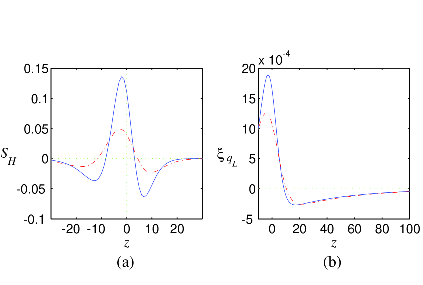
Figure 1: (a) The source for baryogenesis from the chiral classical force, eq. (167), for the parameters $\mu=100$ GeV and $m_{2}=150$ GeV and $\ell_{w}=10/T$ (solid line) and $\ell_{w}=14/T$ (dashed line). (b) The left-handed quark asymmetry $\xi_{q_{L}}$, eq. (154), for the same parameters. The distance from the center of the wall $z$, is measured in units $1/T$.

To fully specify the source term, we must also give the functional form for the spatial variation of the Higgs field condensate, since this enters the mass eigenstates $m_{\pm}$ and the CP-violating phase $\theta_{\pm}^{\prime}$ in the above formulas. Because our source is proportional to the combination $H_{1}H_{2}^{\prime}+H_{2}H_{1}^{\prime}$ of the two Higgs fields, our results are not sensitive to changes in the ratio $\tan\beta=H_{2}/H_{1}$, which is in fact known to be nearly constant for bubble walls in the MSSM—at least for generic parameter values, including those that give a strong enough phase transition. This is in marked contrast to other analyses where the source was assumed to be proportional to $H_{1}H_{2}^{\prime}-H_{2}H_{1}^{\prime}$. It thus suffices for us to use a simple kink profile

$$u(z)\equiv g\sqrt{H_{1}^{2}+H_{2}^{2}}=g\,\frac{v_{c}}{\sqrt{2}}\,\frac{1}{2}\left(1-{\tanh}\left(\frac{z}{\ell_{w}}\right)\right)$$ (168)

with $u_{1}=u\sin\beta$ and $u_{2}=u\cos\beta$. Here $\ell_{w}\sim 6-14/T$ [27, 13] is the wall width and $v_{c}$ is the value of the Higgs condensate at the critical temperature. This VEV has the usual normalization in the vacuum $v_{T=0}\simeq 246$ GeV, while the requirement for a strongly enough first order transition (to avoid washout) is $v_{c}/T_{c}>1.1$.

We display the source (167) as a function of position relative to the wall (at $z=0$) in Fig. 1(a), using the parameters values $m_{2}=150$ GeV $\mu=100$ GeV, $\delta_{\mu}\equiv\arg(m_{2}\mu)=\pi/2$ and $v_{w}=0.3$ for two different wall widths: $\ell_{w}=10/T$ and $\ell_{w}=14/T$. For the parameters left unspecified above we use the following standard reference values:

$$D_{h}=20/T\quad\Gamma_{hf}=0.013\quad\Gamma_{m}=0.007T\quad\Gamma_{+}=0.02T,\quad R={\Gamma_{-}\over\Gamma_{+}}=0.25$$

$$\ell_{w}=10/T,\quad v_{c}=120,\quad T=90,\quad\tan\beta=3.$$ (169)

In the limit that $u^{2}\ll\mu^{2},m_{2}^{2}$, the source would be a symmetric function of $z$ since it would be proportional to $(u^{2})^{\prime\prime\prime}$. However for finite $\mu$ and $m_{2}$, the actual $z$-dependent mass eigenvalues appearing in the coefficient of $(u^{2})^{\prime\prime\prime}$ depend on $u^{2}$ rather than its derivatives, hence the departure from the symmetric form. In figure 1(b) we plot the profile for left-handed quark number, $\xi_{q_{L}}$, for the same set of parameters. As expected, the spatial extent of the quark asymmetry is roughly the diffusion length of the Higgsinos, $D_{h}/v_{w}\sim 60/T$ (see the remarks below eq. (135)). For a smaller wall velocity the diffusion tail extends further, but the amplitude of $\xi_{q_{L}}$ in the tail gets smaller because then the damping has more time to suppress the chargino asymmetry.

The rates quoted in (169) are rough estimates, obtained from an approximate computation of a subset of relevant $2{\rightarrow}2$ reaction rates, and higgsino decay rates, when kinematically allowed. For example $\tilde{h}_{2}W^{3}_{\mu}{\rightarrow}\tilde{t}_{R}q_{L}$, gives

$$\sigma_{W}\simeq\frac{g^{2}y^{2}}{64\pi s}{\Bigl{(}\frac{3}{2}+{\rm ln}\frac{s}{m_{\tilde{t}_{R}}^{2}}\Bigr{)}},$$ (170)

where $s\simeq 20T^{2}$ is the center of mass energy squared and $m_{\tilde{t}_{R}}^{2}\simeq m_{U}^{2}+0.9T^{2}$ is the thermal mass of the right handed squark [37]. The soft SUSY breaking mass parameter $m_{U}^{2}$ is taken to be negative, $m^{2}_{U}\sim-60^{2}$ GeV², as indicated by the need to get a strong enough first order phase transition [12]. The rates (169) correspond to a conservative overestimate by a factor of 5 over the total averaged contribution from various scattering channels (for how to perform the thermal averages, see ref. [35]). The decay rates have a fairly strong dependence on higgsino mass $m_{\tilde{h}}\simeq\mu$. For example $\tilde{h}_{2_{L}}{\rightarrow}\tilde{t}_{R}b_{L}^{c}$ gives

$$\Gamma\simeq\frac{m_{\tilde{h}}}{16\pi}\lambda^{3/2}(1,{\textstyle{m_{b_{L}}^{2}\over m_{\tilde{h}}^{2}}},{\textstyle{m_{\tilde{t}_{R}}^{2}\over m_{\tilde{h}}^{2}}}),$$ (171)

where $\lambda(x,y,z)\equiv(x-y-z)^{2}-4yz$ and $m_{b_{L}}\simeq 0.76T$ [38]. For small $\mu\mbox{\raisebox{-2.58334pt}{~{}$\stackrel{{\scriptstyle<}}{{\sim}}$~{}}}130$ GeV, the decay channels are not open, whereas for large enough $\mu$ they dominate over the scattering contribution. However, our numerical results for $\eta_{B}$ are fairly insensitive to changes in various rates; for example decreasing $\Gamma_{+}$ by a factor of 5, appropriate for $\mu\mbox{\raisebox{-2.58334pt}{~{}$\stackrel{{\scriptstyle<}}{{\sim}}$~{}}}130$ GeV would increase $\eta_{B}$ by about 30 per cent, whereas incrasing it by a factor of 5, appropriate for $\mu\simeq 500$ GeV, would decrease $\eta_{B}$ by about 40 per cent. This scaling is somewhat weaker than the naively expected $\eta_{B}\sim 1/\sqrt{\Gamma_{+}}$ dependence, because the damping effect due to faster rates is initially being compensated by more efficient transport from the chargino sector. (We have checked that the naive scaling eventually follows for values of $\Gamma_{+}$ large enough that the transport effect has been saturated.) Nevertheless, the relative insensitivity of the results on the rates warrants our use of the rough estimates (169) in our numerical work.

6 Results

Dependence on squark spectrum. Let us first consider the dependence of $\eta_{\scriptscriptstyle B}$ on the squark spectrum. This is contained in the parameter $C(\tilde{\kappa}_{i})$, some representative values of which are given in Table 1. For certain choices of squark masses, $C(\tilde{\kappa}_{i})=0$, which reflects the approximation we made of taking the strong sphalerons to be in equilibrium; it is well known that these interactions tend to damp the baryon asymmetry if, for example, no squarks are present [39]. In these cases the baryon asymmetry is not really zero, but comes from $1/\Gamma_{ss}$ corrections which we have not computed. Ignoring such corrections, one sees the clear preference for the minimal possible number of light squark species from $C(\tilde{\kappa}_{i})$. This is fortuitous because it coincides with the need for a single, light, right-handed stop in order to get a strong phase transition. If the left-handed stops and sbottoms are also light (which, incidentally, is incompatible with the large radiative corrections needed for the Higgs mass to satisfy the experimental lower limit, as well as rho parameter constraints) the baryon asymmetry is reduced by a factor of ten. Thus, considerations both of the initial baryon production and the preservation from washout favor the “light stop scenario.”  Since the effects of the spectrum are trivial to account for in the final results, being just an overall multiplicative factor, we shall henceforth concentrate only on the most favorable scenario.

light squarks	$C(\tilde{\kappa}_{i})$
All	0
All R-chiral	0
All 3rd family	0
$\tilde{t}_{L},\;\tilde{b}_{L}$ and $\tilde{t}_{R}^{\phantom{|}}$	2/41
$\tilde{t}_{L}$ and $\tilde{t}_{R}^{\phantom{|}}$	3/16
$\tilde{t}_{R}$ and $\tilde{b}_{R}^{\phantom{|}}$	3/8
$\tilde{t}_{R}^{\phantom{|}}$ only	10/23

Table 1: Multiplicative factor $C(\tilde{\kappa}_{i})$ containing the dependence of $\eta_{\scriptscriptstyle B}$ on the squark masses for particular choices of the light squark spectrum.

Velocity dependence. The dynamics of the phase transition, even apart from CP-violating effects studied here, is a very complicated phenomenon, involving hydrodynamics of the fluid interacting with the expanding walls, and reheating effects due to the latent heat released in the transition [40]. Although the originally spherical bubbles quickly grow and reach some terminal velocity, inhomogeneities can subsequently develop. This occurs when the shock waves from the bubble expansion heat the ambient plasma and thereby reduce the latent heat released as regions of space are converted from the symmetric to the broken phase. There is a subsequent decrease of pressure driving the expansion, and depending on model parameters, may lead to significant slowing down of the walls. The process of heating by a collection of shock waves causes local variations in the temperature as well as fluid velocities, with consequent deformation of the shape and speed of the wall. These variations occur on the macroscopic length scale of the bubble radius, which is many orders of magnitude greater than the microphysical scales that have been discussed here so far. In this sense, eq. (160) gives only the local baryon number at a given position in space after the wall passes by. The presently observed asymmetry should be computed by averaging over a region which is large compared to the bubble size at the time the phase transition completes:

$$\eta_{\scriptscriptstyle B}=\frac{1}{{\rm Volume}}\int d^{\,3}{x}\,\eta_{\scriptscriptstyle B}[v_{w}(x)],$$ (172)

where $\eta_{\scriptscriptstyle B}$ is considered as a functional of the locally varying wall velocity. Only if the phase transition is very strong, so that there is a high degree of supercooling, will the reheating effects leading to inhomogeneities be small or negligible.

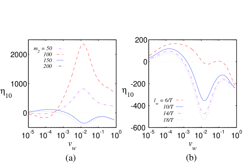
Figure 2: $\eta_{10}$ as a function of wall velocity for $\mu=100$ GeV and $\sin\delta_{\mu}=1$ for: (a) a varying gaugino mass parameter $m_{2}=50$, $100$, $150$ and $200$ GeV and: (b) for a varying wall width, $\ell_{w}=6/T$, $10/T$, $14/T$ and $18/T$.

In addition to the possibility that $v_{w}$ has spatial inhomogeneities, it is also interesting to study the dependence on $v_{w}$ simply because its value is not yet known with great certainty, although some progress has recently been made [28, 29]. Our treatment takes into account the back-reaction effect on the baryoproduction (washout by sphalerons), so our results are valid for arbitrarily small wall velocities. In Fig. 2(a) we plot $\eta_{10}\equiv\eta_{\scriptscriptstyle B}\times 10^{-10}$ as a function of $v_{w}$ for $\mu=100$ GeV and $m_{2}=50$, $100$, $150$ and $200$ GeV, and in Fig. 2(b) for four different values of the wall width $\ell_{w}$, with $\mu=100$ GeV and $m_{2}=150$ GeV.

The peak occurring at $v_{w}\simeq 0.01$ for some parameters in Fig. 2 (a), first observed in [21], is due to the contribution from the ${\cal G}_{-}$ term in (162). This is enhanced by a factor $(v_{w}+D_{h}k_{B})^{-1}$, which for the assumed parameter values peaks near $v_{w}\mbox{\raisebox{-2.58334pt}{~{}$\stackrel{{\scriptstyle<}}{{\sim}}$~{}}}\sqrt{D_{h}k_{B}}\simeq 0.01$. Because of the back-reaction, the baryon asymmetry vanishes when the wall velocity goes to zero. The peak is prominent only for the values of $m_{2}\sim\mu$ however, and the typical velocity depencence of $\eta_{10}$ is not quantitatively very large as a function of velocity. It is quite complicated however, in that for special parameter values the asymmetry can accidentally be small or zero. The crossings through zero arise as follows: for relatively large $v_{w}$ the baryon production in the diffusion tail dominates over the opposing contribution generated near the wall (see the generic form of the $\xi_{q_{L}}$ distribution in Fig. 1 (b)). For small wall velocities the length of the diffusion tail increases as $D/v_{w}$, but the amplitude of the asymmetry gets smaller due to interactions, which have more time to damp the asymmetry. Moreover, the contribution from the part of the diffusion tail extending beyond $1/k_{B}$ is cut out, because the baryon asymmetry is already relaxing due to sphaleron washout beyond that distance. As a result the contribution from the tail eventually becomes the smaller one, leading to a cancellation between the two contributions that give the net asymmetry.

While the uncertainty in $v_{w}$ at present is not necessarily the dominant one for estimating the baryon asymmetry, determining $\eta_{10}$ to high precision for a given set of chargino mass parameters would need careful hydrodynamical modelling of the bubble wall expansion. Also, even rather small fluctuations in $\eta_{B}$ can have interesting consequences elsewhere: for example they can seed the generation of large fluctuations in leptonic asymmetries in certain neutrino-oscillation models [41] with potentially large effects on nucleosynthesis.

Dependence on chargino mass parameters. The most important supersymmetric inputs directly affecting the baryon asymmetry are the chargino mass parameters $m_{2}$ and $\mu$, and the CP-violating phase $\delta_{\mu}\equiv{\rm arg}(m_{2}\mu)$. In Fig. 4a and 4b we plot the contours of constant $|\delta_{\mu}|$ giving the desired baryon asymmetry $\eta_{\scriptscriptstyle B}=3\times 10^{-10}$ [42] in the $(m_{2},\mu)$ plane. The baryoproduction is most efficient for small masses, $m_{2},\mu\mbox{\raisebox{-2.58334pt}{~{}$\stackrel{{\scriptstyle<}}{{\sim}}$~{}}}100$ GeV, but baryons can still be copiously produced for $|m_{2}|$ and $|\mu|\sim$ 500 GeV and higher. In the best cases, a large enough baryon asymmetry can be produced even with a very small explicit CP-violating angle of order a few $\times 10^{-3}$, comfortably within the constraints coming from electric dipole moment searches [43].

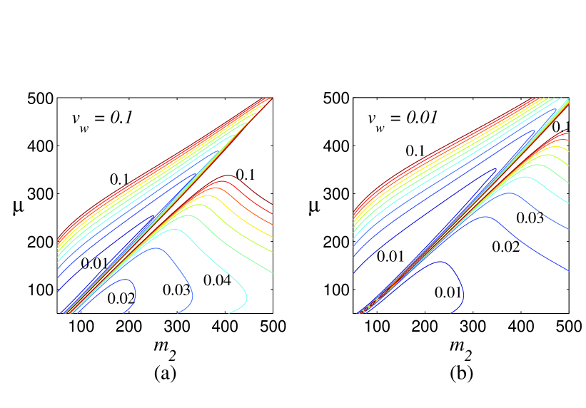
Figure 3: Contours of constant CP-violating phase $\delta_{\mu}$, corresponding to baryon asymmetry $\eta_{\scriptscriptstyle B}=3\times 10^{-10}$ for (a) $v_{w}=0.1$ and (b) $v_{w}=0.01$. Mass units are GeV.

7 Conclusions and outlook

We have presented a detailed analysis of electroweak baryogenesis in the minimal supersymmetric standard model (MSSM) using the classical force mechanism (CFM). We argued that the dominant baryogenesis source in the MSSM arises from the chargino sector. We also commented on a recent controversy regarding the parametric form of the source appearing in the diffusion equations. The resolution is that all different formalisms agree with the parametric form; however previous authors neglected the particular source considered here for the linear combination of Higgsinos $H_{1}+H_{2}$, on the grounds that it is suppressed by the top (s)quark Yukawa interactions. We have shown that this suppression is quite modest, a factor of order unity, which is much milder than the intrinsic suppression suffered by the competing source $H_{1}-H_{2}$, due to the near constancy of the ratio $H_{1}/H_{2}$ throughout the bubble wall [27, 13].

Our present work differs in several ways from our earlier published results using the CFM. First we have presented a treatment in terms of the physical, kinetic variables characterizing the WKB states rather than in terms of canonical variables, which are gauge dependent, and in terms of which the recovery of a gauge independent physical result is not always transparent. While this is mainly a matter of (considerable!) convenience, there is also a slight physical difference in our results due to a slightly different form for equilibrium ansatz corresponding to each parametrization (see appendix B). We noted that a definitive determination of the correct form will have to await the outcome of a more fundamental computation, as will the correct treatment of ‘spontaneous’ baryogenesis, which rely completely on the relevant form of the collision integral. Much more importantly to quantitative changes in our results is that in our treatment in [19] we misidentified the sign of the hypercharge of one of the Higgsino states. This prevented us from realizing that the top Yukawa interactions tend to damp the appropriate combination of Higgsino currents, $H_{1}+H_{2}$. Here we developed a new set of diffusion equations where this effect is treated correctly. Thirdly, here we have considered several different choices for which flavors of squarks are light compared to the temperature, and found that the one adopted in [19] (all squarks light) is among the less favoured possiblities for baryogenesis, because of strong sphaleron suppression.

We have given a complete derivation of the CFM formalism, starting from the basic assumption that the plasma is adequately described by a collection of WKB-quasiparticle states in the vicinity of a varying background Higgs field. We derived the dispersion relations for squarks and charginos, and showed how to identify the appropriate kinetic momentum variable, the physical group velocity, and the force (see also [22]). We pointed out that the force term for the current combination $H_{1}-H_{2}$, obtained in a recent publication [23], is absent in physical variables and hence this current is not sourced in the CFM. This is a very sensible result, because the term in question can always be removed by a canonical transformation, or equivalently, a field redefinition. We also derived the diffusion equations and the source terms appearing in them starting from the semiclassical Boltzmann equations for the quasiparticle states.

We have studied the baryon production efficiency in the MSSM as a function of the parameters in the chargino mass matrix, the wall width and the wall velocity. The dependence on wall velocity is rather complicated, and intertwined with the dependence on the chargino mass parameters; the generated asymmetry generically changes sign as a function of $v_{w}$, but the value of $v_{w}$ where this crossing takes place, and the the functional form of $\eta_{B}(v_{w})$, are quite dependent on mass parameters. However, for large regions of parameters an asymmetry $\eta_{10}\equiv 10^{10}\eta_{B}$ of the order of several hundred could be created, implying that a CP-violating angle of $\arg(m_{2}\mu)\simeq 10^{-2}$, and in best cases even $\arg(m_{2}\mu)\simeq$ a few$\times 10^{-3}$, suffices for producing the observed asymmetry of $\eta_{10}\sim 3$ [42]. Such small phases are consistent with the present limits from the neutron and electron dipole moment constraints [43].

We finally emphasize that our formalism disagrees in detail with various other methods of computing the source in the diffusion equations. This is particularly significant with regard to references [25, 15, 26, 18], which all claim to be valid in the thick wall regime, where our method was designed to work. This is troubling, because one expects that different methods should agree when the same physical limits are taken. In particular, we have shown that classical force mechanism does not give rise to a source of the parametric form $\sim H_{1}^{\prime}H_{2}-H_{1}H_{2}^{\prime}$, found by references [25, 15, 26, 18, 23] for both squarks and charginos. We do not know a definite solution to this problem, but a possible origin for the discrepancy could be that the methods [25, 15, 26, 18] perform an expansion in the mass, or the vacuum expectation value, divided by temperature (the mass insertion expansion [26]), before taking the gradient expansion. In the WKB approach on the other hand the background is treated in a mean field approximation and one performs the gradient expansion around this classical background. In other words, in the WKB-picture the mass insertion expansion has been resummed to infinite order before the gradient limit is considered. While one can formally expand the CFM-source resulting from a WKB-analysis in mass over temperature, one should in general not expect that taking these two limits is commutative. In particular, quantum reflection is completely absent in the WKB approximation, but is certainly present in the mass insertion expansion. The issue of how to properly account for both the semiclassical and the quantum effects, or to interpolate between them, is certainly worth further study, and some published results from a work aiming to a derivation of appropriate semiclassical Boltzmann equations from first principles can be found in references [33, 32].

Appendix A: Collision Terms in Linear Expansion

We show here how the collision integral on the r.h.s. of the Boltzmann equation gives rise to the terms damping the perturbations from equilibrium. For illustration, let us consider a two body process with ingoing WKB states $i$ with four momenta $p_{i}$ (with $p_{i1}$ corresponding to the distribution on the l.h.s. of the Boltzmann equation) and outgoing WKB states $f$ with four momenta $p_{f}$:

$$C[f_{j}]={1\over 2E_{i1}}\int_{p_{i2},p_{f}}|{\cal M}|^{2}(2\pi)^{4}{\delta\!\!\!^{-}}^{4}\Bigl{(}\sum_{l}\hat{p}_{l}\Bigr{)}{\cal P}[f_{j}]$$ (173)

where $|{\cal M}|^{2}$ is the matrix element calculated between the WKB states, to first order in derivatives of the background, $\int_{p}$ means $\int{\rm d}^{3}p/2E(2\pi)^{3}$ and the statistical factor ${\cal P}[f_{j}]$ is given by

$${\cal P}[f_{i}]=f_{i1}f_{i2}(1\mp f_{f1})(1\mp f_{f2})-f_{f1}f_{f2}(1\mp f_{i1})(1\mp f_{i2}).$$ (174)

We only attempt to compute the collision integrals to the zeroth order accuracy in gradients, so that the integral measures and $\delta$-functions are the same as in the usual flat space-time considerations. Most part of the derivation consists of manipulating the statistical factor ${\cal P}[f_{i}]$. Inserting the ansatz (87) to (174) and expanding to the first order in $\delta\!f$ one gets

$${\cal P}[f_{i}(\mu_{i})+\delta\!f_{i}]\simeq{\cal P}[f_{i}(\mu_{i})]+f^{0}_{i1}f^{0}_{i2}f^{0}_{f1}f^{0}_{f2}e^{\beta(E_{i1}+E_{i2})}\left(\frac{\delta\!f_{i1}}{f^{0}_{i1}}+\frac{\delta\!f_{i2}}{f^{0}_{i2}}-\frac{\delta\!f_{f1}}{f^{0}_{f1}}-\frac{\delta\!f_{f2}}{f^{0}_{f2}}\right),$$ (175)

where $f_{i}(\mu_{i})$’s are the distributions given by the first term in the ansatz (87) and $f^{0}_{j}$’s are the unperturbed distribution functions. ${\cal P}[f_{i}(\mu_{i})]$ is nonzero only for inelastic scatterings, whereas all reaction channels create nonvanishing collision terms proportional to $\delta\!f_{j}$; let us consider these terms first.

The entire collision integral corresponding to $\delta\!f_{j}$-terms in (175)can be written as

$$C[\delta\!f_{l}] \simeq \delta\!f_{i1}(p_{1})\Gamma(p_{i1})+f^{0}(p_{i1})\int_{p_{i2}}\delta\!f_{i2}(p_{i2})a(p_{i1},p_{i2})$$ (176)

$$\phantom{Hannatytton}-\sum_{n}\int_{p_{fn}}\delta\!f^{0}_{fn}(p_{fn})G_{fn}(p_{i1},p_{fn})$$

$$\equiv \delta\!f_{i1}(p_{1})\Gamma(p_{i1})-\delta\!F(p_{i1})$$

The abbreviated notation here is used to highlight the fact that only the first term is directly proportional to $\delta\!f_{i1}(p_{i1})$, whereas all the others contain smeared integrals over $\delta\!f_{j}$-distributions; the exact forms of the functions $a(p,k)$ and $G_{i}(p,k)$ are not relevant for us. $\Gamma(p_{i1})$ on the other hand is the usual thermally averaged interaction rate, which, neglecting the Pauli-blocking factors, is given by

$$\Gamma(p_{i1})=\int\frac{{\rm d}^{3}p_{i2}}{(2\pi)^{3}}f^{0}_{i2}(p_{i2})(v_{\rm rel}\sigma_{i{\rightarrow}j}).$$ (177)

where

$$(v_{\rm rel}\sigma_{i{\rightarrow}j})\equiv\frac{1}{4E_{i1}E_{i2}}\int_{p_{f}}(2\pi)^{4}\delta^{4}(\sum_{l}p_{l})|{\cal M}|^{2}$$ (178)

is the invariant cross section for the process $i{\rightarrow}f$ multiplied by the invariant flux (see for example [30]).

The $\delta\!f\;\Gamma$-term in (176) clearly causes damping away of kinetic fluctuations, with a momentum dependent relaxation scale given by the inverse of the rate (177). The “noise term” $\delta\!F$ physically represents the process of further thermal redistribution of the states which goes on alongside the relaxation of $\delta\!f_{i}$ to zero. Thes are random processes which occasionally oppose the relaxation process. However, while the integrated over $p_{i1}$ moments of $\delta\!F(p_{i1})$ are comparable to the moments of the first term, their naive inclusion to the moment equations would be incorrect, since kinetic relaxation depends sensitively on the shape of the entire distribution function. For example, the condition ${\left\langle(p_{i1}/E_{i0})(\delta\!f\Gamma-\delta\!F)\right\rangle}=0$ would lead to vanishing of the (kinetic) relaxation term for the velocity perturbation in moment equations, whereas in reality the kinetic relaxation process is halted only if the collision term (176) vanishes identically for all momenta. The effect of the noise terms is further reduced by the fact that in all elastic channels adding the scatterings from particles and antiparticles tend to cancel the noise part, while the contributions to the relaxation terms are equal and add. In the diffusion approximation then, the first moments of the part of the collision term containing $\delta\!f_{j}$’s are given by

$${\left\langle C[\delta\!f_{j}]\right\rangle} \simeq 0$$

$${\left\langle v_{p_{z}}C[\delta\!f_{j}]\right\rangle} \simeq {\left\langle v_{p_{z}}\delta\!f_{i1}(p_{z})\right\rangle}\bar{\Gamma},$$ (179)

where the average ${\left\langle\cdot\right\rangle}$ is as defined in equation (96). In the case of first moment we have also assumed that $\Gamma(p)$ has only a weak momentum dependence so that it can be replaced by its thermal average $\bar{\Gamma}$. This is of course the place where we implicitly truncate our momentum expansion to the first two terms, and it should be a very good approximation. Adding up the contributions from all possible channels, one obtains the result (101).

Let us next consider the ${\cal P}[f(\mu_{j})]$-part of the statistical factor (175). Expanding to the first order in $\mu_{j}$’s one finds

$${\cal P}[f(\mu_{j})]\simeq-f^{0}_{i1}f^{0}_{i2}(\xi_{i1}+\xi_{i2}-\xi_{f1}-\xi_{f2}),$$ (180)

where $\xi\equiv\mu/T$ and we also neglected the Pauli blocking factors in the final states. This expression obviously vanishes for the elastic channels, whereas for inelastic channels it gives the contribution

$$C[\mu_{j}]\simeq f^{0}_{i1}(p_{i1})\Gamma_{i}(p_{i1})\sum_{j}\xi_{j}$$ (181)

where $\Gamma_{i}(p_{i1})$ is an expression analogous to (177) and $\sum_{j}\xi_{j}$ is the signed sum over the chemical potentials appearing in (180) such that the term $\xi_{i1}$ has a positive sign. The first moments of the inelastic collision term in (181) then are

$${\left\langle C[\mu_{j}]\right\rangle} \simeq \bar{\Gamma}_{i}\sum_{j}\xi_{j}$$

$${\left\langle v_{p_{z}}C[\mu_{j}]\right\rangle} \simeq 0$$ (182)

where

$$\bar{\Gamma}_{i}\equiv\int_{p_{i1}}f^{0}_{i1}\Gamma_{i}(p_{i1})/N_{i1}$$ (183)

with $N_{i1}\equiv\int{\rm d}^{3}pf_{i0}^{\prime}$ (see equation (96)). Adding up all inelastic channels affecting a given species $i$, one arrives to the equation (100).

Appendix B: Equilibrium ansatz in canonical variables

Gauge invariance. In previous treatments [7, 19] an ansatz different from (86) was adapted for the local equilibrium function:

$$\tilde{f}(p_{c},x)={1\over e^{\beta[\gamma_{w}(\omega+v_{w}p_{c})-\tilde{\mu}(x)]}\pm 1}+\delta\!\tilde{f}(p,x),$$ (184)

where $p_{c}$ is the canonical momentum. A technical problem with the canonical variables is that both $p_{c}$ and $\tilde{\mu}$ are phase reparametrization, or “gauge” variant quantities. This can be seen by observing that any physical quantity (e.g. local number density) is obtained integrating over the momenta. The integration measure $d^{3}p_{c}$ is unchanged by gauge transformation $p_{c}\rightarrow p_{c}+\alpha_{\scriptscriptstyle CP}$, so that a system with fixed number density is described by a different value of $\tilde{\mu}$ in two different gauges.

In the previous treatments [7] and [19] equations for physically meaningful quantities were recovered using the condition that the system be unperturbed from equilibrium far in front of the wall (at $z\rightarrow\infty$) i.e.

$$\int d^{3}p_{\infty}\tilde{f}=\int d^{3}p_{\infty}\frac{1}{e^{\beta[\gamma_{w}(\omega+v_{w}p_{\infty})-\mu_{\rm phys}]}\pm 1}\qquad\mu_{\rm phys}\rightarrow 0\quad{\rm as}\quad z\rightarrow\infty$$ (185)

where $p_{\infty}$ is the physical momentum at infinity. For the case of a fermion with complex mass discussed in section 2, Eqns. (17) and (18) give

$$p_{\infty}=p_{c,\infty}+s_{\scriptscriptstyle CP}\frac{s\theta^{\prime}}{2}-\alpha_{\scriptscriptstyle CP}$$ (186)

(since $m\rightarrow 0$), where $\alpha_{\scriptscriptstyle CP}\equiv\alpha^{\prime}+s_{\scriptscriptstyle CP}\theta^{\prime}/2$ in the leftchiral sector for example. One then identifies the physical chemical potential as

$$\mu_{\rm phys}=\tilde{\mu}+v_{w}\gamma_{w}(s_{\scriptscriptstyle CP}\frac{s\theta^{\prime}}{2}-\alpha_{\scriptscriptstyle CP}).$$ (187)

The equations are then most conveniently rewritten in terms of $\mu_{\rm phys}$ and $p_{\infty}$, and solved with with the boundary condition $\mu_{\rm phys}=0$ at $+\infty$. Note that in both [7] and [19] a specific gauge was chosen, which can be read off from the dispersion relations adapted as $\alpha_{\scriptscriptstyle CP}=0$ in [7], and $\alpha_{\scriptscriptstyle CP}=s_{\scriptscriptstyle CP}\frac{s\theta^{\prime}}{2}$ in [19]. While in the former case a transformation from the original canonical variables had to be performed (cf. section 4, page 2962 in [7]), the implicit gauge choice of [19] required no such transformation, since $\mu_{\rm phys}=\tilde{\mu}$ in this gauge. Note in particular that the terms proportional to the linear combination of scalar fields $H_{1}^{\prime}H_{2}-H_{2}^{\prime}H_{1}$ appearing in canonical momenta (43), (64) and (69), can entirely be absorbed into the redefinition of $\mu_{\rm phys}$, so they will not provide new sources even when treating the problem using the canonical momentum.

Comparision of the ansätze. Making use of (20) and the dispersion relation (19) one can show that the canonical and kinetic momenta are, to linear order in $\theta^{\prime}$, related by

$$p_{z}(1-s_{\scriptscriptstyle CP}\frac{s\theta^{\prime}}{2\tilde{\omega}})=p_{c}-\alpha_{\scriptscriptstyle CP},$$ (188)

where $\tilde{\omega}\equiv\sqrt{\omega^{2}-p^{2}_{||}}$. In kinetic variables the ansatz (185) may then be written as

$$\tilde{f}(p,x)=\frac{1}{e^{\beta[\gamma_{w}(\omega+v_{w}p)-\mu_{\rm phys}]}\pm 1}+\delta\!\tilde{f}(p,x)+\beta v_{w}\gamma_{w}s_{\scriptscriptstyle CP}\frac{s\theta^{\prime}}{2}\frac{\tilde{\omega}-p}{\tilde{\omega}}f^{\prime},$$ (189)

where $f^{\prime}=(1/e^{x}\pm 1)^{\prime}$ ($x=\beta\omega$). One can thus identify the physical chemical potential $\mu_{\rm phys}$ in the canonical variables with the chemical potential for our physical WKB-quasiparticles appearing in the ansatz (87). The chemical potentials in (87) and (184) are thus only separated by an unphysical gauge-transform. The distributions differ however, by a term that cannot be transformed away: to make (184) completely agree with (87), one should have

$$\delta\!\tilde{f}=\delta\!f-\beta v_{w}\gamma_{w}s_{\scriptscriptstyle CP}\frac{s\theta^{\prime}}{2}\frac{\tilde{\omega}-p}{\tilde{\omega}}f^{\prime}.$$ (190)

The latter term does not vanish in equilibrium however, so the two ansätze do correspond to two physically different equilibrium conditions. The difference is only nonzero in the region of the wall however, as it vanishes when $|m|{\rightarrow}0$. Including this term in our Boltzmann equations would contribute to source term, making it equal to the one used in [19].

It is clear that the difference between ansätze corresponds to which energy momentum - canonical or kinetic - is the appropriate one to take as that conserved in the local interactions between particle states modelled there. We have argued in the main text that the kinetic momentum has the more direct physical interpretation, and this argument is backed up by results from a more sophisticated treatment [32, 33]. However, a complete derivation of the transport equations using the formalism of [32, 33] will be needed to settle the issue unambiguously, while in practice the numerical results are not particularily sensitive to the difference.

References

- [1]
-
[2]
A. Cohen, D. Kaplan, and A. Nelson,
Annual Review of Nuclear and Particle Science
43 (1994) 27;
V.A. Rubakov and M.E. Shaposhnikov, Usp. Fiz. Nauk 166 (1996) 493; Phys. Usp. 39 (1996) 461. -
[3]
M.E. Shaposhnikov, Jetp. Lett. 44 (1986) 465;
Nucl. Phys. B287 (1987) 757; Nucl. Phys. B299 (1988) 797;
G. Farrar and M. Shaposhnikov, Phys Rev. Lett. 70 (1993) 2833, erratum ibid. 71 (1993) 210; Phys. Rev. D50 (1993) 774
M.B. Gavela, P. Hernandez, J. Orloff and O. Pene, Mod. Phys. Lett. A9 (1994) 795; Nucl. Phys. B430 (1994) 345. - [4] M. Joyce, Phys. Rev. D55 (1997) 1875; M. Joyce and T. Prokopec, Phys. Rev. D57 (1998) 6022.
- [5] K. Kajantie, M. Laine, K. Rummukainen and M.E. Shaposhnikov, Nucl. Phys. B466 (1996) 189.
- [6] G.W. Anderson and L.J. Hall, Phys. Rev. D45 (1992) 2685; N. Turok and J. Zadrozny, Nucl. Phys. B369 (1992) 792.
- [7] M. Joyce, T. Prokopec and N. Turok, Phys. Lett. B338 (1994) 269; Phys Rev. Lett. 75 (1995) 1695; ibid. 75 (1995) 3375 (Erratum); Phys. Rev. D53 (1996) 2958.
- [8] M. Joyce, T. Prokopec and N. Turok, Phys. Rev. D53 (1996) 2930.
- [9] J. Cline, K. Kainulainen and A. Vischer, Phys. Rev. D54 (1996) 2451.
- [10] J.R. Espinosa, M. Quiros and F. Zwirner, Phys. Lett. B307 (1993) 106; A. Brignole, J.R. Espinosa, M. Quiros and F. Zwirner, Phys. Lett. B324 (1994) 181.
- [11] M. Carena, M. Quiros and C. E. Wagner, Phys. Lett. B380 (1996) 81; Nucl. Phys. B524 (1998) 3; J.M. Cline and K. Kainulainen, Nucl. Phys. B482 (1996) 73; Nucl. Phys. B510 (1998) 88; M. Laine, Nucl. Phys. B481 (1996) 43; M. Losada, Phys. Rev. D56 (1997) 2893; G. Farrar and M. Losada, Phys. Lett. B406 (1997) 60. J.R. Espinosa, Nucl. Phys. B475 (1996) 273; B. de Carlos and J. R. Espinosa, Nucl. Phys. B503 (1997) 24; D. Bodeker, P. John, M. Laine and M.G. Schmidt, Nucl. Phys. B497 (1997) 387.
- [12] M. Laine and K. Rummukainen,Phys Rev. Lett. 80 (1998) 5259; Nucl. Phys. B535 (1998) 423.
- [13] J. M. Cline and G. D. Moore, Phys Rev. Lett. 81 (1998) 3315.
- [14] A. G. Cohen and A. E. Nelson, Phys. Lett. B297, 111 (1992) [hep-ph/9209245].
- [15] P. Huet and A.E. Nelson, Phys. Rev. D53 (1996) 4578.
- [16] A.G. Cohen, D.B. Kaplan and A.E. Nelson, Phys. Lett. B336 (1994) 41.
- [17] M. Aoki, N. Oshimo and A. Sugamoto, Prog. Theor. Phys. 98 (1997) 1179; Prog. Theor. Phys. 98 (1997) 1325.
- [18] M. Carena, M. Quiros, A. Riotto, I. Vilja and C.E.M. Wagner, Nucl. Phys. B503 (1997) 387.
- [19] J.M. Cline M. Joyce and K. Kainulainen, Phys. Lett. B417 (1998) 79; Phys. Lett. B448 (1999) 321 (Erratum).
- [20] N. Rius and V. Sanz, Nucl. Phys. B570 (2000) 155.
- [21] J.M. Cline and K. Kainulainen, hep-ph/0002272.
- [22] K. Kainulainen, hep-ph/0002273.
- [23] S.J. Huber, M.G. Schmidt, hep-ph/0003122.
- [24] A.G. Cohen, D.B. Kaplan and A.E. Nelson, Phys. Lett. B199 (1987) 257; Nucl. Phys. B308 (1988) 913.
- [25] P. Huet and E. Sather, Phys. Rev. D51 (1995) 379.
- [26] A. Riotto, Nucl. Phys. B518 (1998) 339.
- [27] J. M. Moreno, M. Quiros and M. Seco, Nucl. Phys. B526 (1998) 489.
- [28] G. Moore, JHEP 0003:006,2000.
- [29] P. John and M.G. Schmidt, hep-ph/0002050.
- [30] A. Dolgov and K. Kainulainen, Nucl. Phys. B402 (1993) 349.
- [31] G.D. Moore and T. Prokopec, Phys. Rev. D52 (1995) 7182.
- [32] M. Joyce, K. Kainulainen and T. Prokopec, hep-ph/0002239.
- [33] M. Joyce, K. Kainulainen and T. Prokopec, Phys. Lett. B468 (1999) 128; Phys. Lett. B474 (2000) 402.
- [34] G.D. Moore and K. Rummukainen. hep-ph/9906259.
- [35] J.M. Cline, K. Kainulainen and K.A. Olive, Phys Rev. Lett. 71 (1993) 2372; Phys. Rev. D49 (1994) 6394.
- [36] M. Abramovitz and A. Stegun, Handbook of mathematical functions, Dover 1970.
- [37] D. Comelli, J.R. Espinosa, Phys. Rev. D55 (1997) 6253.
- [38] S. Davidson, K. Kainulainen and K.A. Olive, Phys. Lett. B335 (1994) 339.
- [39] G.F. Giudice and M. Shaposnikov, Phys. Lett. B326 (1994) 118.
- [40] A.F. Heckler, Phys. Rev. D51 (1995) 405; H. Kurki-Suonio and M. Laine, Phys Rev. Lett. 77 (1996) 3951.
- [41] X. Shi and G.M. Fuller, Phys Rev. Lett. 83 (1999) 3120; K. Enqvist, K. Kainulainen and A. Sorri, Phys. Lett. B464 (1999) 199; P. Di Bari hep-ph/9911214.
- [42] B.D. Fields, K. Kainulainen, K.A. Olive, and D. Thomas, New Astronomy 1 (77) 1996.
- [43] P.G. Harris et al., Phys Rev. Lett. 82 (1999) 904.