Vibrating the $QCD$ string

Abstract

The large-distance behaviour of the adiabatic hybrid potentials is studied in the framework of the QCD string model. The calculated spectra are shown to be the result of interplay between potential-type longitudinal and string-type transverse vibrations.

General arguments from QCD and lattice data tell that the theory, even quenched in quarks, possesses nontrivial spectrum, so that effective degrees of freedom for constituent glue should be introduced to describe QCD in the nonperturbative region. As far as we know the possibility for mesons with gluonic lump to exist was first considered in [1] in 1976. Modern wisdom tells that the area law asymptotics for the Wilson loop implies a kind of string to be developed between quark and antiquark at large distances, and it is natural to identify the $q\bar{q}$ system connected by the string in its ground state with conventional $q\bar{q}$ meson, while the string vibrations are responsible for gluonic (hybrid) excitations. This picture, though physically appealing, does not follow directly from the QCD, and one relies upon models to describe these excitations. There are two main ideas on how to construct such models. One is to consider point-like gluons confined by some potential-type force [2, 3], and another is to introduce string phonons [4].

In principle the best way to discriminate between these two possibilities is to compare predictions with experimental data on hybrid mesons. Indeed, there is a lot of indications that hybrid mesons are already found, but the conclusive evidences have never been presented, nor have alternative explanations been completely excluded [5].

On the other hand, lattice calculations are now accurate enough to provide reliable data on the properties of soft glue and to check the model predictions. In this regard recent measurements [6] of adiabatic hybrid potentials are of particular interest. These simulations measure the spectrum of glue in the presence of static quark and antiquark separated by some distance $R$. Not only these potentials enter heavy hybrid mass estimations in the Born-Oppenheimer approximation. The large $R$ limit is important per se, as the formation of confining string is expected at large distances, and direct measurements of string fluctuations become available. It is our purpose to investigate the large-distance behaviour of adiabatic potentials in order to establish what kind of the effective string degrees of freedom are excited at large distances.

We perform these studies in the framework of the QCD string model. This model deals with quarks and point-like gluons propagating in the confining QCD vacuum, and is based on Vacuum Background Correlators method [7]. The QCD string model was successfully applied to conventional mesons [8], hybrids [9, 10, 7], glueballs [11] and gluelump (gluon bound to the static adjoint source) [12].

The QCD string model for gluons is derived from the perturbation theory in the nonperturbative background, developed in [13]. This formalism allows to introduce constituent (valence) gluons as perturbations at the confining background. The latter is given by the set of gauge-invariant field strength correlators responsible for the area law. The main feature of this approach is that, in contrast to the above-mentioned models, here one is able to distingiush clearly between confining gluonic field configurations and confined valence gluons.

The starting point is the Green function for the gluon propagating in the given background field $B_{\mu}$ [13]:

$$G_{\mu\nu}(x,y)=(D^{2}(B)\delta_{\mu\nu}+2igF_{\mu\nu}(B))^{-1},$$ (1)

where covariant derivative $D_{\lambda}^{ca}(B)$ is

$$D_{\lambda}^{ca}(B)=\delta_{ca}\partial_{\lambda}+gf^{cba}B^{b}_{\lambda}.$$ (2)

The term proportional to $F_{\mu\nu}(B)$ is responsible for the gluon spin interaction; in these first studies we neglect it, as it can be treated as perturbation [11, 12]. The next step is to use Feynman-Schwinger representation for the quark-antiquark-gluon Green function [10], which is reduced in the case of static quark and antiquark to the form

$$G(x_{g},y_{g})=\int^{\infty}_{0}ds\int Dz_{g}\exp(-K_{g})\langle{\cal W}\rangle_{B},$$ (3)

where $K_{g}=\frac{1}{4}\int^{s}_{0}\dot{z}^{2}_{g}(\tau)d\tau$, and all the dependence on the vacuum gluonic field $B_{\mu}$ is contained in the Wilson loop

$${\cal W}=\mathrm{Sp}(\lambda_{a}\Phi_{q}\lambda_{b}\Phi_{\bar{q}})\Phi^{ab}_{\Gamma_{g}}(y_{g},x_{g}).$$ (4)

Here $\Phi_{q}$ and $\Phi_{\bar{q}}$ are parallel transporters

$$\Phi_{q}=P\exp ig\int^{x_{q}}_{y_{q}}B_{\mu}(z_{q})dz_{q\mu},~{}~{}\Phi_{\bar{q}}=P\exp ig\int^{y_{\bar{q}}}_{x_{\bar{q}}}B_{\mu}(z_{\bar{q}})dz_{\bar{q}\mu}$$ (5)

with integration in (5) along the classical trajectories $z_{q\mu}=(\tau,\frac{\mbox{\boldmath${\rm R}$}}{2})$ and $z_{\bar{q}\mu}=(\tau,-\frac{\mbox{\boldmath${\rm R}$}}{2})$ of static quark and antiquark, $P$ means path ordering, and

$$\Phi^{ab}_{\Gamma_{g}}(y_{g},x_{g})=(P\exp ig\int_{\Gamma_{g}}B_{\mu}(z_{g})dz_{g\mu})^{ab},$$ (6)

$a,b$ are adjoint colour indices, $\lambda_{a}$ are Gell-Mann matrices and the contour $\Gamma_{g}$ runs over the gluon trajectory $z_{g}$.

The main assumption of the QCD string model is the minimal area law for the Wilson loop average, which yields for the configuration (4) the form [10]

$$\langle{\cal W}\rangle_{B}=\frac{N_{c}^{2}-1}{2}\exp(-\sigma(S_{1}+S_{2})),$$ (7)

where $S_{1}$ and $S_{2}$ are the minimal areas inside the contours formed by quark and gluon and antiquark and gluon trajectories correspondingly, and $\sigma$ is the string tension.

With the form (7) for $\langle{\cal W}\rangle_{B}$ the action of the system can be immediately read out of the representation (3):

$$A=\int^{T}_{0}d\tau\left\{-\frac{\mu}{2}+\frac{\mu\dot{r}^{2}}{2}-\sigma\int^{1}_{0}d\beta_{1}\sqrt{(\dot{w}_{1}w_{1}^{\prime})^{2}-\dot{w}_{1}^{2}w^{{}^{\prime}2}_{1}}-\right.$$

$$\left.-\sigma\int^{1}_{0}d\beta_{2}\sqrt{(\dot{w}_{2}w_{2}^{\prime})^{2}-\dot{w}_{2}^{2}w^{{}^{\prime}2}_{2}}\right\},$$ (8)

where the minimal surface $S_{1}$ and $S_{2}$ are parametrized by the coordinates $w_{i\mu}(\tau,\beta_{i}),~{}i=1,2,~{}\dot{w}_{i\mu}=\frac{\partial w_{i\mu}}{\partial\tau},~{}w^{\prime}_{i\mu}=\frac{\partial w_{i\mu}}{\partial\beta_{i}}.$

In what follows the straight-line ansatz is chosen for the minimal surface:

$$w_{io}=\tau,~{}~{}~{}\mbox{\boldmath${\rm w}$}_{1,2}=\pm(1-\beta)\frac{\mbox{\boldmath${\rm R}$}}{2}+\beta\mbox{\boldmath${\rm r}$}.$$ (9)

The quantity $\mu=\mu(\tau)$ in the expression (8) for the action is the so-called einbein field [14]; here one is forced to introduce it, as it is the only way to obtain meaningful dynamics for the massless particle. Moreover, we introduce another set of einbein fields, $\nu_{i}=\nu_{i}(\tau,\beta_{i})$ to get rid of Nambu-Goto square roots in (8) [8]. The resulting Lagrangian takes the form

$$L=-\frac{\mu}{2}+\frac{\mu\dot{r}^{2}}{2}-\int^{1}_{0}d\beta_{1}\frac{\sigma^{2}r^{2}_{1}}{2\nu_{1}}-\int^{1}_{0}d\beta_{1}\frac{\nu_{1}}{2}(1-\beta_{1}^{2}l_{1}^{2})-$$

$$-\int^{1}_{0}d\beta_{2}\frac{\sigma^{2}r^{2}_{2}}{2\nu_{2}}-\int^{1}_{0}d\beta_{2}\frac{\nu_{2}}{2}(1-\beta_{2}^{2}l_{2}^{2}),$$

$$l^{2}_{1,2}=\dot{r}^{2}-\frac{1}{r^{2}_{1,2}}(\mbox{\boldmath${\rm r}$}_{1,2}\dot{\mbox{\boldmath${\rm r}$}})^{2},~{}~{}\mbox{\boldmath${\rm r}$}_{1,2}=\mbox{\boldmath${\rm r}$}\pm\frac{\mbox{\boldmath${\rm R}$}}{2}.$$ (10)

It is clear from Eq.(10) that the einbein field $\mu$ can be treated as the kinetic energy of the constituent gluon, and the einbeins $\nu_{i}(\tau,\beta_{i})$ describe the energy density distribution along the string. These quantities are not introduced by hand, but are calculated in the presented formalism. Indeed, as no time derivatives of the einbeins enter the Lagrangian (10), it describes the constrained system, with the equations of motion

$$\frac{\partial L}{\partial\mu}=0,~{}~{}\frac{\delta L}{\delta\nu_{i}(\beta_{i})}=0$$ (11)

playing the role of second-class constraints.

Now one obtains the Hamiltonian $H=\mbox{\boldmath${\rm p}$}\dot{\mbox{\boldmath${\rm r}$}}-L$ with the result

$$H=H_{0}+\frac{\mu}{2}+\int^{1}_{0}d\beta_{1}\frac{\sigma^{2}r^{2}_{1}}{2\nu_{1}}+\int^{1}_{0}d\beta_{2}\frac{\sigma^{2}r^{2}_{2}}{2\nu_{2}}+\int^{1}_{0}d\beta_{1}\frac{\nu_{1}}{2}+\int^{1}_{0}d\beta_{2}\frac{\nu_{2}}{2},$$ (12)

$$H_{0}=\frac{p^{2}}{2(\mu+J_{1}+J_{2})}+$$

$$\frac{1}{2\Delta(\mu+J_{1}+J_{2})}\left\{\frac{(\mbox{\boldmath${\rm p}$}\mbox{\boldmath${\rm r}$}_{1})^{2}}{r^{2}_{1}}J_{1}(\mu+J_{1})+\frac{(\mbox{\boldmath${\rm p}$}\mbox{\boldmath${\rm r}$}_{2})^{2}}{r^{2}_{2}}J_{2}(\mu+J_{2})+\right.$$

$$\left.\frac{2J_{1}J_{2}}{r^{2}_{1}r^{2}_{2}}(\mbox{\boldmath${\rm r}$}_{1}\mbox{\boldmath${\rm r}$}_{2})(\mbox{\boldmath${\rm p}$}\mbox{\boldmath${\rm r}$}_{1})(\mbox{\boldmath${\rm p}$}\mbox{\boldmath${\rm r}$}_{2})\right\}$$ (13)

$$\Delta=(\mu+J_{1})(\mu+J_{2})-J_{1}J_{2}\frac{(\mbox{\boldmath${\rm r}$}_{1}\mbox{\boldmath${\rm r}$}_{2})^{2}}{r^{2}_{1}r^{2}_{2}},~{}~{}J_{i}=\int^{1}_{0}d\beta_{i}\beta_{i}^{2}\nu_{i}(\beta_{i}),~{}~{}i=1,2.$$

As we deal with the constrained system, the extra variables $\mu$ and $\nu_{1,2}$ should be excluded by means of the conditions

$$\frac{\partial H}{\partial\mu}=0,~{}~{}\frac{\delta H}{\delta\nu_{i}(\beta_{i})}=0$$ (14)

before quantization; the extrema of the einbeins should be found from the equations (14) and substituted into the Hamiltonian. Such procedure is hardly possible analytically with the complicated structure (12), (13) even at the classical level, and after quantization these extremal values of einbeins would become nonlinear operator functions of coordinates and momenta with inevitable ordering problems arising. In what follows we use the approximation which treats $\mu$ and $\nu_{i}$ as $c$-number variational parameters. We find the eigenvalues of the Hamiltonian (12) as functions of $\mu$ and $\nu_{i}$ and minimize them with respect to einbeins to obtain the physical spectrum. Such einbein method works surprisingly well in the QCD string model calculations, with the accuracy of about 5-10% for the ground state [15].

Even with this simplifying assumption the problem remains complicated due to the presence of the terms $J_{1,2}$ responsible for the string inertia. Suppose for a moment that one can neglect these terms in the kinetic energy (13). Then the Hamiltonian takes the form [10, 7]

$$H=\frac{p^{2}}{2\mu}+\frac{\mu}{2}+\int^{1}_{0}d\beta_{1}\frac{\sigma^{2}r^{2}_{1}}{2\nu_{1}}+\int^{1}_{0}d\beta_{2}\frac{\sigma^{2}r^{2}_{2}}{2\nu_{2}}+\int^{1}_{0}d\beta_{1}\frac{\nu_{1}}{2}+\int^{1}_{0}d\beta_{2}\frac{\nu_{2}}{2},$$ (15)

which allows to eliminate einbeins and to arrive at the potential model Hamiltonian

$$H=\sqrt{p^{2}}+\sigma r_{1}+\sigma r_{2}.$$ (16)

Let us now estimate whether the neglect of string inertia is justified. To this end we find the spectrum of the Hamiltonian (15), (16) using the einbein method described above. It is given by the set of equations

$$E_{n}(R)=\mu_{n}(R)+\frac{4(n+\frac{3}{2})^{2}\sigma^{2}}{\mu^{3}_{n}(R)}$$

$$16\sigma^{2}(n+\frac{3}{2})^{4}=\mu^{4}_{n}(R)(4(n+\frac{3}{2})^{2}+R^{2}\mu^{2}_{n}(R))$$ (17)

with $\nu_{i}$ independent of $\beta_{i}$:

$$\nu_{1n}(R)=\nu_{2n}(R)=\frac{2(n+\frac{3}{2})^{2}\sigma^{2}}{\mu^{3}_{n}(R)},$$ (18)

where $n=n_{z}+n_{\rho}+\Lambda,~{}~{}\Lambda=\left|\frac{\mbox{\boldmath${\rm L}$}\mbox{\boldmath${\rm R}$}}{R}\right|$ is the projection of orbital momentum onto $z$ axis, $\mbox{\boldmath${\rm z}$}\parallel\mbox{\boldmath${\rm R}$}$. Note that while the angular momentum is not conserved in the exact Hamiltonian (16), it is a good quantum number in the approximate einbein method: we have compared the spectrum of exact and einbein-field Hamiltonian and have found that angular momentum is conserved in the potential problem (16) within better than 5% accuracy. The same phenomenon is observed in the constituent gluon model [3], and is the consequence of linear potential confinement.

Consider first the small $R,R\ll 1/\sqrt{\sigma}$, limit of the system (17):

$$E_{n}(R)=2^{3/2}\sigma^{1/2}(n+\frac{3}{2})^{1/2}+\frac{\sigma^{3/2}R^{2}}{2^{3/2}(n+\frac{3}{2})^{1/2}},$$ (19)

$$\mu_{n}(R)=2^{1/2}\sigma^{1/2}(n+\frac{3}{2})^{1/2}-\frac{\sigma^{3/2}R^{2}}{(n+\frac{3}{2})^{1/2}2^{5/2}},$$

$$\nu_{1,2n}(R)=\frac{(n+\frac{3}{2})^{1/2}\sigma^{1/2}}{2^{1/2}}+\frac{3\sigma^{3/2}R^{2}}{2^{7/2}(n+\frac{3}{2})^{1/2}}.$$

The last line in (19) yields $J_{1,2}/\mu\approx\frac{1}{6}$. The situation here is similar to the one in the light quark, glueball and gluelump QCD string calculations: the correction due to string inertia is sizeable but not large, and can be taken into account as perturbation [11, 12]. Note that it is the regime of small $R$ which is relevant to the heavy hybrid mass estimations [16]: the average distance between heavy quark and antiquark is small, $\langle R^{2}\rangle\ll 1/\sigma$, so that $Q\bar{Q}$ pair resides in the oscillator adiabatic potential which, in the einbein method, is given by Eq. (19).

The situation changes drastically for the case of large $R,~{}R\gg 1/\sqrt{\sigma}$. Now gluon enjoys small oscillation motion, and one has

$$E_{n}(R)=\sigma R+\frac{3}{2^{1/3}}\sigma^{1/3}\frac{(n+\frac{3}{2})^{2/3}}{R^{1/3}},$$ (20)

$$\mu_{n}(R)=\frac{4\sigma^{1/3}(n+\frac{3}{2})^{2/3}}{R^{1/3}},~{}~{}\nu_{1,2n}(R)=\frac{\sigma R}{2},$$

displaying $(\frac{\sigma}{R})^{1/3}$ subleading behaviour typical for linear potential confinement at large distances [7]. Nevertheless, in this case $J_{1,2}=\frac{1}{6}\sigma R\gg\mu_{n}$, so that the potential regime is unadequate at large $R$.

To get more insight into what happens at the intermediate and large distances we consider the quasiclassical limit of large $\Lambda$, where only rotations around $z$ axis are taken into account:

$$H=\frac{\Lambda^{2}}{2\rho^{2}(J_{1}+J_{2})}+$$

$$\frac{\sigma^{2}}{2}(\rho^{2}+(z+\frac{R}{2})^{2})\int\frac{d\beta_{1}}{\nu_{1}}+\frac{\sigma^{2}}{2}(\rho^{2}+(z-\frac{R}{2})^{2})\int\frac{d\beta_{2}}{\nu_{2}}+$$

$$\int^{1}_{0}d\beta_{1}\frac{\nu_{1}}{2}+\int^{1}_{0}d\beta_{2}\frac{\nu_{2}}{2}.$$ (21)

As no momenta $p_{z}$ and $\frac{\mbox{\boldmath${\rm p}$}\mbox{\boldmath${\rm\rho}$}}{\rho}$ enter the Hamiltonian, the system stabilizes itself at the points $z_{0}$ and $\rho_{0}$ given by the conditions

$$\frac{\partial H}{\partial z}=0,~{}~{}\frac{\partial H}{\partial\rho}=0.$$ (22)

Combining Eq.(22) with the second condition of Eq.(14) one arrives at the following expressions:

$$z_{0}=0,~{}~{}\rho_{0}=\frac{\Lambda}{2\sigma\sqrt{Ja}},~{}~{}\nu_{1}(\beta)=\nu_{2}(\beta)=\nu(\beta),$$ (23)

where

$$J=\int^{1}_{0}d\beta\beta^{2}\nu(\beta),~{}~{}a=\int^{1}_{0}\frac{d\beta}{\nu(\beta)}$$ (24)

and the function $\nu(\beta)$ is given by

$$\nu(\beta)=\frac{\sqrt{A}}{\sqrt{1-B\beta^{2}}},~{}~{}A=\frac{\sigma^{2}R^{2}}{4}+\frac{\Lambda\sigma}{2\sqrt{aJ}},~{}~{}B=\frac{\Lambda\sigma}{2J}\sqrt{\frac{a}{J}}.$$ (25)

Substituting the form (25) into eqs. (24) one finds the expression for the energy

$$E=2\sigma^{1/2}\Lambda^{1/2}\mathrm{arcsin}\sqrt{B}\frac{\{\mathrm{arcsin}\sqrt{B}+\sqrt{B(1-B)}\}^{1/4}}{\{\mathrm{arcsin}\sqrt{B}-\sqrt{B(1-B)}\}^{3/4}},$$ (26)

$$2\Lambda B^{3/2}\sqrt{1-B}=$$

$$\frac{\sigma R^{2}}{4}\{\mathrm{arcsin}\sqrt{B}+\sqrt{B(1-B)}\}^{1/2}\{\mathrm{arcsin}\sqrt{B}-\sqrt{B(1-B)}\}^{3/2},$$

with the large $R$ limit of (26) given by

$$E(R)=\sigma R+2\sqrt{3}\frac{\Lambda}{R}.$$ (27)

Here we have $1/R$ subleading behaviour typical for naive Nambu-Goto string models. For example, the flux-tube model [4] predicts

$$E(R)=\sigma R+\frac{\pi\Lambda}{R}$$ (28)

in the small-oscillation approximation. The energy curve (26) is shown at Fig. 1 together with the flux-tube (28) and potential-regime curve (17) for $n_{z}=n_{\rho}=0$ and $\Lambda=1,2,3$. The large $R$ limit of the quasiclassical regime (26) is very close to the flux tube one and deviates substantially from the potential regime, while at small $R$ unphysical divergent $1/R$ behaviour is absent.

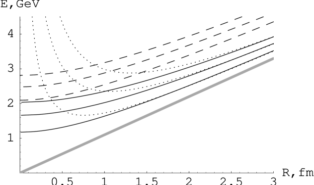
Figure 1: Adiabatic hybrid potentials in various regimes. Quasiclassical (solid line), potential (dashed), and flux-tube (dotted) curves for $n_{z}=n_{\rho}=0$ and $\Lambda=1,2,3$. The lowest curve is $\sigma R$. $\sigma=0.22$GeV².

The case of large $R$ can be treated directly in the full Hamiltonian (12), which in the small-oscillation limit takes the form

$$H=\frac{\mu}{2}+\frac{p^{2}_{z}}{2\mu}+\frac{p_{\perp}^{2}}{2(\mu+J_{1}+J_{2})}$$

$$+\sigma^{2}(\rho^{2}+(z+\frac{R}{2})^{2})\int^{1}_{0}\frac{d\beta_{1}}{2\nu_{1}}+\sigma^{2}(\rho^{2}+(z-\frac{R}{2})^{2})\int^{1}_{0}\frac{d\beta_{2}}{2\nu_{2}}$$

$$+\int^{1}_{0}{d\beta_{1}}\frac{\nu_{1}}{2}+\int^{1}_{0}{d\beta_{2}}\frac{\nu_{2}}{2},$$ (29)

displaying two different kinds of string excitations, along the $z$ axis and in the transverse direction. Indeed, for large $R$ one neglects the contribution of $\mu$ in the third term of (29) because the extremal values of $\nu_{1,2}$ are $\frac{\sigma R}{2}$. Then the oscillations in the longitudinal and transverse directions become uncoupled, and one has

$$E_{n}(R)=\sigma R+\frac{3}{2^{1/3}}\frac{\sigma^{1/3}(n_{z}+\frac{1}{2})^{2/3}}{R^{1/3}}+\frac{2\cdot 3^{1/2}}{R}(n_{\rho}+\Lambda+1).$$ (30)

The regime $\sim(\frac{\sigma}{R})^{1/3}$ is established at large $R$, but at the intermediate distances there are sizeble corrections from the string regime $\sim\Lambda/R$, as it is seen from Fig. 2.

Figure 2: Corrections to linear behaviour of potentials. QCD string (solid line), potential (dashed), and flux-tube (dotted) curves; $n_{z}=n_{\rho}=0$; $\sigma=0.22$GeV².

As we have not considered the spin of the gluon, we are not in the position yet to compare our predictions with lattice results [6]. Nevertheless, some preliminary conclusions can be drawn. For separations less than 2 fm the measured energies [6] lie much below Nambu-Goto curves (28). There is no universal Nambu-Goto behaviour even for $R$ as large as 4 fm. The QCD string model is able to describe both these features: at small separations the potential confinement regime dominates, while at large distances the situation is more complicated. Indeed, there is the contribution of the string-type gaps (27) which are due to transverse vibrations of the string, but the dominant subleading behaviour is defined by potential-type longitudinal motion. In particular, even for quasiclassically large values of $\Lambda$ there exists the contribution of oscillations in the longitudinal direction (second term in (30)).

Such peculiar behaviour displays the most pronounced difference between the given approach and other models of constituent glue. In contrast to phonon-type models, the QCD string vibrations are caused by point-like valence gluon, but, in contrast to potential models, the confining force follows from minimal area law, giving rise, at large distances, both to longitudinal vibrations with potential-type $\sim(\frac{\sigma}{r})^{1/3}$ dominant subleading behaviour and to the transverse vibrations with string-type $\sim\Lambda/R$ subleading behaviour, which could be responsible for the observed $\Lambda$ dependence. The full QCD string calculations with gluon spin involved will provide, if confirmed by the lattice data, the decisive evidence in favour of the QCD string model of valence glue.

We are grateful to Yu.A.Simonov for useful discussions. The support of INTAS-RFFI 97-0232, RFFI 00-02-17836 and 00-15-96786 grants is acknowledged.

References

• [1] A.I.Vainstein and L.B.Okun, Sov.J.Nucl.Phys. 23, 716 (1976).
• [2] D.Horn and J.Mandula, Phys.Rev. D17, 537 (1978).
• [3] E.S.Swanson and A.P.Szczepaniak, Phys.Rev. D59, 014035 (1999).
• [4] N.Isgur and J.Paton, Phys.Rev. D31, 2910 (1985).
• [5] A.Donnachie, P.R.Page, Phys.Rev. D59, 034016 (1999);
A.Donnachie and Yu.S.Kalashnikova, Phys.Rev. D60, 114011 (1999).
• [6] K.J.Juge, J.Kuti, and C.Morningstar, in Proc. of the Third Int. Conf. on Quark Confinement and the Hadron Spectrum, Jefferson Lab, 1998, hep-lat/9809015; in Proc. of LATTICE98, Boulder, USA, 1998, Nucl.Phys.Proc.Suppl. 73, 590 (1999).
• [7] Yu.A.Simonov, Lectures at the XVII International School of Physics, Lisbon, 1999, hep-ph/9911237.
• [8] A.Yu.Dubin, A.B.Kaidalov, and Yu.A.Simonov, Phys.Lett. B323, 41 (1994); Phys.At.Nucl. 56, 1745 (1993).
• [9] Yu.A.Simonov, in Proc. of Workshop on Physics and Detectors for DA$\Phi$NE, Frascati, 399 (1991); Yu.A.Simonov, in Proc. of HADRON’93 Conference, Como, 2629 (1993).
• [10] Yu.S.Kalashnikova and Yu.B.Yufryakov, Phys.Lett. B359, 175 (1995); Phys.At.Nucl. 60, 307 (1997).
• [11] A.B.Kaidalov and Yu.A.Simonov, Phys.Lett. B477, 163 (2000).
• [12] Yu.A.Simonov, Nucl.Phys. B592, 350 (2000).
• [13] Yu.A.Simonov, Phys.At.Nucl. 58, 107 (1995).
• [14] Yu.S.Kalashnikova and A.V.Nefediev, Phys.At.Nucl. 60, 1389 (1997).
• [15] V.L.Morgunov, A.V.Nefediev, and Yu.A.Simonov, Phys.Lett. B459, 653 (1999).
• [16] Yu.B.Yufryakov, Phys.At.Nucl. 59, 1636 (1996); preprint ITEP–56–95.