Abstract

We give an overview over recent calculations of baryonic correlator functions with finite mass quarks in view on their applicability for QCD sum rules. The QCD sum rule method is then demonstrated within the Heavy Quark Effective Theory.

1 Mesonic and baryonic correlators

Data sets which are produced to an huge amount especially by the so-called $B$ factories like Barbar, Belle, Cleo and Hera B allow for the discovery of excited states of hadrons containing the $b$ quark and other heavy quarks. In order to follow this development on the experimental side, theorists are asked to develop and use methods to analyze such excited states. There is one main obstacle on this way which consists of the scale differences that occur. While perturbative calculations including a heavy quark can effectively be done only in the high energy range, there is an extrapolation of these results down to the energy range needed where we expect excited states are to be located.

One of the most powerful methods which was developed long ago are the QCD sum rules. In this talk we will only concentrate on the QCD sum rule approach developed by Shifman, Vainshtein and Zakharov, called SVZ approach [1]. This approach makes special assumptions about the spectral density of the correlator function related to the hadron and uses the Borel transform for the extrapolation. There are a lot of calculations for the correlator function of hadrons, especially for those containing a heavy quark. The calculations were performed within perturbative QCD as well as HQET and the massless limit. In the first part of this talk I will concentrate on calculations using perturbative QCD. In all cases the baryons are a kind of “stepchild” of the theorists, so we work hard to fill this gap.

1.1 Baryonic correlators in QCD

The mesonic correlator function for two vector currents has already been calculated ten years ago by Generalis [2] even in the case of two different and non-vanishing masses. Our aim is therefore to extend these calculations to the baryonic case. A first step has already been done by a recent publication [3]. In this publication the spectral density is calculated for a three-quark current (two massless and one of finite mass) of the form

$$J_{B}=[u^{iT}Cd^{j}]\Psi^{k}\varepsilon_{ijk}.$$ (1)

The result presented in [3] is the one for the mass part $\Pi_{m}(-q^{2})$ of the correlator

$$\Pi(-q^{2})=q\kern-5.5pt/\Pi_{q}(-q^{2})+m\Pi_{m}(-q^{2}).$$ (2)

This part is independently interesting because it can directly be compared with the result obtained within HQET, as we will see later. The momentum part $\Pi_{q}(-q^{2})$ is still under construction, we expect a publication in the next few months. As mentioned before, we can easily reconstruct the correlator function

$$\Pi_{m}(-q^{2})=\int_{m^{2}}^{\infty}\frac{\rho_{m}(s)ds}{s-q^{2}}$$ (3)

if we know the spectral density. This is given by

$$\rho_{m}(s)=\frac{1}{128\pi^{4}}\rho(s),\qquad\rho=s^{2}\left\{\rho_{0}\left(1+\frac{\alpha_{s}}{\pi}\ln\left(\frac{\mu^{2}}{m^{2}}\right)\right)+\frac{\alpha_{s}}{\pi}\rho_{1}\right\}$$ (4)

where

$$\rho_{0}(s)=1+9z-9z^{3}-z^{3}+6z(1+z)\ln z$$ (5)

and

$$\rho_{1}(s)\ =\ 9+\frac{665}{9}z-\frac{665}{9}z^{2}-9z^{3}-\left(\frac{58}{9}+42z-42z^{2}-\frac{58}{9}z^{3}\right)\ln(1-z)\,+$$ (6)

$$+\left(2+\frac{154}{3}z-\frac{22}{3}z^{2}-\frac{58}{9}z^{3}\right)\ln z+4\left(\frac{1}{3}+3z-3z^{2}-\frac{1}{3}z^{3}\right)\ln(1-z)\ln z\,+$$

$$+12z\left(2+3z+\frac{1}{9}z^{2}\right)\left(\frac{1}{2}\ln^{2}z-\zeta(2)\right)+4\left(\frac{2}{3}+12z+3z^{2}-\frac{1}{3}z^{3}\right){\rm Li}_{2}(z)\,+$$

$$+24z(1+z)\left({\rm Li}_{3}(z)-\zeta(3)-\frac{1}{3}{\rm Li}_{2}(z)\ln z\right).$$

This result is obtained by using basic integrals of the kind

$$V(\alpha,\beta;q^{2}/m^{2})=\int\frac{d^{D}p}{(2\pi)^{D}}\frac{1}{(p^{2}+m^{2})^{\alpha}(q-p)^{2\beta}}$$ (7)

which are a generalization of the standard object $G(\alpha,\beta)$ of the massless calculation.

Figure 1: The ratio $\rho_{1}(s)/\rho_{0}(s)$ of the next-to-leading correction and the leading order term in dependence of the energy square $s$

1.2 Comparison with the limits

Here we only want to stress that we were able to compare this result with the two limits, i.e. the massless limit and the heavy quark or near-threshold limit. For the massless limit we obtain

$$m\rho(s)=m_{\overline{\rm MS}}(\mu)s^{2}\left\{1+\frac{\alpha_{s}}{\pi}\left(2\ln\left(\frac{\mu^{2}}{s}\right)+\frac{31}{3}\right)\right\}$$ (8)

where the relation between the pole (or invariant) mass parameter $m$ and the $\overline{\rm MS}$ mass $m_{\overline{\rm MS}}$ reads

$$m=m_{\overline{\rm MS}}\left\{1+\frac{\alpha_{s}}{\pi}\left(\ln\left(\frac{\mu^{2}}{m^{2}}\right)+\frac{4}{3}\right)\right\}.$$ (9)

With this explicit finite mass representation we can even obtain terms like $m^{2}\ln(\mu^{2}/m^{2})$ which are absent in the effective theory of massless quarks but result from perturbative contributions of heavy quark condensates $\langle\bar{\Psi}\Psi\rangle$. For the other limit, i.e. the near-threshold limit $E\rightarrow 0$ with $s=(m+E)^{2}$ we obtain

$$\rho^{\rm thr}(m,E)=\frac{16E^{5}}{5m}\left\{1+\frac{\alpha_{s}}{\pi}\ln\left(\frac{\mu^{2}}{m^{2}}\right)+\frac{\alpha_{s}}{\pi}\left(\frac{54}{5}+\frac{4\pi^{2}}{9}+4\ln\left(\frac{m}{2E}\right)\right)\right\}+O(E^{6}).$$ (10)

The invariant function $\rho_{m}$ suffices to determine the complete leading HQET behaviour since one has $q\kern-5.5pt/\rho_{q}+m\rho_{m}\rightarrow m(v\kern-5.0pt\raise 1.0pt\hbox{$\scriptstyle/$}\kern 1.0pt+1)\rho$ for the leading term. In this region the appropriate device to compute the limit of the correlator is HQET (see e.g. [4, 5]). Writing

$$m\rho^{\rm thr}(m,E)=C(m/\mu,\alpha_{s})^{2}\rho^{\rm HQET}(E,\mu)$$ (11)

we obtain the known result for $\rho^{\rm HQET}(E,\mu)$ [6] with matching coefficient $C(m/\mu,\alpha_{s})$ [7]. In this case the matching procedure allows one to restore the near-threshold limit of the full correlator starting from the simpler effective theory near threshold [8] (see also [9]). Note that the higher order corrections in $E/m$ to Eq. (10) can be easily obtained from the explicit result given in Eq. (6). Indeed, the next-to-leading order correction in low energy expansion reads

$$\Delta\rho^{\rm thr}(m,E)=-\frac{88E^{6}}{5m^{2}}\left\{1+\frac{\alpha_{s}}{\pi}\left(\ln\left(\frac{\mu^{2}}{m^{2}}\right)+\frac{376}{33}+\frac{4\pi^{2}}{9}+\frac{140}{33}\ln\left(\frac{m}{2E}\right)\right)\right\}.$$ (12)

It is a much more difficult task to obtain this result starting from HQET. In Fig. 1 we compare components of the baryonic spectral function in leading and next-to-leading order. Shown is the ratio $\rho_{1}(s)/\rho_{0}(s)$ where we put $\mu=m$ for simplicity. One can see that a simple interpolation between the two limits can give a rather good approximation for the next-to-leading order correction in the complete region of $s$.

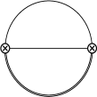
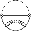
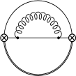
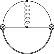
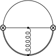
Figure 2: The calculated two-loop and three-loop topologies

1.3 A specific feature of the calculation

The two-loop and three-loop Feynman diagrams which had to be calculated for the determination of the spectral function are shown in Fig. 2. For our calculation we extensively used the fact that the diagrams can be composed by glueing together subdiagrams (see also Ref. [10]). The so-called scalar spectacle diagram in Fig. 3 is calculated as the convolution of two heavy-light spectral densities,

$$\rho(s)=\int\lambda(s,s_{1},s_{2})\rho_{1}(s_{1})\rho_{2}(s_{2})ds_{1}ds_{2}$$ (13)

where the convolution function is given by the remaining line.

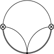
Figure 3: The scalar spectacle diagram

2 QCD sum rules for the HQET

The QCD sum rules for the correlator calculated above have not yet been constructed. Instead we will present the principles of the SVZ approach to QCD sum rules as applied to leading order HQET with results for heavy baryons taken from previous publications [6, 11].

2.1 Construction of QCD sum rules

The QCD sum rules can be constructed by taking care of two possible expressions for the two-point correlator which in this case reduces to a scalar correlator function $P(\omega)$,

$$\Pi(\omega=p\cdot v)=i\int e^{ip\cdot x}\langle T\{J(x),\bar{J}(0)\}\rangle d^{4}x=\Gamma^{\prime}\frac{1+v\kern-5.0pt\raise 1.0pt\hbox{$\scriptstyle/$}\kern 1.0pt}{2}\bar{\Gamma}^{\prime}\frac{1}{2}{\rm Tr}(\Gamma\bar{\Gamma})2{\rm\,Tr}(\tau\tau^{\dagger})P(\omega).$$ (14)

On the one hand side, the function $P(\omega)$ satisfies the dispersion relation

$$P(\omega)=\int_{0}^{\infty}\frac{\rho(\omega^{\prime})d\omega^{\prime}}{\omega^{\prime}-\omega-i0}+\mbox{subtraction},$$ (15)

where $\rho(\omega)$ is the spectral density in HQET. On the phenomenological side the two-point correlator is represented by the spectral representation

$$P(\omega)=\frac{\frac{1}{2}|F_{B}|^{2}}{\bar{\Lambda}-\omega-i0}+\sum_{X\neq B}\frac{\frac{1}{2}|F_{X}|^{2}}{\omega_{X}-\omega-i0}+\mbox{subtr.}$$ (16)

where $\bar{\Lambda}=m_{B}-m_{Q}$ is the ground state energy of the baryon and $F_{B}$ the residue. The main assumption of the SVZ approach is that the remaining sum can be approximated by the integral of the spectral density given by the dispersion relation and starting from some threshold energy $E_{C}$. The combination of the phenomenological and the theoretical identity for the correlator function then leads to

$$\frac{\frac{1}{2}|F_{B}|^{2}}{\bar{\Lambda}-\omega-i0}=\int_{0}^{E_{C}}\frac{\rho(\omega^{\prime})d\omega^{\prime}}{\omega^{\prime}-\omega-i0}+\mbox{subtr.}$$ (17)

2.2 The Borel transformation

This formula is not useful since the spectral density as calculated in the Euklidean domain is reliable only for negative values of $\omega$, while the integral is to be calculated mainly at $\omega=\bar{\Lambda}$. This region of integration can be reached by an extrapolation using higher and higher derivatives when $\omega$ goes to $-\infty$. This extrapolation is expressed by the Borel transformation (cf. e.g. Ref. [5])

$$\hat{B}_{T}^{(\omega)}(f(\omega))=\lim_{-\omega,n\rightarrow\infty}\frac{(-\omega)^{n+1}}{n!}\frac{d^{n}}{d\omega^{n}}f(\omega),\qquad T=\frac{-\omega}{n}\quad\mbox{fixed}.$$ (18)

The Borel transformation is by construction a derivative and therefore also cancels the (constant) subtraction terms. The Borel parameter $T$ is an unphysical quantity in units of an energy, and the obtained values should be mostly independent on this parameter. This will be the main criterion in analyzing the sum rules. The Borel transformation leads to the final form of the QCD sum rule,

$$\frac{1}{2}|F_{B}|^{2}e^{-\bar{\Lambda}/T}=K(E_{C},T),\qquad K(E_{C},T)=\int_{0}^{E_{C}}\rho(\omega)e^{-\omega/T}d\omega+\sum_{i}\frac{A_{i}}{T^{i}}.$$ (19)

At the end we can take the derivative with respect to the inverse Borel parameter and obtain a second sum rule,

$$\bar{\Lambda}=-\frac{1}{2}\frac{\partial}{\partial(T^{-1})}\ln K(E_{C},T).$$ (20)

(a)(b)(c)(d)

Figure 4: Sum rule analysis for the heavy baryon $\Lambda_{Q}$. Shown are five curves for five different values of the threshold energy $E_{C}$ spaced by $100{\rm\,MeV}$ around the central value $E_{C}=E_{C}^{\rm best}$. $E_{C}$ grows from bottom to top. The figure parts are in detail (a) the lowest order sum rule results and (b) the $O(\alpha_{s})$ sum rule results for the bound state energy $\bar{\Lambda}$, (c) the lowest order sum rule results and (d) the $O(\alpha_{s})$ sum rule results for the absolute value of the residue $F_{\Lambda}$.

2.3 QCD sum rule analysis

The procedure of the sum rule analysis is as follows: First we calculate the theoretical expression for $K(E_{C},T)$ by calculating the spectral density within perturbation theory. This has been done for the next-to-leading order of the $d=0$ term as well as the $d=3$ term in the Operator Product Expansion. For brevity I will only mention the results of the analysis for the $d=0$ radiative corrections. For the analysis we have to select a “sum rule window”, i.e. a range for the Borel parameter $T$ in which the sum rule analysis is performed. The boundaries of this window is given by heuristic arguments. If the Borel parameter becomes too small, the nonperturbative contributions which are badly known blow up. If on the other hand the Borel parameter becomes too large, the fact that the Borel parameter appears as “temperature” in the sum rule causes the problem that higher and higher excitations contribute to the ground state. The region of reliability and so the sum rule window is therefore roughly given by $\Lambda_{\rm QCD}<T<2\bar{\Lambda}$.

Now we use the second sum rule (20) to determine the ground state energy parameter $\bar{\Lambda}$. This is done by varying the continuum threshold parameter $E_{C}$ in order to obtain a rather stable value for the quantities with respect to the unphysical parameter $T$ within the sum rule window. The value obtained for the ground state energy can then be used in the first sum rule (19) to determine the absolute value $|F_{B}|$ of the residue. More detailed considerations are found in Ref. [6]. Our results read

$$E_{C}(\Lambda_{Q}) = 1.2\pm 0.1{\rm\,GeV},$$

$$\bar{\Lambda}(\Lambda_{Q}) = 0.77\pm 0.05{\rm\,GeV},$$ (21)

$$|F(\Lambda_{Q})| = 0.022\pm 0.001{\rm\,GeV}^{3}$$

while the $O(\alpha_{s})$ results are given by

$$E_{C}(\Lambda_{Q}) = 1.1\pm 0.1{\rm\,GeV},$$

$$\bar{\Lambda}(\Lambda_{Q}) = 0.77\pm 0.05{\rm\,GeV},$$ (22)

$$|F(\Lambda_{Q})| = 0.027\pm 0.001{\rm\,GeV}^{3}$$

where the errors are estimated by looking at the stability with respect to different values for $E_{C}$. Taking the experimental results for the masses of the baryons, namely $m(\Lambda_{c})=2284.9\pm 0.6{\rm\,MeV}$ and $m(\Lambda_{b})=5642\pm 50{\rm\,MeV}$ [12], our central value $\bar{\Lambda}(\Lambda_{Q})$ for the bound state energy suggests pole masses of $m_{c}=1520\pm 100{\rm\,MeV}$ and $m_{b}=4880\pm 100{\rm\,MeV}$.

3 Conclusion and Outlook

The QCD sum rule analysis for heavy baryons requires the calculation of the spectral density related to the correlator function of baryonic currents. If this spectral density is calculated, the sum rule analysis can be used as powerful tool to extract phenomenological non-perturbative quantities like bound state energies and form factors. I have presented the sum rule analysis for an example within HQET. In order to perform a sum rule analysis for baryons containing finite mass quarks the following steps are still missing and will be done in the near future:

• The calculation of the momentum part of the spectral density (nearly finished)

• The matching procedure for the spectral density

• The calculation of spectral densities for baryons with different quantum numbers

Moreover it is planned to develop light-cone sum rules for the three-point function of heavy baryons in order to determine the Isgur-Wise function.

Acknowledgments

I want to thank my collaborators J.G. Körner, A.A. Pivovarov and O.I. Yakovlev for the continuing and fruitful collaboration. I would like to thank the organizers of this conference for their hospitality. This work is supported by a grant given by the DFG.

References

- [1] M.A. Shifman, A.I. Vainshtein and V.I. Zakharov, Nucl. Phys. B147 (1979) 385; B147 (1979) 448
- [2] S.C. Generalis, J. Phys. G16 (1990) 785
- [3] S. Groote, J.G. Körner and A.A. Pivovarov, Phys. Rev. D61 (2000) 071501
- [4] H. Georgi, Nucl. Phys. B363 (1991) 301
- [5] M. Neubert, Phys. Rep. 245 (1994) 259
- [6] S. Groote, J.G. Körner and O.I. Yakovlev, Phys. Rev. D55 (1997) 3016
- [7] A.G. Grozin and O.I. Yakovlev, Phys. Lett. 285 B (1992) 254
- [8] E. Eichten and B. Hill, Phys. Lett. 234 B (1990) 511
- [9] S. Groote and A.A. Pivovarov, “Threshold expansion of Feynman diagrams within a configuration space technique”, Report No. MZ-TH/00-07, hep-ph/0003115, to be published in Nucl. Phys. B
- [10] S. Groote, J.G. Körner and A.A. Pivovarov, Nucl. Phys. B542 (1999) 515; Eur. Phys. J. C11 (1999) 279; Phys. Lett. 443 B (1998) 269
- [11] S. Groote, J.G. Körner and O.I. Yakovlev, Phys. Rev. D56 (1997) 3943
- [12] Particle Data Group, “Review of Particle Properties”, Eur. Phys. J. C3 (1998) 1