On the Inclusive Determination of $|V_{ub}|$ from the Lepton Invariant Mass Spectrum

Abstract:

Bauer, Ligeti and Luke have recently proposed a new method for measuring $|V_{ub}|$ in inclusive semileptonic $B$ decays, using a cut $\sqrt{q^{2}}>M_{B}-M_{D}$ on the lepton invariant mass to discriminate against $b\to c$ transitions. We investigate the structure of the heavy-quark expansion for this case and show that to all orders the magnitude of the leading perturbative and nonperturbative corrections is controlled by a hadronic scale $\mu_{c}\ \hbox to0.0pt{\raise 3.0pt\hbox{$<$}\hss}{\lower 3.0pt\hbox{$\sim$}}\ m_{c}$ depending on the minimal value of $q^{2}$. These corrections can be analyzed using a modified version of the heavy-quark expansion (“hybrid expansion”). We find that the theoretical uncertainty in the extraction of $|V_{ub}|$ is a factor 2.5 larger than previously estimated, which allows for a determination with 10% accuracy.

(Submitted to Journal of High Energy Physics)

1 Introduction

A precise knowledge of the magnitude of the Cabibbo–Kobayashi–Maskawa (CKM) matrix element $V_{ub}$ is of great importance to the study of CP violation at the $B$ factories. Whereas the main target of CP-asymmetry measurements is to fix the angles of the unitarity triangle, the length of the sides of this triangle are determined by the smallest CKM elements, $|V_{ub}|$ and $|V_{td}|$. The measurement of $|V_{ub}|$, which neither involves CP violation nor rare loop processes, appears to be the simplest step in the overall determination of the unitarity triangle. Yet, at present this measurement is limited by uncomfortably large theoretical uncertainties.

$|V_{ub}|$ can be determined most directly from semileptonic $B$ decays into charmless final states. The theoretical interpretation of exclusive decays such as $B\to\pi\,l\,\nu$ or $B\to\rho\,l\,\nu$ is limited by the necessity to predict the $B\to\pi$ or $B\to\rho$ transition form factors, which parameterize the complicated hadronic interactions relevant to these decays. The inclusive decays $B\to X\,l\,\nu$ admit a cleaner theoretical analysis based on a heavy-quark expansion [1, 2, 3]. However, an obstacle is that experimentally it is necessary to impose restrictive cuts to suppress the background from $B\to X_{c}\,l\,\nu$ decays (i.e., decays into final states with charm). Accounting for such cuts theoretically is difficult and usually introduces significant uncertainties.

The first determination of $|V_{ub}|$ from inclusive decays was based on a measurement of the charged-lepton energy spectrum close to the endpoint region, which is kinematically forbidden for decays with a charm hadron in the final state. This restriction eliminates about 90% of the $B\to X_{u}\,l\,\nu$ signal, and it is difficult to calculate reliably the small fraction of the remaining events. The reason is that in this portion of phase space the conventional heavy-quark expansion breaks down and must be replaced by a twist expansion, in which an infinite tower of local operators is resummed into a shape function describing the light-cone momentum distribution of the $b$ quark inside a $B$ meson [4, 5, 6]. A promising strategy is to infer the fraction of semileptonic decays in the endpoint region from a study of the photon spectrum in $B\to X_{s}\,\gamma$ decays, since the leading nonperturbative effects in the two decays are described by the same shape function [6, 7, 8, 9]. Recently, it has been emphasized that a cut $M_{X}<M_{D}$ on the hadronic invariant mass would provide for a better discrimination between $B\to X_{u}\,l\,\nu$ and $B\to X_{c}\,l\,\nu$ decays [10, 11, 12]. Such a cut eliminates the charm background, while affecting only about 20% of the signal events. Despite of this advantage, however, it is difficult to calculate precisely what this fraction is [13].

Bauer, Ligeti and Luke (BLL) have pointed out that the situation may be better if a discrimination based on a cut on the lepton invariant mass $\sqrt{q^{2}}$ is employed [14]. Requiring $q^{2}>(M_{B}-M_{D})^{2}$ eliminates the charm background, while containing about 20% of the signal events. This fraction is much less than in the case of a cut on hadronic invariant mass, but the inclusive rate with a lepton invariant mass cut offers the advantage of being calculable using a conventional heavy-quark expansion, without a need to resum an infinite series of nonperturbative corrections. BLL find that the fraction of $B\to X_{u}\,l\,\nu$ events with $q^{2}>q_{0}^{2}$, where $q_{0}^{2}\geq(M_{B}-M_{D})^{2}$ is required to eliminate the charm background, is given by

$$F(q_{0}^{2})=(1+\hat{q}_{0}^{2})(1-\hat{q}_{0}^{2})^{3}+\tilde{X}(\hat{q}_{0}^{2})\,\frac{\alpha_{s}(m_{b})}{\pi}-\left(\hat{q}_{0}^{2}-2\hat{q}_{0}^{6}+\hat{q}_{0}^{8}\right)\frac{12\lambda_{2}}{m_{b}^{2}}+\dots\,,$$ (1)

where $\hat{q}_{0}^{2}=q_{0}^{2}/m_{b}^{2}$, and the dots represent corrections of higher order in the expansion in powers of $\alpha_{s}(m_{b})$ and $\Lambda/m_{b}$ (with $\Lambda$ a characteristic hadronic scale). The function $\tilde{X}(\hat{q}_{0}^{2})$ can be obtained from results presented in [15]. The nonperturbative parameter $\lambda_{2}=\frac{1}{4}(M_{B^{*}}^{2}-M_{B}^{2})\simeq 0.12$ GeV² was introduced in [16]. As it stands, eq. (1) seems to provide a solid theoretical basis for a systematic analysis of the partial decay rate in an expansion in logarithms and powers of $\Lambda/m_{b}$. (This leaves aside the fact that the lepton invariant mass cut eliminates about 80% of all $B\to X_{u}\,l\,\nu$ events, and therefore one may worry that violations of quark–hadron duality may be larger than for the total inclusive semileptonic rate.)

The purpose of this work is to analyze the structure of the result (1) in more detail. We show that the relevant mass scale $\mu_{c}$ controlling the size of corrections in the heavy-quark expansion is less than or of order the charm-quark mass, rather than the heavier $b$-quark mass. This is so because the largest values of the hadronic invariant mass and energy accessible are of order the charm mass or less. Although the ratio $m_{c}/m_{b}$ is usually taken as a constant when discussing the heavy-quark limit, it is well known that the convergence of heavy-quark expansions at the charm scale can be poor. This makes our observation relevant. We suggest that an appropriate framework in which to investigate the leading corrections to the heavy-quark limit in the present case is a modified version of the heavy-quark expansion to which we refer as “hybrid expansion”. The idea is that in the kinematic region where $M_{B}\gg E_{X}\sim M_{X}\gg\Lambda$ one can perform a two-step expansion in the ratios $E_{X}/M_{B}$ and $\Lambda/E_{X}$. A similar strategy has been used in applications of the heavy-quark effective theory (HQET) to resum the so-called “hybrid logarithms” $\alpha_{s}\ln(m_{c}/m_{b})$ [17] arising in current-induced $b\to c$ transitions using renormalization-group (RG) equations [18, 19]. In the context of inclusive decays, an approach similar in spirit to our proposal was suggested first by Mannel [20]. We use the hybrid expansion to obtain a RG-improved expression for the perturbative corrections to the quantity $F(q_{0}^{2})$ at next-to-leading order (NLO), as well as to estimate the size of higher-order power corrections omitted in (1).

2 Structure of the hadronic tensor

The strong-interaction dynamics relevant to inclusive $B$ decays is encoded in a hadronic tensor defined as the forward matrix element of the time-ordered product of two weak currents between $B$-meson states. Although the variable of prime interest to our discussion is the lepton invariant mass, the physics of the hadronic tensor is most naturally described in terms of the hadronic invariant mass and energy, $M_{X}$ and $E_{X}$. These variables are related by $q^{2}=M_{B}^{2}-2M_{B}E_{X}+M_{X}^{2}$, and thus the restriction $q^{2}>q_{0}^{2}$ implies

$$M_{X}\leq E_{X}\leq\frac{M_{B}^{2}+M_{X}^{2}-q_{0}^{2}}{2M_{B}}\,,\qquad M_{\pi}^{2}\leq M_{X}^{2}\leq(M_{B}-\sqrt{q_{0}^{2}})^{2}\,.$$ (2)

With the optimal choice $q_{0}^{2}=(M_{B}-M_{D})^{2}$ this gives $M_{\pi}\leq M_{X}\leq M_{D}$ and $M_{X}\leq E_{X}\leq M_{D}-\frac{1}{2}(M_{D}^{2}-M_{X}^{2})/M_{B}$. Both variables vary between $M_{\pi}$ and $M_{D}$. If the cutoff $q_{0}^{2}$ is chosen higher, as may be required for experimental reasons, their maximal values become less than $M_{D}$.

The corresponding variables entering a partonic description of inclusive decay rates are the parton invariant mass and energy, $\sqrt{p^{2}}$ and $v\cdot p$, where $p$ is related to the lepton momentum $q$ by $p=m_{b}v-q$, and $v$ is the velocity of the $B$ meson. The phase space for the dimensionless variables $\hat{p}^{2}=p^{2}/m_{b}^{2}$ and $z=2v\cdot p/m_{b}$ is

$$2\sqrt{\hat{p}^{2}}\leq z\leq 1-\hat{q}_{0}^{2}+\hat{p}^{2}\,,\qquad 0\leq\hat{p}^{2}\leq(1-\sqrt{\hat{q}_{0}^{2}})^{2}\,.$$ (3)

For the purpose of our discussion here $m_{b}$ is the pole mass of the $b$ quark. Alternative mass definitions will be discussed in more detail later. The optimal value of $\hat{q}_{0}^{2}$ is $\hat{q}_{0}^{2}=(M_{B}-M_{D})^{2}/m_{b}^{2}\simeq(1-\frac{m_{c}}{m_{b}})^{2}$. In this case the largest values of the parton variables are $z_{\rm max}=2\,\frac{m_{c}}{m_{b}}$ and $\hat{p}^{2}_{\rm max}=(\frac{m_{c}}{m_{b}})^{2}$. Without a restriction on $q^{2}$, the phase space for these variables would be such that $z_{\rm max}=2$ and $\hat{p}^{2}_{\rm max}=1$. In other words, the lepton invariant mass cut restricts both variables to a region where they are parametrically suppressed, such that $v\cdot p$ and $\sqrt{p^{2}}$ are at most of order $m_{c}$. Besides $m_{b}$, the charm-quark mass is then a relevant scale that determines the magnitude of strong-interaction effects in the heavy-quark expansion.

To make the parametric suppression noted above more explicit, we introduce a characteristic scale $\mu_{c}$ and an associated small expansion parameter $\epsilon$ by

$$\mu_{c}=\frac{m_{b}^{2}-q_{0}^{2}}{2m_{b}}=O(m_{c})\,,\qquad\epsilon=\frac{1-\hat{q}_{0}^{2}}{2}=\frac{\mu_{c}}{m_{b}}\,,$$ (4)

and rewrite the fraction $F(q_{0}^{2})$ of $B\to X_{u}\,l\,\nu$ events with $q^{2}>q_{0}^{2}$ as

$$F(\epsilon)=16\epsilon^{3}(1-\epsilon)\left[C_{0}(\epsilon)-\frac{3}{2}\,C_{2}(\epsilon)\,\frac{\lambda_{2}}{\mu_{c}^{2}}+O[(\Lambda/\mu_{c})^{3}]\right]\,,$$ (5)

where $C_{n}(\epsilon)=1+O(\epsilon,\alpha_{s})$ are short-distance coefficients. From (1) we find

$$C_{0}(\epsilon) = 1+\frac{\alpha_{s}}{3\pi}\left[\left(-6\ln 2\epsilon-\frac{3}{2}-\frac{2\pi^{2}}{3}\right)+\epsilon\left(-8\ln 2\epsilon+\frac{73}{6}\right)+O(\epsilon^{2})\right]+O(\alpha_{s}^{2})\,,$$

$$C_{2}(\epsilon) = \frac{1-8\epsilon^{2}+8\epsilon^{3}}{1-\epsilon}+O(\alpha_{s})\,.$$ (6)

The definition of $\epsilon$ and $\mu_{c}$, as well as the explicit form of the coefficients $C_{n}(\epsilon)$, depend on the definition of the heavy-quark mass. The above result for $C_{0}(\epsilon)$ refers to the pole mass. Later we will introduce a more suitable mass definition and give an exact NLO expression for $C_{0}(\epsilon)$ including the higher-order terms in $\epsilon$.

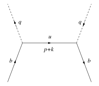
Figure 1: Tree-level contribution to the hadronic tensor. Dashed lines represent the weak currents.

It is apparent from (5) that the leading power correction proportional to $\lambda_{2}$ is of order $(\Lambda/\mu_{c})^{2}$. It is not difficult to see that, in the presence of a lepton invariant mass cut, also in higher orders the power corrections scale like $(\Lambda/\mu_{c})^{n}$. For simplicity of the argument we work to leading order in $\alpha_{s}$, where only the tree diagram shown in Figure 1 contributes to the hadronic tensor. In momentum space, the $u$-quark propagator gives a contribution

$$\frac{(p+k)^{\mu}}{p^{2}+2p\cdot k+k^{2}}\,,$$ (7)

where $k=O(\Lambda)$ is the residual momentum of the heavy quark inside the $B$ meson [21]. Roughly speaking, the heavy-quark expansion is obtained by replacing the residual momentum with a covariant derivative, $k^{\mu}\to iD^{\mu}$, thereby introducing the soft interactions of the $u$-quark jet with the background field of the light degrees of freedom in the $B$ meson. Let us discuss how the three terms in the denominator of the propagator scale in the different kinematic regions relevant to the determination of $|V_{ub}|$. Whereas the $k^{2}\sim\Lambda^{2}$ term is always suppressed, the relative magnitude of the two other terms depends on the kinematic region considered. For the regions of the large charged-lepton energy or low hadronic invariant mass, the terms $p^{2}\sim\max[\Lambda\,m_{b},m_{c}^{2}]$ and $p\cdot k\sim\Lambda\,m_{b}$ are of the same magnitude, and it is thus necessary to resum terms of the form $(p\cdot k/p^{2})^{n}$ to all orders in the heavy-quark expansion. This leads to a twist expansion, where these terms are absorbed into a nonperturbative shape function [4, 5, 6]. In contrast, for large lepton invariant mass, $p\cdot k\sim\Lambda\,m_{c}$ is parametrically suppressed with respect to $p^{2}\sim m_{c}^{2}$ by a power of $\Lambda/m_{c}$.

These general observations can also be derived from the explicit expression for the differential decay rate expressed in terms of the variables $z$ and $\hat{p}^{2}$, normalized to the total decay rate. At NLO in the heavy-quark expansion we find

$$\frac{1}{\Gamma}\,\frac{\mbox{d}^{2}\Gamma}{\mbox{d}z\,\mbox{d}\hat{p}^{2}} = 2z^{2}(3-2z)\,\delta(\hat{p}^{2})+\frac{\alpha_{s}}{3\pi}\,E(z,\hat{p}^{2})$$ (8)

$$\mbox{}-\delta(\hat{p}^{2})\left[\frac{z}{3}\,(36-27z-16z^{2})\,\frac{\lambda_{1}}{m_{b}^{2}}+(12+12z-63z^{2}+8z^{3})\,\frac{\lambda_{2}}{m_{b}^{2}}\right]$$

$$\mbox{}-\delta^{\prime}(\hat{p}^{2})\left[\frac{z^{2}}{3}\,(18+3z-14z^{2})\,\frac{\lambda_{1}}{m_{b}^{2}}+z^{2}(6+3z-10z^{2})\,\frac{\lambda_{2}}{m_{b}^{2}}\right]$$

$$\mbox{}-\delta^{\prime\prime}(\hat{p}^{2})\,\frac{z^{4}}{3}\,(3-2z)\,\frac{\lambda_{1}}{m_{b}^{2}}+\dots\,,$$

where $\lambda_{1}$ is a nonperturbative parameter related to the average kinetic energy of the $b$ quark inside the $B$ meson [16], and the function $E(z,\hat{p}^{2})$ gives the perturbative correction calculated in [13], which also includes the correction to the total decay rate appearing in the denominator on the left-hand side. The power corrections in (8) have been derived using the results of [3, 22]. In the kinematic region where $z=O(\epsilon)$ and $\hat{p}^{2}=O(\epsilon^{2})$, it is instructive to change variables from $(z,\hat{p}^{2})$ to $(z,\xi)$, where $\xi=4\hat{p}^{2}/z^{2}=p^{2}/(v\cdot p)^{2}\in[0,1]$ is related to the parton velocity in the $B$ rest frame. The kinematic range for these variables is

$$0\leq\xi\leq 1\,,\qquad 0\leq z\leq\frac{2}{\xi}\,(1-\sqrt{1-2\epsilon\xi})=2\epsilon+\epsilon^{2}\xi+O(\epsilon^{3})\,.$$ (9)

The variable $\xi$ is of order unity irrespective of the lepton invariant mass cut. Thus, after the transformation the only parametrically small quantity is $z=O(\epsilon)$. In terms of the new variables, the double-differential decay rate turns into an expansion in powers of $\Lambda/(zm_{b})$, and the perturbative corrections contain single logarithms of $z$. Integrating the double-differential rate over $z$, and keeping only terms of leading order in $\epsilon$, we obtain

$$\frac{1}{\Gamma}\,\frac{\mbox{d}\Gamma}{\mbox{d}\xi} = 16\epsilon^{3}\Bigg{\{}\delta(\xi)\left[1-\frac{\alpha_{s}}{3\pi}\left(6\ln\frac{\mu_{c}}{m_{b}}+8\ln 2(\ln 2-1)+\frac{31}{2}\right)\right]-$$ (10)

$$\mbox{}-\frac{\alpha_{s}}{3\pi}\left[\frac{4\ln\xi}{\xi}+\frac{1}{\xi}\left(7\sqrt{1-\xi}-8\ln(1+\sqrt{1-\xi})\right)\right]_{+}$$

$$\mbox{}-\frac{3\lambda_{2}}{2\mu_{c}^{2}}\,\delta(\xi)-\frac{3(\lambda_{1}+\lambda_{2})}{\mu_{c}^{2}}\,\delta^{\prime}(\xi)-\frac{2\lambda_{1}}{\mu_{c}^{2}}\,\delta^{\prime\prime}(\xi)+\dots\Bigg{\}}+O(\epsilon^{4})\,.$$

The integral of this expression over $\xi$ reproduces the leading terms in $\epsilon$ in (5). The result for the power corrections shows that indeed $\mu_{c}=O(m_{c})$ is the characteristic scale of the hybrid expansion. Perturbative logarithms of $\mu_{c}/m_{b}$ appear because the intrinsic scale of the hadronic tensor is smaller than the mass of the external $b$ quarks, suggesting that the appropriate scale to evaluate the running coupling $\alpha_{s}$ is significantly less than $m_{b}$. This is in accordance with the observation [23] that the physical scale derived using the Brodsky–Lepage–Mackenzie (BLM) scale-setting prescription [24] strongly decreases with increasing $q^{2}$. We will come back to the question of scale setting in the next section.

Figure 2: Contour representation of $F(q_{0}^{2})$ in the complex $\hat{p}^{2}$ plane.

For later purposes, it will be useful to have yet another way of reproducing the result (5). To this end, we represent the fraction $F(q_{0}^{2})$ as a contour integral in the complex $\hat{p}^{2}$ plane. Such a representation exists because the hadronic tensor is an analytic function in the complex plane apart from discontinuities located on the positive real $\hat{p}^{2}$ axis, as illustrated in Figure 2. We write

$$F(q_{0}^{2})=\frac{i}{2\pi}\oint\limits_{|\hat{p}^{2}|=\hat{p}^{2}_{\rm max}}\!\!\!\mbox{d}\hat{p}^{2}\,T(\hat{p}^{2},\hat{q}_{0}^{2})\,,$$ (11)

where $\hat{p}_{\rm max}^{2}=(1-\sqrt{\hat{q}_{0}^{2}})^{2}$, and the correlator $T(\hat{p}^{2},\hat{q}_{0}^{2})$ can be obtained using dispersion relations [13]. Eliminating $\hat{q}_{0}^{2}$ in favor of $\epsilon$, and parameterizing $\hat{p}^{2}=\hat{p}^{2}_{\rm max}\,e^{i\varphi}$ on the contour of integration, the result can be written in the form

$$F(\epsilon)=16\epsilon^{3}(1-\epsilon)\int\limits_{0}^{2\pi}\frac{\mbox{d}\varphi}{2\pi}\,t(e^{i\varphi},\epsilon)\,,$$ (12)

where the function $t(e^{i\varphi},\epsilon)$ contains the corrections to the heavy-quark limit. We obtain

$$t(e^{i\varphi},\epsilon) = C_{0}(\epsilon)+\frac{\alpha_{s}}{3\pi}\,Y(e^{i\varphi},\epsilon)-\frac{3}{2}\,C_{2}(\epsilon)\,\frac{\lambda_{2}}{\mu_{c}^{2}}+\left[D_{1}(\epsilon)\,\frac{\lambda_{1}}{\mu_{c}^{2}}+D_{2}(\epsilon)\,\frac{\lambda_{2}}{\mu_{c}^{2}}\right]e^{-i\varphi}$$ (13)

$$\mbox{}-\frac{4}{5}\,E_{1}(\epsilon)\,\frac{\lambda_{1}}{\mu_{c}^{2}}\,e^{-2i\varphi}+O[(\Lambda/\mu_{c})^{3}]\,.$$

The function $Y(e^{i\varphi},\epsilon)$ with

$$Y(x,\epsilon)=\frac{10}{3}\,x-\frac{184}{9}+\left(\frac{29}{3}-\frac{5}{3}\,x\right)u\ln\frac{u+1}{u-1}-2\ln^{2}\frac{u+1}{u-1}+O(\epsilon)$$ (14)

and $u=\sqrt{1-x}$ is defined such that its contour integral vanishes. The coefficients $D_{i}(\epsilon)$ and $E_{1}(\epsilon)$ are equal to 1 in the limit $\epsilon\to 0$. Their explicit expressions are

$$D_{1}(\epsilon) = \frac{\epsilon^{2}}{(1-\epsilon)(1-\sqrt{1-2\epsilon})^{2}}\left(1-\frac{7}{4}\,\epsilon+\frac{4}{5}\,\epsilon^{2}\right)+O(\alpha_{s})\,,$$

$$D_{2}(\epsilon) = \frac{\epsilon^{2}}{(1-\epsilon)(1-\sqrt{1-2\epsilon})^{2}}\left(1+\frac{3}{4}\,\epsilon-4\epsilon^{2}\right)+O(\alpha_{s})\,,$$

$$E_{1}(\epsilon) = \frac{\epsilon^{4}}{(1-\epsilon)(1-\sqrt{1-2\epsilon})^{4}}\left(1-\frac{10}{9}\,\epsilon\right)+O(\alpha_{s})\,.$$ (15)

Equations (10) and (13) allow us to study the behavior of the leading corrections in the heavy-quark expansion in more detail. In particular, we will utilize them to estimate unknown, higher-order power corrections. We will, however, first investigate the perturbative corrections in more detail, using the hybrid expansion as a tool to perform a systematic RG improvement of the one-loop expressions in (1) and (2).

3 RG improvement and definition of the heavy-quark mass

Based on the observation that the event fraction $F(q_{0}^{2})$ in (1) receives very small corrections of order $\beta_{0}\alpha_{s}^{2}$, where $\beta_{0}$ is the first coefficient of the $\beta$-function, BLL have argued that the perturbative uncertainty in their prediction is negligible [14]. The purpose of this section is to critically reanalyze the perturbative uncertainty in the calculation of this quantity. We first note that in the present case it is misleading to associate the size of $\beta_{0}\alpha_{s}^{2}$ corrections with a physical BLM scale in the process. The total semileptonic rate and the lepton invariant mass spectrum receive very large corrections of order $\beta_{0}\alpha_{s}^{2}$, corresponding to very low BLM scales [23]. The fraction $F(\epsilon)$ is defined as the ratio of the partially integrated lepton spectrum and the total rate. If both of these quantities have low physical scales, the same must be true for their ratio. In our opinion the small $\beta_{0}\alpha_{s}^{2}$ correction observed in [14] is thus due to an accidental cancellation and does not bare any physical significance.

Here we follow a different strategy to estimate the potential importance of higher-order effects. We have argued that a useful framework in which to analyze the fraction $F(\epsilon)$ is provided by a hybrid expansion, in which the physics associated with the three mass scales $m_{b}\gg\mu_{c}\gg\Lambda$ is disentangled. Since the intermediate scale $\mu_{c}$ is only about 1 GeV or less, and since the running of the strong coupling in the region between $m_{b}$ and 1 GeV is significant, we expect important higher-order perturbative corrections resolving the scale ambiguity. At one-loop order, this is indicated by the presence of logarithms of $\epsilon$ in (2). At any given order in an expansion in powers of $\epsilon$ the contributions associated with the two couplings $\alpha_{s}(m_{b})$ and $\alpha_{s}(\mu_{c})$ can be separated by solving RG equations in the hybrid expansion at NLO. The residual scale ambiguity left after RG improvement provides an estimate of the perturbative uncertainty in the result. Unfortunately, to perform this program one must compute, at every order in $\epsilon$, the two-loop anomalous dimensions of a new tower of higher-dimensional operators. At present, these anomalous dimensions are known only for the operators entering at the leading order in $\epsilon$, although partial results exist for the operators relevant to the $O(\epsilon)$ terms [25].

We now discuss the RG improvement at leading order in $\epsilon$ in detail. The first step in the construction of the hybrid expansion is to expand the weak currents in the definition of the hadronic tensor in terms of operators of the HQET, with the result [21]

$$\bar{q}\gamma_{\mu}(1-\gamma_{5})\,b\to C_{1}\Big{(}\frac{m_{b}}{\mu}\Big{)}\,\bar{q}\gamma_{\mu}(1-\gamma_{5})\,h_{v}+C_{2}\Big{(}\frac{m_{b}}{\mu}\Big{)}\,\bar{q}\,v_{\mu}(1+\gamma_{5})\,h_{v}+O(1/m_{b})\,,$$ (16)

where $v_{\mu}$ is the $B$-meson velocity, $h_{v}$ are the velocity-dependent fields of the HQET, and $\mu$ is the scale at which the operators are renormalized. The RG-improved expressions for the Wilson coefficients $C_{i}(m_{b}/\mu)$ are known at NLO. The terms of order $1/m_{b}$ in (16) would contribute at order $\epsilon$ in the hybrid expansion and can be neglected for the discussion of the leading terms. It is important that all dependence on the $b$-quark mass is explicit in (16). We now insert this result into the time-ordered product of currents in the hadronic tensor and perform an operator product expansion of the current product. This is an expansion in logarithms and powers of $\Lambda/\mu_{c}$. The scale $m_{b}$ does not appear in the matrix elements of the hybrid expansion. We find that at leading order in $\epsilon$ only the HQET current product proportional to $C_{1}^{2}(m_{b}/\mu)$ contributes. Using the known NLO expression for the coefficient $C_{1}(m_{b}/\mu)$ [26, 27], we obtain

$$C_{0}(\epsilon) = \left(\frac{\alpha_{s}(\mu)}{\alpha_{s}(m_{b})}\right)^{\frac{4}{\beta_{0}}}\Bigg{[}1+\frac{2\alpha_{s}(m_{b})}{\pi}\left(Z_{\rm hl}-\frac{25}{12}+\frac{\pi^{2}}{3}\right)$$ (17)

$$\hskip 78.81425pt\mbox{}-\frac{2\alpha_{s}(\mu)}{\pi}\left(Z_{\rm hl}-\ln\frac{\mu}{2\mu_{c}}-\frac{11}{6}+\frac{4\pi^{2}}{9}\right)\Bigg{]}+O(\epsilon)$$

$$\simeq \left(\frac{\alpha_{s}(\mu)}{\alpha_{s}(m_{b})}\right)^{\frac{12}{25}}\left[1-0.71\,\frac{\alpha_{s}(m_{b})}{\pi}-\frac{\alpha_{s}(\mu)}{\pi}\left(3.37-2\ln\frac{\mu}{\mu_{c}}\right)\right]+O(\epsilon)\,.\qquad$$

Here $\beta_{0}=\frac{25}{3}$ and $Z_{\rm hl}=-\frac{9403}{7500}-\frac{7\pi^{2}}{225}$ are perturbative coefficients evaluated for $n_{f}=4$ light quark flavors, as is appropriate for a scale of order $m_{c}$. Note that the NLO corrections proportional to the coupling $\alpha_{s}(m_{b})$ contain the corrections to the total semileptonic rate. The above result for $C_{0}(\epsilon)$ gives the RG-improved form of the leading term in $\epsilon$ in the one-loop expression in (2). This result is formally scale independent at NLO. The renormalization scale $\mu$ should be chosen of order $\mu_{c}$ in order to avoid large logarithms in the hybrid expansion. (The inappropriate choice $\mu=m_{b}$ would reproduce the one-loop result with $\alpha_{s}$ evaluated at $m_{b}$.)

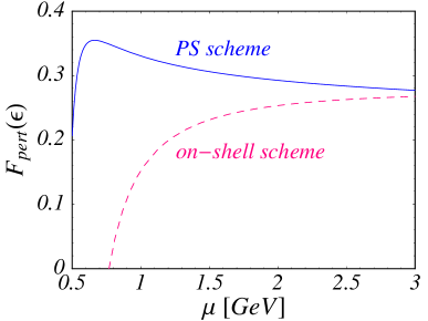
Figure 3: Scale dependence of the perturbative result for the fraction $F(\epsilon)$ to leading order in the hybrid expansion, evaluated for $q_{0}^{2}=(M_{B}-M_{D})^{2}$. The two curves refer to different mass renormalization schemes.

The dashed line in Figure 3 shows the perturbative prediction for the fraction $F(\epsilon)$ at leading order in $\epsilon$, as a function of the renormalization scale. Here and below we use the two-loop expression for the running coupling constant normalized such that $\alpha_{s}(M_{Z})=0.118$. In accordance with relation (19) below we use $m_{b}=5.0$ GeV for the pole mass, noting that this value (and thus the normalization of the dashed curve) has a large uncertainty. Two observations are important. First, the scale dependence of the dashed curve is significant, and hence the result obtained with an appropriate choice of scale $\mu\approx\mu_{c}$ is much lower than that obtained with the naive choice $\mu=m_{b}$. Secondly, perturbation theory in the on-shell scheme breaks down at a scale not much less than the appropriate scale $\mu\approx\mu_{c}\approx 1$ GeV. We conclude that in the on-shell scheme there is a large perturbative uncertainty in the calculation of the coefficient $C_{0}(\epsilon)$, which is not apparent from the naive one-loop result. This conclusion is in contrast with the assumption made by BLL, that the perturbative uncertainty is negligible [14].

The breakdown of perturbation theory at a scale of order $\mu_{c}$ can be traced back to the large coefficient of the NLO correction proportional to $\alpha_{s}(\mu)$ in (17). We will now show that the size of this coefficient can be reduced significantly by adopting a more appropriate definition of the heavy-quark mass. So far we have worked in the on-shell scheme, where the mass is defined as the pole in the renormalized quark propagator, $m_{b}=m_{b}^{\rm pole}$. Since the pole mass is affected by IR renormalon ambiguities [28, 29], it is better to eliminate it from the final expressions for inclusive decay rates. If a new mass definition $m_{b}^{\prime}$ is introduced via $m_{b}^{\rm pole}=Z_{m}\,m_{b}^{\prime}$, it follows from (5) that

$$C_{0}^{\prime}(\epsilon^{\prime})=C_{0}^{\rm pole}(\epsilon^{\prime})\left[1+\frac{Z_{m}-1}{\epsilon^{\prime}}\,\frac{(1-2\epsilon^{\prime})(3-4\epsilon^{\prime})}{1-\epsilon^{\prime}}+\dots\right]\,,$$ (18)

where the prime on $\epsilon$ indicates that this parameter in sensitive to the definition of $m_{b}$. We observe that a multiplicative redefinition of $m_{b}$ with $Z_{m}(\alpha_{s})=1+O(\alpha_{s})$, such as the relation between the pole mass and the running mass defined in the $\overline{\rm MS}$ scheme, is not appropriate in our case, since it would lead to a contribution to $C_{0}^{\prime}(\epsilon^{\prime})$ that is enhanced by a factor of $\alpha_{s}/\epsilon^{\prime}$. This would upset the power counting in the hybrid expansion. We suggest instead to work with a short-distance mass subtracted at a scale $\mu_{f}$ of order $\mu_{c}$, which is the natural scale of our problem.

It is well known that the convergence of the perturbative series for near on-shell problems in heavy-quark physics can be largely improved by introducing low-scale subtracted quark masses, which have the generic property that they differ from the pole mass by an amount proportional to the subtraction scale $\mu_{f}$. Several such mass definitions exist and have been applied to various processes [30, 31, 32, 33]. To illustrate the point, we use the potential-subtracted (PS) mass $m_{b}^{\rm PS}(\mu_{f})$ introduced by Beneke [30] and evaluate it at the scale $\mu_{f}=\mu_{c}^{\rm PS}$. At NLO, the relation between the pole mass and the PS mass reads

$$m_{b}^{\rm pole}=m_{b}^{\rm PS}(\mu_{c}^{\rm PS})+\mu_{c}^{\rm PS}\,\frac{4\alpha_{s}(\mu)}{3\pi}\left\{1+\frac{\alpha_{s}(\mu)}{2\pi}\left[\beta_{0}\left(\ln\frac{\mu}{\mu_{c}^{\rm PS}}+\frac{11}{6}\right)-4\right]+\dots\right\}\,,$$ (19)

which is formally independent of the scale $\mu$ at which the coupling is renormalized. Note that the difference between the two mass definitions is a perturbative series multiplying the scale $\mu_{c}^{\rm PS}=\epsilon^{\rm PS}m_{b}^{\rm PS}$. At NLO in $\alpha_{s}$, it then follows from (18) that

$$C_{0}^{\rm PS}(\epsilon^{\rm PS}) = C_{0}^{\rm pole}(\epsilon^{\rm PS})\left[1+\frac{4\alpha_{s}(\mu)}{3\pi}\,\frac{\mu_{c}^{\rm PS}}{\epsilon^{\rm PS}m_{b}^{\rm PS}}\,\frac{(1-2\epsilon^{\rm PS})(3-4\epsilon^{\rm PS})}{1-\epsilon^{\rm PS}}\right]$$ (20)

$$= C_{0}^{\rm pole}(\epsilon^{\rm PS})\left[1+\frac{4\alpha_{s}(\mu)}{\pi}+O(\epsilon^{\rm PS})\right]\,.$$

From now on we will use the PS mass $m_{b}\equiv m_{b}^{\rm PS}(\mu_{c}^{\rm PS})$ in all our equations and omit the label “PS” on the quantities $m_{b}$, $\mu_{c}$ and $\epsilon$. Using (17) and adding the extra contribution proportional to $\alpha_{s}(\mu)$, we obtain

$$C_{0}^{\rm PS}(\epsilon)\simeq\left(\frac{\alpha_{s}(\mu)}{\alpha_{s}(m_{b})}\right)^{\frac{12}{25}}\left[1-0.71\,\frac{\alpha_{s}(m_{b})}{\pi}+\frac{\alpha_{s}(\mu)}{\pi}\left(0.63+2\ln\frac{\mu}{\mu_{c}}\right)\right]+O(\epsilon)\,.$$ (21)

The introduction of the PS mass has much reduced the size of the NLO correction. The result for the leading contribution to $C_{0}(\epsilon)$ in the PS scheme is shown by the solid line in Figure 3. It exhibits a better stability that in the on-shell scheme, and it is stable down to lower values of the renormalization scale.

The value of the PS mass at the scale $\mu_{2}=2$ GeV has been determined from a sum-rule analysis of the $b\bar{b}$ production cross section near threshold, with the result $m_{b}^{\rm PS}(2\,{\rm GeV})=(4.59\pm 0.08)$ GeV (corresponding to $\overline{m}_{b}(m_{b})=(4.25\pm 0.08)$ GeV in the $\overline{\rm MS}$ scheme) [34]. At NLO, we can use relation (19) to convert this into a value of the PS mass at the scale $\mu_{c}$. This gives the implicit equation

$$m_{b}^{\rm PS}(\mu_{c}) = m_{b}^{\rm PS}(\mu_{2})+\mu_{c}\,\frac{4\alpha_{s}(\mu_{2})}{3\pi}\left[\left(\frac{\mu_{2}}{\mu_{c}}-1\right)\left(1+\frac{203}{36}\,\frac{\alpha_{s}(\mu_{2})}{\pi}\right)-\frac{25}{6}\,\frac{\alpha_{s}(\mu_{2})}{\pi}\ln\frac{\mu_{2}}{\mu_{c}}\right]$$ (22)

$$\stackrel{{\scriptstyle!}}{{=}} \mu_{c}+\sqrt{\mu_{c}^{2}+q_{0}^{2}}\,,$$

from which we determine the scale $\mu_{c}$ and then the mass $m_{b}=m_{b}^{\rm PS}(\mu_{c})$. For example, we find $m_{b}\simeq 4.73$ GeV, $\mu_{c}\simeq 1.13$ GeV, $\epsilon\simeq 0.24$ for $q_{0}^{2}=(M_{B}-M_{D})^{2}$, and $m_{b}\simeq 4.79$ GeV, $\mu_{c}\simeq 0.83$ GeV, $\epsilon\simeq 0.17$ for $q_{0}^{2}=15$ GeV².

In (21) we have obtained a RG-improved expression for the short-distance coefficient at leading order in $\epsilon$. It is at present not possible to extend this analysis to higher orders in the hybrid expansion, since the corresponding two-loop anomalous dimensions of higher-dimensional operators are unknown. However, since in the PS scheme the leading term in $\epsilon$ gives the dominant contribution to $C_{0}(\epsilon)$, we expect that the unresolved scale ambiguity in the higher-order terms does not introduce a large uncertainty. Our final expression for the short-distance coefficient at NLO is

$$C_{0}^{\rm PS}(\epsilon)\simeq\left(\frac{\alpha_{s}(\mu)}{\alpha_{s}(m_{b})}\right)^{\frac{12}{25}}\left[1-0.71\,\frac{\alpha_{s}(m_{b})}{\pi}+\frac{\alpha_{s}(\mu)}{\pi}\left(0.63+2\ln\frac{\mu}{\mu_{c}}\right)+\frac{\epsilon\bar{\alpha}_{s}}{\pi}\,G(\epsilon)\right]\,,$$ (23)

where the scale in $\bar{\alpha}_{s}$ in the $O(\epsilon)$ term remains undetermined. The exact result for the function $G(\epsilon)$ in the PS scheme is

$$G(\epsilon) = \frac{1}{12(1-\epsilon)\epsilon^{4}}\left[L_{2}(1-2\epsilon)-\frac{\pi^{2}}{6}-\left(\frac{13}{12}-8\epsilon+28\epsilon^{2}-\frac{128}{3}\epsilon^{3}+20\epsilon^{4}\right)\ln(1-2\epsilon)\right]$$ (24)

$$\mbox{}-\frac{1}{6(1-\epsilon)\epsilon^{3}}\left[\frac{1}{12}-\frac{89}{12}\epsilon+21\epsilon^{2}+40\epsilon^{3}-64\epsilon^{4}+\left(1+\epsilon+\frac{4}{3}\epsilon^{2}+2\epsilon^{3}\right)\ln 2\epsilon\right]$$

$$\mbox{}+\frac{4}{3\epsilon}\left[L_{2}(2\epsilon)-L_{2}(1-2\epsilon)+\frac{\pi^{2}}{6}\right]$$

$$= -\frac{8}{3}\ln 2\epsilon-\frac{95}{18}+\epsilon\left(-\frac{32}{15}\ln 2\epsilon+\frac{1337}{450}\right)+O(\epsilon^{2})\,.$$

The left-hand plot in Figure 4 shows $C_{0}(\epsilon)$ for the optimal choice $q_{0}^{2}=(M_{B}-M_{D})^{2}$ as a function of the renormalization scale. The width of the band reflects the sensitivity of the result to the value of the coupling $\bar{\alpha}_{s}$ associated with the $O(\epsilon)$ terms in (23), which we vary between $\alpha_{s}(m_{b})$ and $\alpha_{s}(\mu)$. To estimate the residual scale dependence we vary $\mu$ between the values $\mu_{c}$ and $2\mu_{c}$. For lower values the perturbative expansion diverges, since the running coupling $\alpha_{s}(\mu)$ strongly increases below $\mu\approx 1$ GeV. For comparison, we mention that the naive perturbative analysis with fixed scale $\mu=m_{b}$ adopted in [14] would give the much smaller value $C_{0}(\epsilon)\simeq 1.16$ at minimal $q_{0}^{2}\simeq 11.6$ GeV². The fact that we find larger QCD corrections will have important implications for the extraction of $|V_{ub}|$. The right-hand plot in Figure 4 shows $C_{0}(\epsilon)$ as a function of $q_{0}^{2}$. The width of the band represents the total scale uncertainty, estimated by variation of $\mu$ and $\bar{\alpha}_{s}$ as described above.

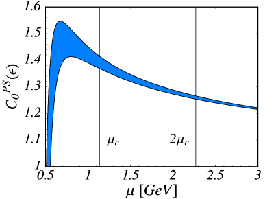
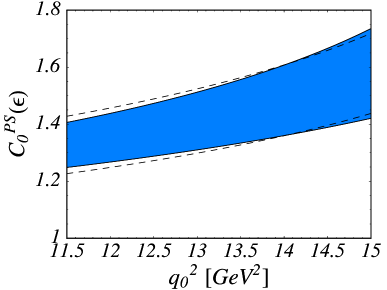
Figure 4: Left: Scale dependence of the coefficient $C_{0}^{\rm PS}(\epsilon)$ for $q_{0}^{2}=(M_{B}-M_{D})^{2}$. The width of the band indicates the scale ambiguity of higher-order terms in the hybrid expansion. The vertical lines show the window between $\mu=\mu_{c}$ and $\mu=2\mu_{c}$ used to estimate the scale dependence. Right: Coefficient $C_{0}(\epsilon)$ including theoretical uncertainties, as a function of the lepton invariant mass cut (see text).

An independent way to estimate the uncertainty in the value of the perturbative coefficient $C_{0}(\epsilon)$ is based on the contour representation (12) for the fraction $F(\epsilon)$. As we have just discussed, the value of $C_{0}(\epsilon)$ depends on the definition of the heavy-quark mass. However, the variation of the $O(\alpha_{s})$ correction in (13) along the circle in the complex momentum plane is independent of mass redefinitions. We may thus take the $\varphi$-variation of the one-loop correction, given by $\alpha_{s}(\mu_{c})/3\pi$ times the variation of the real part of the function $Y(e^{i\varphi},\epsilon)$ in (14), as a typical size of an $O(\alpha_{s})$ correction in the problem at hand. For an asymptotic series, the value of that correction provides an estimate for the magnitude of unknown higher-order corrections. The dashed lines in the right-hand plot in Figure 4 show this variation as an error band applied to the central values of $C_{0}(\epsilon)$. This independent evaluation of higher-order effects is in good agreement with our previous estimate of the perturbative uncertainty, giving us confidence that this estimate is a realistic one.

4 Higher-order power corrections

Uncertainties enter the theoretical prediction for the fraction $F(\epsilon)$ also at the level of power correction. First, there are unknown $O(\alpha_{s})$ corrections to the Wilson coefficient $C_{2}(\epsilon)$ multiplying the term proportional to $\lambda_{2}/\mu_{c}^{2}$ in (5). To estimate their effect, we replace the bracket $[\dots]$ in this equation with $C_{0}(\epsilon)\,[1-\frac{3}{2}\,C_{2}(\epsilon)\,\lambda_{2}/\mu_{c}^{2}+\dots]$, which amounts to multiplying the tree-level coefficient $C_{2}(\epsilon)$ in the original expression with $C_{0}(\epsilon)$. At $q_{0}=(M_{B}-M_{D})^{2}$, the difference is a $5\%$ effect. Potentially more important are higher-order power corrections scaling as $(\Lambda/\mu_{c})^{3}$. The operator matrix elements contributing at third order in the heavy-quark expansion can be identified [35, 36], but little is known about their actual size. Naive dimensional analysis suggests that, with a typical hadronic scale $\Lambda\approx 0.5$ GeV, a third-order power correction could be of order $(\Lambda/\mu_{c})^{3}\sim 0.09$ for $q_{0}^{2}=(M_{B}-M_{D})^{2}$ and $(\Lambda/\mu_{c})^{3}\sim 0.22$ for $q_{0}^{2}=15$ GeV², but clearly these are rough estimates which must be taken with caution.

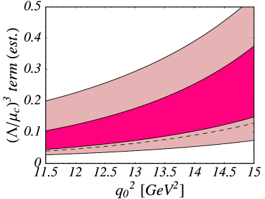
Figure 5: Estimates of third-order power corrections to the function $F(\epsilon)$, in units of the tree-level contribution (see text).

We will attempt to extract as much information about power corrections as possible from the formulae derived in Section 2 for the $B\to X\,l\,\nu$ decay rate and spectra in the presence of a lepton invariant mass cut. We start with the quantity $F(\epsilon)$ itself, which as shown in (5) receives a moderate second-order power correction proportional to the parameter $\lambda_{2}\simeq 0.12$ GeV². The dashed line in Figure 5 shows an estimate of the unknown $(\Lambda/\mu_{c})^{3}$ correction, obtained by raising this second-order term to the power 3/2. To address the question to what extent this is a conservative estimate of a “generic” higher-order correction, we focus on the differential spectrum in (10) and on the contour representation in (12). The function $F(\epsilon)$ is obtained from these results by performing integrals over $\xi$ or over the contour in the complex plane, respectively. However, the differential distributions contain additional information about power corrections, which is not seen after the integrations are performed. We first discuss the case of the contour integral in (12), taking the point of view that except for the region of small $\varphi$ the magnitude of $t(e^{i\varphi},\epsilon)$ can be used to estimate the “generic” size of corrections to the heavy-quark limit. This is so because on any point on the circle far away from the real, positive $\hat{p}^{2}$ axis, the function $t(e^{i\varphi},\epsilon)$ admits an operator product expansion in a series of local operators, whose contributions scale like powers of $\Lambda/\mu_{c}$. The average over the circle determines the corrections to the function $F(q_{0}^{2})$. However, the finer details of the distribution on the circle become relevant, e.g., when in a real experiment events with different hadronic masses and energies are weighted by different efficiencies. In other words, the various terms proportional to $\lambda_{1}/\mu_{c}^{2}$ and $\lambda_{2}/\mu_{c}^{2}$ in (13) are as valid as estimate of a second-order power correction as is the $\lambda_{2}/\mu_{c}^{2}$ term in (5). Specifically, we calculate the average value of the modulus of the power corrections in (13) on the circle in the complex plane, and then we raise this number to the power 3/2 to obtain an estimate of a “generic” $(\Lambda/\mu_{c})^{3}$ correction. For our numerical analysis we use $\lambda_{1}=-(0.30\pm 0.15)$ GeV², which is in the ball park of recent determinations [37]. The result is shown by the dark band in Figure 5, whose width reflects the sensitivity to the value of $\lambda_{1}$. If we were to consider larger values of $|\lambda_{1}|$ the upper limit of the band would increase. Another estimate of power corrections can be obtained from the coefficients of the various $\delta$-function terms in (10). If we take one third of the geometric average of the three coefficients, and raise the result to the power 3/2, we obtain the light band shown in the figure.

The above analysis shows that, as expected, there is a large uncertainty in the estimate of higher-order power corrections. We do not claim that these corrections are likely to be as large as indicated by the upper limit of the light band in Figure 5, however, as we have shown this would indeed be possible without introducing any unnaturally large coefficients or parameters. Keeping this caveat in mind, we will from now on use the upper limit of the dark band in the figure as our estimate of third-order power corrections. Numerically, this estimate is close to the one obtained by BLL [14].

5 Phenomenological implications and summary

The proposal of BLL is to use the theoretical calculation of the fraction $F(q_{0}^{2})$ to obtain a model-independent determination of the CKM matrix element $|V_{ub}|$ with controlled and small theoretical uncertainty [14]. To this end, one uses the relation ${\rm Br}(B\to X_{u}\,l\,\nu)|_{q^{2}>q_{0}^{2}}=F(q_{0}^{2})\,\Gamma(B\to X_{u}\,l\,\nu)\,\tau_{B}$, where $\tau_{B}$ is the $B$-meson lifetime, and $\Gamma(B\to X_{u}\,l\,\nu)$ is the total semileptonic decay rate into charmless final states. This rate can be calculated with high accuracy in terms of a low-scale subtracted $b$-quark mass, including perturbative corrections of order $[\alpha_{s}(m_{b})]^{2}$ [38] and power corrections of order $(\Lambda/m_{b})^{2}$. For our purposes, we use the PS mass defined at the scale $\mu_{2}=2$ GeV. Then the expression for the total rate is [33]

$$\Gamma(B\to X_{u}\,l\,\nu)=\frac{G_{F}^{2}|V_{ub}|^{2}[m_{b}^{\rm PS}(\mu_{2})]^{5}}{192\pi^{3}}\,(1+\delta_{\rm pert}+\delta_{\rm power})\,,$$ (25)

where $\delta_{\rm pert}\simeq 0.04$ at two-loop order, and $\delta_{\rm power}=\frac{\lambda_{1}-9\lambda_{2}}{2m_{b}^{2}}\simeq-0.03$. The small uncertainties in these two quantities are negligible for our numerical analysis below. Using these results, we obtain the master formula

$$|V_{ub}|=2.96\times 10^{-3}\left[\frac{{\rm Br}(B\to X\,l\,\nu)|_{q^{2}>q_{0}^{2}}}{10^{-3}\,F^{\prime}(q_{0}^{2})}\,\frac{1.6\,{\rm ps}}{\tau_{B}}\right]^{1/2},$$ (26)

where all theoretical uncertainties are contained in the function

$$F^{\prime}(q_{0}^{2})=\left(\frac{m_{b}^{\rm PS}(\mu_{2})}{4.59\,{\rm GeV}}\right)^{5}F(q_{0}^{2})\,.$$ (27)

The mass dependence due to factor $[m_{b}^{\rm PS}(\mu_{2})]^{5}$ from the total decay rate is positively correlated with the mass dependence of the function $F(q_{0}^{2})$. As a result, our predictions for the function $F^{\prime}(q_{0}^{2})$ become extremely sensitive to the value of the $b$-quark mass. For practical purposes, this dependence can be parameterized as

$$F^{\prime}(q_{0}^{2})\propto\left(\frac{m_{b}^{\rm PS}(\mu_{2})}{4.59\,{\rm GeV}}\right)^{\Delta(q_{0}^{2})},$$ (28)

where

$$\Delta(q_{0}^{2})\simeq 10+\frac{q_{0}^{2}-(M_{B}-M_{D})^{2}}{1\,\mbox{GeV}^{2}}\,.$$ (29)

In Table 1, we show our final results for the quantity $F^{\prime}(q_{0}^{2})$ and its theoretical uncertainties (as estimated above) for some representative values of $q_{0}^{2}$. For comparison, we note that BLL obtained the values $F^{\prime}((M_{B}-M_{D})^{2})=0.169\pm 0.016$ and $F^{\prime}(15\,{\rm GeV}^{2})=0.061\pm 0.013$, where the dominant theoretical error was assumed to be due to higher-order power corrections. Our central values are significantly higher because of the larger perturbative correction obtained after RG improvement. Note that our error estimates are about 2.5 times as large as those quoted by BLL. The difference between the central values of the two calculations is about $1\sigma$ of our errors, and about $2\sigma$ of their errors.

$\phantom{\bigg{|}}q_{0}^{2}\phantom{\bigg{|}}$	$F^{\prime}(q_{0}^{2})$	$\delta m_{b}$	$\alpha_{s}^{2}$	$\alpha_{s}(\Lambda/\mu_{c})^{2}$	$(\Lambda/\mu_{c})^{3}$
$\phantom{\bigg{|}}(M_{B}-M_{D})^{2}\phantom{\bigg{|}}$	$0.204\pm 0.040$	16.7%	6.0%	3.0%	8.2%
13 GeV2	$0.151\pm 0.036$	18.5%	7.2%	4.7%	12.5%
15 GeV2	$0.090\pm 0.032$	22.2%	10.0%	9.4%	23.8%

Table 1: Predictions for $F^{\prime}(q_{0}^{2})$ for three values of the lepton invariant mass cut. The right-hand portion contains the relative theoretical uncertainties due to the uncertainty in the value of the $b$-quark mass (assuming $\delta m_{b}=80$ MeV [34]), higher-order perturbative corrections (including scale dependence), perturbative corrections to second-order power corrections, and higher-order power corrections.

In Figure 6 we show a graphical representation of the fraction $F^{\prime}(q_{0}^{2})$ and its total theoretical uncertainty. This result, together with the master formula (26), provides the theoretical basis for the determination of $|V_{ub}|$. The right-hand plot in the figure shows the fractional theoretical uncertainty in the result for $|V_{ub}|$. Although our error estimates are more pessimistic than those presented by BLL, we still conclude that their method provides a very promising route for a precise determination of $|V_{ub}|$. For a realistic cut on the lepton invariant mass in the vicinity of $q_{0}^{2}\simeq 12.5$ GeV², which is about 1 GeV² above the optimal value, the theoretical uncertainty in $|V_{ub}|$ is close to 10%. A determination with such an accuracy would be a significant improvement with respect to the present knowledge of this important parameter. We believe it would also be more reliable than a future determination obtained by combining the partial decay rates in the endpoint regions of $B\to X_{s}\gamma$ and $B\to X_{u}\,l\,\nu$ decay spectra [6, 7, 8, 9], which is limited by uncontrollable power corrections of first order in $\Lambda/m_{b}$ that violate the factorization of soft and collinear singularities.

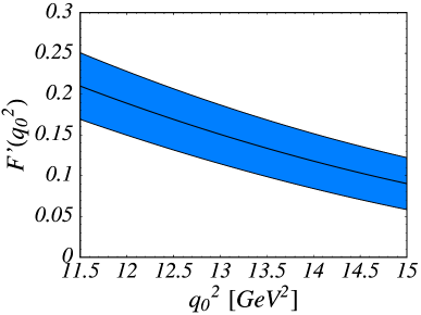
Figure 6: Left: Theoretical prediction for the quantity $F^{\prime}(q_{0}^{2})$. Right: Relative theoretical uncertainty in the extraction of $|V_{ub}|$.

According to Table 1, the dominant sources of theoretical uncertainty in the extraction of $|V_{ub}|$ are associated with the sensitivity to the value of the $b$-quark mass and with unknown, higher-order power corrections. Whereas it is not obvious how one should obtain a reliable value for the power corrections, the precision in the value of the $b$-quark mass can presumably be improved by reducing the theoretical uncertainties in the analysis of $(b\bar{b})$ bound states. In addition, it would be possible to reduce the perturbative uncertainty in the calculation in two ways, by calculating the exact $O(\alpha_{s}^{2})$ corrections to the fraction $F(q_{0}^{2})$ (the two-loop corrections to the total decay rate are known [38]), and by computing the two-loop anomalous dimensions of the operators contributing at $O(\epsilon)$ in the hybrid expansion. Both calculations are technically feasible and should be done.

In summary, we have analyzed the structure of the heavy-quark expansion for the inclusive, semileptonic $B\to X\,l\,\nu$ decay rate with a lepton invariant mass cut $q^{2}\geq q_{0}^{2}$. This expansion is characterized by a hadronic scale $\mu_{c}\ \hbox to0.0pt{\raise 3.0pt\hbox{$<$}\hss}{\lower 3.0pt\hbox{$\sim$}}\ m_{c}$ determined by the value of $q_{0}^{2}$. Because $m_{b}\gg\mu_{c}\gg\Lambda$, the heavy-quark expansion can be organized as a combined (hybrid) expansion in two small mass ratios. The physics associated with the two large scales $m_{b}$ and $\mu_{c}$ is disentangled using the HQET, whereas the physics on the scale $\mu_{c}$ can be separated from long-distance physics associated with $\Lambda$ utilizing an operator product expansion. We have used this formalism to obtain a RG-improved expression for the leading short-distance coefficient in the heavy-quark expansion at NLO. The summation of large logarithms in the hybrid expansion turns out to be important and strongly enhances the overall size of the perturbative correction. We have also emphasized that in order to obtain a stable perturbative prediction it is important to eliminate the $b$-quark pole mass in favor of a low-scale subtracted quark mass, such as the PS mass. Finally, we have presented several independent estimates of higher-order power corrections in the heavy-quark expansion, which at present do not permit a rigorous treatment. We find that with realistic values of the lepton invariant mass cut the overall theoretical uncertainty in the extraction of $|V_{ub}|$ is about 10%, which is larger than previously estimated but still significantly less than the current uncertainty in this parameter.