Back reaction of a long range force on a Friedmann-Robertson-Walker background
Abstract
It is possible that there may exist long-range forces in addition to gravity. In this paper we construct a simple model for such a force based on exchange of a massless scalar field and analyze its effect on the evolution of a homogeneous Friedmann-Robertson-Walker cosmology. The presence of such an interaction leads to an equation of state characterized by positive pressure and to resonant particle production similar to that observed in preheating scenarios.
98.80.Cq,04.62.+v,98.80.Hw
I Introduction
In nature, all forces except gravity seem to be restricted in range, either by an intrinsic range for the interaction, as in the case of the weak force, or by absence of free charges, as in the case of electromagnetism. There is, however, no physical principle which rules out the existence of a very weak long-range force in addition to gravity. String theory, for example, allows for massless scalars which could in principle be carriers of an additional force and which naturally would be long range. In order to be consistent with experiments such as solar system tests of general relativity and tests of the equivalence principle[1, 2], such an additional force must be either suppressed at short distances, much weaker than gravity at all scales, or must be decoupled from baryonic matter altogether. The latter possibility is particularly interesting given that the nature of cosmological dark matter is currently unknown. An extremely weak self interaction in dark matter is a distinct possibility, and short-range self interaction has been invoked in the literature to explain the discrepancy between observed and simulated dark matter profiles in galactic halos[3, 4, 5, 6, 7, 8, 9, 10, 11, 12]. If an additional long range force existed, it could significantly modify our understanding of the physics of galactic scales and larger[13, 14, 15, 16], but it may also affect the cosmology as a whole. It is the latter influence that we study here.
It has long been known that the equation of state of a thermodynamic system will be modified by interactions, for instance in the case of intermolecular forces in a gas. On cosmological level, a change in equation of state can be expected to produce a change in the evolution of background cosmology. In a cosmological context, unlike in a more conventional thermodynamic scenario, we wish to address what happens if the interaction is very long (if not infinite) range where relativistic effects become important. Therefore the proper treatment of this problem requires a relativistic formulation. For this purpose, we construct a simple example of a long range interaction in a Lorentz invariant field theoretic formulation, in particular a massive scalar field coupled to a massless scalar field which acts as a force carrier. We study the evolution of these fields in the background induced by themselves, and the evolution of the background (i.e the scale factor).
In addition to the virtue of simplicity, the zero mode of a massive scalar provides a reasonable model for cosmological matter, since in the noninteracting limit a massive scalar behaves very much like a pressureless dust. (For recent work on the possibility that dark matter could be a scalar field, see Refs. [7, 10, 11, 17, 18, 19, 20, 21, 22, 23].) An interaction will modify the stress-energy tensor of the cosmological matter, and thus can be expected to alter the evolution of the background cosmology.
The paper is organized as follows. First we introduce our model of a long range interaction, deliberately ignoring contact terms in order to emphasize that we are primarily interested in the effects of the long range component of the interaction. Then we study free massive scalar field in its own background, the behavior of the (incomplete) theory with the massless scalar exchange, and finally the full model included contact terms. We find the time evolution of fields, energy density and pressure, and the Hubble parameter in these cases.
Our conclusions are presented in the last section.
II Scalar long range force
Our model Lagrangian is:
| (1) | |||||
| (2) |
where is the scalar field of mass , is the massless force carrier, is the coupling (with dimension of mass), and . denotes the potential including the mass term.
In what follows, we will consider only the zero momentum states since we are interested in the long range effects. Obviously, the Lagrangian (2) is not a complete effective theory for the zero modes. Specifically, there are two marginal operators, and that should be included. ( which is also marginal, if generated by the interaction, would be suppressed compared to the other two marginal operators by two explicit additional powers of the coupling.) The marginal operators become important when the fields become large, and will be addressed later.
The full action of our model is
| (3) |
where is the Ricci scalar, is Newton’s constant, and The stress energy tensor is
| (4) |
We assume that the fields are dependent only on time, and that the background spacetime is a flat FRW cosmology. We use conformal coordinates, where is the scale factor, and is the conformal time. Then is diagonal,
| (5) |
where
| (6) | |||
| (7) |
The action implies the following coupled equations of motion for the fields , , and the scale factor :
| (8) | |||
| (9) | |||
| (10) |
where
| (11) |
denotes derivative with respect to the conformal time . It is convenient to introduce a dimensionless time , and rescale the fields to absorb :
| (12) | |||||
| (13) | |||||
| (14) |
The system of the coupled differential equations (10) then reads
| (15) | |||
| (16) | |||
| (17) |
Where an overdot denotes derivatives with respect to , and the rescaled energy density is defined as
| (18) |
We solve these equations numerically, subject to boundary conditions. We choose boundary conditions such that the force field, , is only virtual (i.e. ), that is, there is no radiation because we are only interested in the effect of the force itself. The source field, , is set to be at its free value initially, and is normalized by the requirement that .
A Free scalar field in its own background
In order to see how the long range force affects the time evolution of the system, it is of course necessary to first consider the case of the free field , i.e. and at all times.
At late times, the free field produces a background which is close, but not equal to, that of a pressureless dust ( with ). It can be seen from the following: Consider time evolution of a scalar field not in its own background but in the background produced by a dust with . (Recall that the scale factor and .) The equation of motion (17) of the field in this background,
| (19) |
can be solved analytically, leading to
| (20) |
where we choose the boundary conditions in such a way that is monotonic, and is a constant. With the background fixed as , consistent with our assumption of , the left hand side of the Friedmann equation is
| (21) |
If the solution (20) is to be self-consistent, this must be equal to the energy density , given by
| (22) |
We can normalize the field by fixing the scaling ambiguity in ,
| (23) |
so that
| (24) |
and setting gives
| (25) |
The energy density of the free scalar field agrees with the energy density of a pressureless dust up to corrections of . This observation is useful for two reasons. First, it shows that for numerical purposes it is convenient to choose the initial time because in that case, the analytical solution (20) is close to the exact solution for the noninteracting field. Thus it provides a good boundary condition for the interacting theory if the interaction is switched on at the time . Second, it allows for an independent check of the interacting theory via a perturbation theory with the lowest order given by the analytical solution in the background.
The analytical solution in the fixed background indicates a presence of small pressure, of order . In the full theory, there is indeed a small pressure but it is oscillatory and consistent with zero. The time evolution of the energy density is close to . (See Figures 5 and 6.) Nevertheless, the scale factor grows slightly more slowly than it would in the strictly pressureless case.
B The interacting case without the marginal operators
To understand the effect of the long range exchange itself, let us first consider the interaction without the marginal terms and . In this case we set up a perturbation theory to estimate time evolution of the fields and the scale factor. To do so, we note that the box operator (11) is easily inverted in the case where all spatial derivatives vanish:
| (26) | |||||
| (27) |
The fields and can be determined order by order in from their respective equations of motion, (17). By our choice of boundary conditions, the field starts at zeroth order, which we approximate by the analytical solution (20), while the field starts at order .
To leading order in , the equations of motion for the fields are
| (28) |
We take (Eq. 23). The field is then given by the the fixed background solution (20). The equation of motion for is
| (29) |
with solution
| (30) | |||||
| (31) |
The corrections to are , and those to are . To extend the perturbation expansion to higher order, it is necessary to include perturbations to the evolution of the scale factor. This can be accomplished self-consistently.
The field monotonically increases, despite the overall damping provided by the ever increasing scale factor. Numerical simulations confirm this observation. Note also that the presence of a horizon in the FRW space does not save us from a singularity as we take .
The behavior of the field can be simply understood. The boundary condition is zero field strength, , and from this point the field strength gradually builds up as more and more of the uniform source falls within the past light cone. This continues until the point at which it is possible for the virtual quanta to pair-produce real quanta of the field . This occurs when the potential energy, i.e. becomes equal the mass term . At this point the vacuum becomes unstable and the and fields rapidly pump one another. In the limit that , the fields are increasing very rapidly, and we can ignore the expansion term, and write the equations of motion as
| (32) | |||
| (33) |
from which we can derive a simple relation for the field strengths,
| (34) |
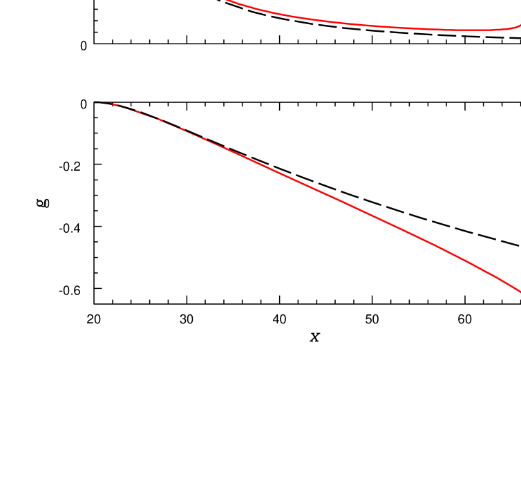
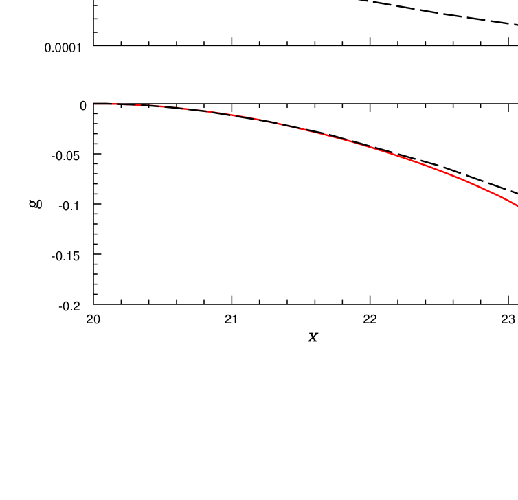
Therefore the fields grow without bound as , a behavior which is observed in the numerical solution. (Remarkably, our simple perturbation theory underestimates the field at the onset of the instability by only 20%.) This relationship between the field strengths has a simple interpretation in terms of particle number. Since the number densities are proportional to the square of the field strength, , an interaction of the form produces twice as many quanta of as quanta of . Figure 1 shows the the exact numerical solutions for the fields and compared to the free analytical solution (20), and the lowest order perturbative expression (31), respectively, for . The approximate solutions agree very well with the numerical results until very close to the onset of the instability. The plot of shows particularly distinctly the sharp rise of the field at the onset of the instability.
One would expect the approximate perturbative solutions and (20), (31) to break down in the limit of strong coupling, . In practice, the perturbative expressions work very well not only for weak coupling , but for relatively large as well. Figure 3 shows the fields and compared to the approximate solutions (20) and (31) for . Note that at the onset of instability the field is again underestimated by only 20% (as for ). The onset of instability is seen in both and .
This analysis, however, neglects one very important effect: the field is not only coupled to the zero mode of , but it is also coupled to modes with nonzero momentum. For a mode with dimensionless momentum , the equation of motion is:
| (35) |
The field can pair produce modes when
| (36) |
so that as grows, more and more phase space is populated through pair production. A proper treatment of particle production in this circumstance should invoke non-equilibrium dynamics, and is beyond the scope of our simple calculation. Similar systems have been studied in the literature [24, 25].
When the fields become large, however, the long range force is no longer the dominant factor. The contact interactions and become important. The instability is unphysical.
C Including the marginal operators
To stabilize the potential,
| (37) |
that is to make it bound from below, we now add the even marginal operators mentioned earlier. For our purposes, their coefficients are a priori unknown, because we use this model as an effective theory. In principle, the coefficients could be derived by integrating out degrees of freedom in the process of deriving the effective theory from the full theory at a different scale.
There are three marginal and even operators:
This operator by itself is sufficient to make the potential bound from below, providing its coupling is large enough. The potential (37) with this operator can be rewritten as follows:
| (38) |
which shows that has to be less than one, or else the minimum of the potential would be negative infinity at , and . In other words, the interaction decreases the mass of the . If the marginal operator is too weak the effective mass of becomes tachyonic as the field flows to its minimum.
Neither one of these operators alone can stabilize the potential. allows for potential to be unbound for , finite; and allows for finite, and . The sum of these two operators would make the potential to have a finite minimum. However, we have argued that the operator , if generated by a interaction, would have to be suppressed compared to the other two marginal operators and by two additional powers of coupling of the interaction. ( and can be expected to be of the same order.) For this reason, and in order to reduce number of parameters, we use only and . Further, for simplicity we assume that both these operators have the same coefficients. (This is a reasonable assumption if these operators arise from exchange of high energy or , respectively.) The qualitative features of the results are the same for unequal couplings as well.
The potential including the marginal operators is
| (39) |
where
| (40) |
The minimum of this potential is always finite, regardless of the value of and . If , or equivalently, , the absolute minimum of the potential is zero, at and . The case corresponds to a “broken” phase, similar to a “Mexican hat” potential. The potential still has a local extremum equal zero at and , but the absolute minimum is at , and it is negative, . The energy density can become negative. To make the theory consistent, one must add a constant to the potential so that the energy density is positive definite.
The numerical results that we present here were generated using the potential (39) in the unbroken phase. Even though the broken phase might seem like a better choice to represent the effect of the long range force because the marginal operators can be made arbitrarily weak, we find that it is less convenient for numerical reasons. In addition, we wish to avoid the presence of inflationary solutions. The results that we show are representative of a number of calculations with various couplings.
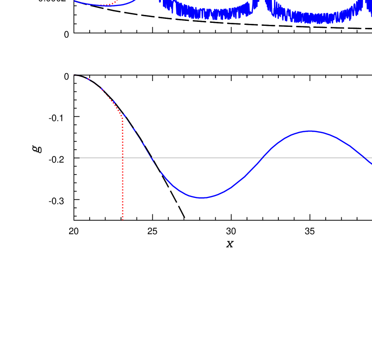
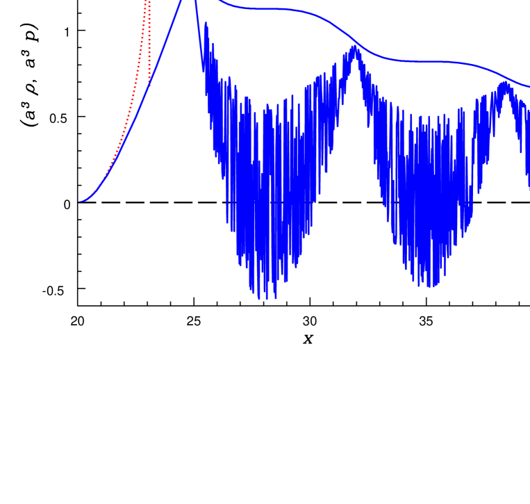
The evolution of the fields is at first identical to the case with no marginal operators because the long range component is dominating the physics (see Figure 3). The onset of the rapid growth of the fields in the presence of the marginal operators, Eq. (39), is delayed, compared to the onset of instability discussed in previous section, Eq. (37). Another difference between the two cases is that with the marginal operators, the field reaches its maximum and then starts oscillating. This is reminiscent of parametric particle production in preheating[26], and in fact similar. The difference is that in our case it is the energy stored in the massless messenger field that causes the peaks in the massive field . The parameters in the calculation shown in Figure 3 are chosen such that the field has a very small effective mass when reaches ; however the peaks in the field persist even if the mass is not close to zero. They do become wider and less steep with the increasing effective mass.
The plots also show the perturbative approximations for the fields and . The field is well approximated by the perturbative expression up until the growth of slows down and eventually ceases due to the marginal operators. Subsequently, is seen to oscillate around the value . The peaks in field occur when , that is the point in the potential valley when the effective mass is minimal. The field is also close to its free value until the onset of the instability. After that, in addition to rapid oscillations of the amplitude that are absent in the free case, the fully interacting field decreases more slowly than the free field.
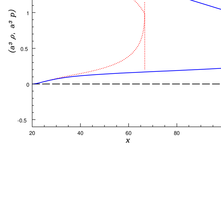
Next we show energy density and pressure. The long range force gives rise to a positive pressure, as can be expected from an attractive interaction. In the absence of marginal operators, the instability occurs when the pressure becomes equal to the energy density. At that point, the energy density drops to zero while pressure continues to grow and the theory becomes non-causal, . (Indeed, the field is effectively tachyonic.) This is just an indication that our “effective theory” for the long range force, consisting of just the relevant operator, is incomplete. When the marginal operators are included, the pressure builds up slower, and when it becomes equal to the energy density, it decreases and starts oscillating, following the behavior of the field. The energy density decreases monotonically, but it has saddle points.
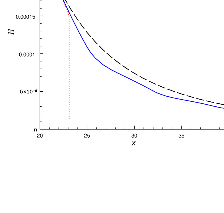
Although the behavior of the interacting matter differs markedly from the free theory, the effect on Hubble parameter is at most about 20% (Figure 5). This is partially because we start at time when the scale factor is already large.
The Hubble parameter for the free field is practically indistinguishable from the Hubble parameter due to a pressureless dust. In the case of the interacting theory with no marginal operators, the Hubble parameter is close to that of the free field, and then drops (to zero) when the instability occurs. This could be expected since the energy density is dropping also. With the marginal operators, the Hubble parameter is still monotonic, but it has saddle points at times when the amplitude of field peaks and field is equal , coinciding with the saddle points of the energy density. The rapid oscillations of are too fast to affect the Hubble parameter.At the first saddle point, the difference between the Hubble parameter of the free vs. interacting field is about 20%.
III Conclusion
In this paper we analyze a simple model for a long-range interaction in cosmological matter, based on exchange of a massless scalar “messenger” field . The boundary conditions are set such that the interaction is turned on at a finite time in a background consisting of the pressureless zero mode of a massive scalar field in a flat Friedmann-Robertson-Walker spacetime. We assume an interaction of the form . This coupling creates a negative interaction potential for the matter field, which, if not regulated by marginal operators in the Lagrangian, results in an unstable vacuum. The instability has a simple physical interpretation: the messenger field gradually builds in strength until the energy density in the field is large enough to pair-produce real matter particles. The particle production results in further strengthening of the messenger field and feedback results in strong pumping of both the matter and the messenger field. Since the potential is unbounded from below, this feedback continues indefinitely (Figs. 1 and 2). We observe that the matter field rapidly becomes tachyonic and the theory is non-causal, with pressure exceeding the energy density. With the addition of marginal operators of the form , and , the potential is bounded from below and the theory is well-defined. The early-time behavior of the theory is the same regardless of the presence of the marginal operators, but at late times the messenger field enters an oscillatory phase, resulting in resonant particle production in the matter field, similar to that seen in preheating scenarios (Fig. 3). We analyze the effect of the interaction on the equation of state of the cosmological matter and find that it results in the generation of an oscillating positive pressure term, with a maximum at (Figs. 5 and 6). This has two effects on the expansion. First, it results in an overall slowing of the expansion rate by a factor of about 20%. Second, the oscillations in the equation of state result in a deviation of the Hubble parameter from a simple power-law dependence on the conformal time (Fig 4).
The interaction we study here is mediated by a scalar and thus represents an attractive force. This is the simplest case, but potentially not the most interesting. A repulsive interaction, for instance one mediated by a vector field, could potentially provide a model for the mysterious “quintessence” responsible for the observed accelerating expansion of the universe. This is the subject of continuing study.
Acknowledgments
We would like to thank Dallas Kennedy and Richard Woodard for helpful conversations. This work was supported in part by U.S. D.O.E grant DE-FG02-97ER-41029.
REFERENCES
- [1] R. V. Eötvös, D. Pekár, E. Fekete, Ann. Physik 68, 11 (1922).
- [2] C. M. Will, Theory and Experiment in Gravitaional Physics (Cambridge University Press, Cambridge, 1993).
- [3] D. N. Spergel and P. J. Steinhardt, astro-ph/9909386.
- [4] S. Hannestad, astro-ph/9912558.
- [5] C. J. Hogan and J. J. Dalcanton, astro-ph/0002330.
- [6] A. Burkert, astro-ph/0002409.
- [7] P. J. E. Peebles, astro-ph/0002495.
- [8] J. Goodman, astro-ph/0003018.
- [9] S. Hannestad and R. J. Scherrer, astro-ph/0003046.
- [10] W. Hu, R. Barkana, and A. Gruzinov, astro-ph/0003365.
- [11] A. Riotto and I. Tkachev, astro-ph/0003388.
- [12] M. Kaplinghat, L. Knox, and M. S. Turner, astro-ph/0005210.
- [13] J. A. Frieman and B. Gradwohl, Phys. Rev. Lett 67, 2926 (1991).
- [14] B. Gradwohl and J. A. Frieman, Astrophys. J. 398, 407, (1992).
- [15] J. M. Gelb, B. Gradwohl, and J. A. Frieman, Astrophys. J. Lett. 403, L5 (1993), hep-ph/9208239.
- [16] W. H. Kinney and M. Brisudova, in preparation.
- [17] I. Zlatev and P. J. Steinhardt, astro-ph/9906481.
- [18] M. C. Bento and O. Bertolami, astro-ph/0003350.
- [19] T. Matos and L. A. Urenã-López, astro-ph/0004332.
- [20] T. Matos and L. A. Urenã-López, astro-ph/0006024.
- [21] W. Hu and P. J. E. Peebles, astro-ph/9910222.
- [22] V. Sahni and L. Wang, astro-ph/9910097.
- [23] T. Matos, F. S. Guzman, and L. A. Urenã-López, astro-ph/9908152.
- [24] D. Boyanovsky, H. J. de Vega, R. Holman, D. -S. Lee, and A. Singh, Phys. Rev. D 51, 4419 (1995), hep-ph/9408214.
- [25] D. Boyanovsky, H. J. de Vega, R. Holman, A. Singh, and M. Srednicki, Phys. Rev. D 56, 1939 (1997), hep-ph/9703327.
- [26] For a review, see L. Kofman, A. Linde, and A. A. Starobinsky, Phys. Rev. D 56, 3258 (1997), hep-ph/9704452.