$D^{*}D\pi$ and $B^{*}B\pi$ form factors from QCD Sum Rules

Abstract

The $H^{*}H\pi$ form factor for $H=B$ and $D$ mesons is evaluated in a QCD sum rule calculation. We study the Borel sum rule for the three point function of two pseudoscalar and one vector meson currents up to order four in the operator product expansion. The double Borel transform is performed with respect to the heavy meson momenta. We discuss the momentum dependence of the form factors and two different approaches to extract the $H^{*}H\pi$ coupling constant.
PACS numbers 14.40.Lb,  14.40.Nd,  12.38.Lg,  11.55.Hx

The coupling of the pion to the heavy mesons ($g_{B^{*}B\pi}$ and $g_{D^{*}D\pi}$) is related to the form factor at zero pionic momentum and its precise value has been often needed in phenomenology. In particular, the $g_{D^{*}D\pi}$ coupling is needed in the context of quark gluon plasma (QGP) physics. Suppression of charmonium production in heavy ion collisions is one of the signatures of QGP formation [1]. Therefore a precise evaluation of the background, i.e., conventional $J/\psi$ absorption by co-moving pions and $\rho$ mesons [2], is of fundamental importance. Since pions are so abundant in a dense nuclear environment, the reactions $\pi\,+\,J/\psi\,\rightarrow\,D\,+\,\overline{D^{*}}$ (and consequently the coupling $g_{D^{*}D\pi}$) are of special relevance [3].

In the case of $g_{D^{*}D\pi}$, the ${D^{*}}^{+}\rightarrow D^{0}\pi^{+}$ decay is observed experimentally. However, present data provide only an upper bound: $g_{D^{*}D\pi}\leq 21$ [4]. For $g_{B^{*}B\pi}$, there cannot be a direct experimental indication because there is no phase space for the $B^{*}\rightarrow B\pi$ decay. Recently, a direct preliminary determination of $g_{B^{*}B\pi}$ on the lattice has been attempted [5].

The $D^{*}D\pi$ and $B^{*}B\pi$ couplings have been studied by several authors using different approaches of the QCD sum rules (QCDSR): two point function combined with soft pion techniques [6, 7], light cone sum rules [8, 9], light cone sum rules including perturbative corrections [10], sum rules in a external field [11], double momentum sum rules [12]. Unfortunately, the numerical results from these calculations may differ by almost a factor two.

In this work we use the three-point function approach to evaluate the $D^{*}D\pi$ and $B^{*}B\pi$ form factors and coupling constants. The advantage of using the three-point function approach with a double Borel transformation compared with the two-point function with a single Borel transformation is the elimination of the terms associated with the pole-continuum transitions [8, 13].

The three-point function associated with a $H^{*}H\pi$ vertex, where $H$ and $H^{*}$ are respectively the lowest pseudoscalar and vector heavy mesons, is given by

$$\Gamma_{\mu}(p,p^{\prime})=\int d^{4}x\,d^{4}y\,\langle 0|T\{j(x)j_{5}(y)j^{\dagger}_{\mu}(0)\}|0\rangle\,e^{ip^{\prime}.x}\,e^{-i(p^{\prime}-p).y}\;,$$ (1)

where $j=i\bar{Q}\gamma_{5}u$, $j_{5}=i\bar{u}\gamma_{5}d$ and $j^{\dagger}_{\mu}=\bar{d}\gamma_{\mu}Q$ are the interpolating fields for $H$, $\pi^{-}$ and $H^{*}$ respectively with $u$, $d$ and $Q$ being the up, down, and heavy quark fields.

The phenomenological side of the vertex function, $\Gamma_{\mu}(p,p^{\prime})$, is obtained by the consideration of $H$ and $H^{*}$ state contribution to the matrix element in Eq. (1):

$$\Gamma_{\mu}^{(phen)}(p,p^{\prime}) = {1\over p^{2}-m_{H^{*}}^{2}}{1\over{p^{\prime}}^{2}-m_{H}^{2}}\langle 0|j|H(p^{\prime})\rangle\times$$ (3)

$$\langle H(p^{\prime})|j_{5}|H^{*}(p,\epsilon)\rangle\langle H^{*}(p,\epsilon)|j^{\dagger}_{\mu}|0\rangle+\mbox{higher resonances}\;.$$

The matrix element of the pseudoscalar element, $j_{5}$, defines the vertex form factor $g_{H^{*}H\pi}(q^{2})$:

$$\langle H(p^{\prime})|j_{5}|H^{*}(p,\epsilon)\rangle={f_{\pi}m_{\pi}^{2}\over m_{u}+m_{d}}{g_{H^{*}H\pi}(q^{2})\over q^{2}-m_{\pi}^{2}}q_{\nu}\epsilon^{\nu}\;,$$ (4)

where $q=p^{\prime}-p$, $f_{\pi}$ is the pion decay constant and $\epsilon^{\nu}$ is the polarization of the vector meson. The vacuum to meson transition amplitudes appearing in Eq. (3) are given in terms of the corresponding meson decay constants $f_{H}$ and $f_{H^{*}}$ by

$$\langle 0|j|H(p^{\prime})\rangle={m_{H}^{2}f_{H}\over m_{Q}}\;,$$ (5)

and

$$\langle H^{*}(p,\epsilon)|j^{\dagger}_{\mu}|0\rangle=m_{H^{*}}f_{H^{*}}\epsilon^{*}_{\mu}\;.$$ (6)

Therefore, using Eqs. (4), (5) and (6) in Eq. (3) we get

$$\Gamma_{\mu}^{(phen)}(p,p^{\prime}) = C_{HH^{*}}{g_{H^{*}H\pi}(q^{2})\over q^{2}-m_{\pi}^{2}}{1\over p^{2}-m_{H^{*}}^{2}}{1\over{p^{\prime}}^{2}-m_{H}^{2}}\times$$ (8)

$$\left(-p^{\prime}_{\mu}+{m_{H^{*}}^{2}+m_{H}^{2}-q^{2}\over 2m_{H^{*}}^{2}}p_{\mu}\right)+\mbox{higher resonances}\;,$$

where

$$C_{HH^{*}}={m_{H}^{2}m_{H^{*}}m_{\pi}^{2}f_{H}f_{H^{*}}f_{\pi}\over(m_{u}+m_{d})m_{Q}}\;.$$ (9)

The contribution of higher resonances and continuum in Eq. (8) will be taken into account as usual in the standard form of ref. [14].

The QCD side, or theoretical side, of the vertex function is evaluated by performing Wilson’s operator product expansion (OPE) of the operator in Eq. (1). Writing $\Gamma_{\mu}$ in terms of the invariant amplitudes:

$$\Gamma_{\mu}(p,p^{\prime})=\Gamma_{1}(p^{2},{p^{\prime}}^{2},q^{2})p_{\mu}+\Gamma_{2}(p^{2},{p^{\prime}}^{2},q^{2})p^{\prime}_{\mu}\;,$$ (10)

we can write a double dispersion relation for each one of the invariant amplitudes $\Gamma_{i}\,(i=1,2)$, over the virtualities $p^{2}$ and ${p^{\prime}}^{2}$ holding $Q^{2}=-q^{2}$ fixed:

$$\Gamma_{i}(p^{2},{p^{\prime}}^{2},Q^{2})=-{1\over 4\pi^{2}}\int_{m_{Q}^{2}}^{\infty}ds\int_{m_{Q}^{2}}^{\infty}du{\rho_{i}(s,u,Q^{2})\over(s-p^{2})(u-{p^{\prime}}^{2})}\;,$$ (11)

where $\rho_{i}(s,u,Q^{2})$ equals the double discontinuity of the amplitude $\Gamma_{i}(p^{2},{p^{\prime}}^{2},Q^{2})$ on the cuts $m_{Q}^{2}\leq s\leq\infty$, $m_{Q}^{2}\leq u\leq\infty$, which can be evaluated using Cutkosky’s rules [14, 15].

Finally we perform a double Borel transformation [14] in both variables $P^{2}=-p^{2}$ and ${P^{\prime}}^{2}=-{p^{\prime}}^{2}$ and equate the two representations described above. We get one sum rule for each invariant function. In the $p_{\mu}$ structure:

$$-C_{HH^{*}}{m_{H^{*}}^{2}+m_{H}^{2}+Q^{2}\over 2m_{H^{*}}^{2}}{g_{H^{*}H\pi}(q^{2})\over Q^{2}+m_{\pi}^{2}}e^{-m_{H^{*}}^{2}/M^{2}}e^{-m_{H}^{2}/{{M^{\prime}}^{2}}} = -{1\over 4\pi^{2}}\int_{m_{Q}^{2}}^{s_{0}}ds\int_{m_{Q}^{2}}^{u_{0}}du\left[\right.$$ (13)

$$\left.\rho_{1}(s,u,Q^{2})e^{-s/M^{2}}e^{-u/{M^{\prime}}^{2}}\right]\;,$$

and in the $p^{\prime}_{\mu}$ structure:

$$C_{HH^{*}}{g_{H^{*}H\pi}(q^{2})\over Q^{2}+m_{\pi}^{2}}e^{-m_{H^{*}}^{2}/M^{2}}e^{-m_{H}^{2}/{{M^{\prime}}^{2}}}=-{1\over 4\pi^{2}}\int_{m_{Q}^{2}}^{s_{0}}ds\int_{m_{Q}^{2}}^{u_{0}}du\left[\rho_{2}(s,u,Q^{2})e^{-s/M^{2}}e^{-u/{M^{\prime}}^{2}}\right]\;,$$ (14)

where $s_{0}$ and $u_{0}$ are the continuum thresholds for the $H^{*}$ and $H$ mesons respectively, which are, in general, taken from the mass sum rules. The two Borel masses $M^{2}$ and ${M^{\prime}}^{2}$ are, in principle, independent and they should vary in the vicinity of the corresponding meson masses: $m_{H^{*}}^{2}$ and $m_{H}^{2}$ respectively. Since for heavy mesons $m_{H}$ and $m_{H^{*}}$ are very close, many authors use $M^{2}={M^{\prime}}^{2}$ [8, 10, 11]. To allow for different values of $M^{2}$ and ${M^{\prime}}^{2}$ we take them proportional to the respective meson masses, which leads us to study the sum rule as a function of $M^{2}$ at a fixed ratio

$${M^{2}\over{M^{\prime}}^{2}}={m_{H^{*}}^{2}\over m_{H}^{2}}\;.$$ (15)

We will consider diagrams up to dimension four which include the perturbative diagram and the gluon condensate. The quark condensate term does not contribute since it depends only on one external momentum and, therefore, it is eliminated by the double Borel transformation. Higher dimension condensates are strongly suppressed in the case of heavy quarks [6, 7, 8, 9, 11, 12]. The double discontinuity of the perturbative contribution reads:

$$\rho_{1}^{(pert)}(s,u,Q^{2})=-{3Q^{2}u(2m_{Q}^{2}-s-u-Q^{2})\over[(s+u+Q^{2})^{2}-4su]^{3/2}}\;,$$ (16)

$$\rho_{2}^{(pert)}(s,u,Q^{2})={3Q^{2}[m_{Q}^{2}(s+u+Q^{2})-2su]\over[(s+u+Q^{2})^{2}-4su]^{3/2}}\;,$$ (17)

and the integration limit condition is

$$(s-m_{Q}^{2})(u-m_{Q}^{2})\geq Q^{2}m_{Q}^{2}\;.$$ (18)

In this paper we focus on the structure $p_{\mu}$ which we found to be the more stable one. For consistency we use in our analysis the QCDSR expressions for the decay constants up to dimension four in lowest order of $\alpha_{s}$:

$$f_{H}^{2}={3m_{Q}^{2}\over 8\pi^{2}m_{H}^{4}}\int_{m_{Q}^{2}}^{u_{0}}du{(u-m_{Q}^{2})^{2}\over u}e^{(m_{H}^{2}-u)/{M^{\prime}}^{2}}\,-\,{m_{Q}^{3}\over m_{H}^{4}}\langle\bar{q}q\rangle e^{(m_{H}^{2}-m_{Q}^{2})/{M^{\prime}}^{2}}\;,$$ (19)

$$f_{H^{*}}^{2}={1\over 8\pi^{2}m_{H^{*}}^{2}}\int_{m_{Q}^{2}}^{s_{0}}ds{(s-m_{Q}^{2})^{2}\over s}\left(2+{m_{Q}^{2}\over s}\right)e^{(m_{H^{*}}^{2}-s)/M^{2}}\,-\,{m_{Q}\over m_{H^{*}}^{2}}\langle\bar{q}q\rangle e^{(m_{H^{*}}^{2}-m_{Q}^{2})/M^{2}}\;,$$ (20)

where we have omitted the numerically insignificant contribution of the gluon condensate.

The parameter values used in all calculations are $m_{u}+m_{d}=14\,\nobreak\,\mbox{MeV}$, $m_{c}=1.5\,\nobreak\,\mbox{GeV}$, $m_{b}=4.7\,\nobreak\,\mbox{GeV}$, $m_{\pi}=140\,\nobreak\,\mbox{MeV}$, $m_{D}=1.87\,\nobreak\,\mbox{GeV}$, $m_{D^{*}}=2.01\,\nobreak\,\mbox{GeV}$, $m_{B}=5.28\,\nobreak\,\mbox{GeV}$, $m_{B^{*}}=5.33\,\nobreak\,\mbox{GeV}$, $f_{\pi}=131.5\,\nobreak\,\mbox{MeV}$, $\langle\overline{q}q\rangle\,=\,-(0.23)^{3}\,\nobreak\,\mbox{GeV}^{3}$, $\langle g^{2}G^{2}\rangle=0.5\,\nobreak\,\mbox{GeV}^{4}$. We parametrize the continuum thresholds as

$$s_{0}=(m_{H^{*}}+\Delta_{s})^{2}\;,$$ (21)

and

$$u_{0}=(m_{H}+\Delta_{u})^{2}\;.$$ (22)

The values of $u_{0}$ and $s_{0}$ are, in general, extracted from the two-point function sum rules for $f_{H}$ and $f_{H*}$ in Eqs. (19) and (20). Using the Borel region $2\leq M^{2}\leq 5\nobreak\,\mbox{GeV}^{2}$ (for the $D^{*}$ and $D$ mesons) and $10\leq M^{2}\leq 25\nobreak\,\mbox{GeV}^{2}$ (for the $B^{*}$, and $B$ mesons) we found a good stability for $f_{H}$ and $f_{H*}$ with $\Delta_{s}=\Delta_{u}\sim 0.5\nobreak\,\mbox{GeV}$, in agreement with the results in ref. [8]. We have checked that bigger values for $\Delta_{s(u)}$, of order of 1 GeV, lead to unstable results for $f_{H}$ and $f_{H*}$, in the case of the sum rules Eqs. (19) and (20). In our study we will allow for a small variation in $\Delta_{s}$ and $\Delta_{u}$ to test the sensitivity of our results to the continuum contribution.

We first discuss the $D^{*}D\pi$ form factor. In Fig. 1 we show the behavior of the perturbative and gluon condensate contributions to the form factor $g_{D^{*}D\pi}(Q^{2})$ at $Q^{2}=1\,\nobreak\,\mbox{GeV}$ as a function of the Borel mass $M^{2}$ using $\Delta_{s}$ and $\Delta_{u}$ given in Eqs. (21) and (22) equal to $0.5\,\nobreak\,\mbox{GeV}$. We can see that, in the case of the form factor, the gluon condensate is not negligible and it helps the stability of the curve, as a function of $M^{2}$, providing a rather stable plateau for $M^{2}\geq 3\,\nobreak\,\mbox{GeV}^{2}$. The behavior of the curve for other $Q^{2}$ and continuum treshold values is similar. Fixing $M^{2}=3.5\,\nobreak\,\mbox{GeV}^{2}$ we show, in Fig. 2, the momentum dependence of the form factor (dots). Since the present approach cannot be used at $Q^{2}=0$, to extract the $g_{D^{*}D\pi}$ coupling from the form factor we need to extrapolate the curve to $Q^{2}=0$ (in the approximation $m_{\pi}^{2}=0$). In order to do this extrapolation we fit the QCD sum rule results (dots) with an analytical expression. We tried to fit our results with a monopole form, since this is very often used for form factors, but the fit is very poor. We obtained good fits using both the gaussian form

$$g_{H^{*}H\pi}(Q^{2})=g_{H^{*}H\pi}\,e^{-(Q^{2}+m_{\pi}^{2})^{2}/\Gamma^{4}}$$ (23)

and a curve of the form

$$g_{H^{*}H\pi}(Q^{2})=g_{H^{*}H\pi}{1+(a/\Lambda)^{4}\over 1+(a/\Lambda)^{4}e^{(Q^{2}+m_{\pi}^{2})^{2}/\Lambda^{4}}}\;.$$ (24)

In Fig. 2 we show that the $Q^{2}$ dependence of the form factor, represented by the dots, can be well reproduced by the parametrization in Eqs. (23) (dashed line) and (24) (solid line). The value of the parameters in Eqs. (23) and (24) are given in Table I for two different values of the continuum threshold.

$\Delta_{s}=\Delta_{u}\,(\nobreak\,\mbox{GeV})$	$g_{D^{*}D\pi}$	$\Lambda\,(\nobreak\,\mbox{GeV})$	$a\,(\nobreak\,\mbox{GeV})$	$\Gamma\,(\nobreak\,\mbox{GeV})$
0.5	5.3	1.66	1.90	-
0.6	6.0	1.89	3.05	-
0.5	5.7	-	-	1.74
0.6	6.1	-	-	1.92

TABLE I: Values of the parameters in Eqs. (23) and (24) which reproduce the QCDSR results for $g_{D^{*}D\pi}(Q^{2})$, for two different values of the continuum thresholds in Eqs. (21) and (22).

In view of the uncertainties involved, the results obtained with the two parametrizations are consistent with each other, the systematic error being of the order of $10\%$.

In refs. [8, 16] it was found that the form factor in the semileptonic decay $H\rightarrow\pi l\bar{\nu}$, which is also normalized by the $H^{*}H\pi$ coupling constant, can be well approximated by a monopole form factor. In the case of the $H\rightarrow\pi l\bar{\nu}$ form factor, a vector dominance approximation gives a phenomenological explanation for a pole fit at $q^{2}=m_{H^{*}}^{2}$, which is not the case of the form factor studied here. It is important to notice that here the dispersion relation is written in terms of the two heavy meson momenta, while in the case of semileptonic decay the dispersion relation is a function of the $H$ and $\pi$ momenta. Therefore, our form factor is a function of the pion momentum, exhibiting a peak at the pion pole $Q^{2}=0$.

To test if our fit gives a good extrapolation to $Q^{2}=0$ we can write a sum rule, based on the three-point function Eq. (1), but valid only at $Q^{2}=0$, as suggested in [17] for the pion-nucleon coupling constant. This method was also applied to the nucleon-hyperon-kaon coupling constant [18, 19] and to the nucleon$-\Lambda_{c}-D$ coupling constant [20]. It consists in neglecting the pion mass in the denominator of Eq. (8) and working at $Q^{2}=0$, making a single Borel transformation to both $P^{2}={P^{\prime}}^{2}\rightarrow M^{2}$.

As discussed in the introduction, the problem of doing a single Borel transformation is the fact that the single pole contribution, associated with the $N\rightarrow N^{*}$ transition, is not suppressed [6, 8, 13]. In ref. [13] it was explicitly shown that the pole-continuum transition has a different behavior as a function of the Borel mass as compared with the double pole contribution and continuum contribution: it grows with $M^{2}$ as compared with the double pole contribution. Therefore, the single pole contribution can be taken into account through the introduction of a parameter $A$, in the phenomenological side of the sum rule [8, 13, 19]. Thus, neglecting $m_{\pi}^{2}$ in the denominator of Eq. (8) and doing a single Borel transform in $P^{2}={P^{\prime}}^{2}$, we get for the structure $p_{\mu}$

$$\tilde{\Gamma}_{1}^{(phen)}(M^{2},Q^{2})=-{C_{H^{*}H}\over 2m_{H}^{2}Q^{2}}{m_{H}^{2}+m_{H^{*}}^{2}+Q^{2}\over m_{H^{*}}^{2}-m_{H}^{2}}\left(e^{-m_{H}^{2}/M^{2}}-e^{-m_{H^{*}}^{2}/M^{2}}\right)(g_{H^{*}H\pi}+AM^{2})\;,$$ (25)

where $C_{H^{*}H}$ in given in Eq. (9) with $f_{H}$ and $f_{H^{*}}$ given by Eqs. (19) and (20).

On the OPE side only terms proportional to $1/Q^{2}$ will contribute to the sum rule. Therefore, up to dimension four the only diagram that contributes is the quark condensate given by

$$\tilde{\Gamma}_{1}^{<\bar{q}q>}(M^{2},Q^{2})={2m_{Q}\langle\overline{q}q\rangle\over Q^{2}}\,e^{-m_{Q}^{2}/M^{2}}\;.$$ (26)

Equating Eqs. (25) and (26) and taking $Q^{2}=0$ we obtain the sum rule for $g_{H^{*}H\pi}+AM^{2}$, where $A$ denotes the contribution from the unknown single poles terms. It is interesting to point out that in the limit $m_{H}^{2}+m_{H^{*}}^{2}=2m_{H^{*}}^{2}$, the sum rule obtained in the $p^{\prime}_{\mu}$ structure coincides with the sum rule in the $p_{\mu}$ structure. In Fig. 3 we show, for $\Delta_{s}=\Delta_{u}=0.5\,\nobreak\,\mbox{GeV}$, the QCDSR results for $g_{D^{*}D\pi}+AM^{2}$ as a function of $M^{2}$ (dots) from where we see that, in the Borel region $2\leq M^{2}\leq 5\,\nobreak\,\mbox{GeV}^{2}$, they follow a straight line. The value of the coupling constant is obtained by the extrapolation of the line to $M^{2}=0$ [13]. Fitting the QCDSR results to a straight line we get

$$g_{D^{*}D\pi}\simeq 5.4\;,$$ (27)

in excellent agreement with the values obtained with the extrapolation of the form factor to $Q^{2}=0$, given in Table I.

It is reassuring that both methods, with completely different OPE sides and Borel transformation approaches, give the same value for the coupling constant.

In the case of $B^{*}B\pi$ vertex, we show in Fig. 4, for $\Delta_{s}=\Delta_{u}=0.5\,\nobreak\,\mbox{GeV}$, the $Q^{2}=0$ sum rule results for $g_{B^{*}B\pi}+AM^{2}$ (dots) as a function of $M^{2}$. It also follows a straight line in the Borel region $10\leq M^{2}\leq 25\,\nobreak\,\mbox{GeV}^{2}$, and the extrapolation to $M^{2}=0$ gives

$$g_{B^{*}B\pi}\simeq 10.6\;.$$ (28)

In Fig. 6 we show the QCDSR result for the perturbative and gluon condensate contributions to the form factor $g_{B^{*}B\pi}(Q^{2})$ at $Q^{2}=2\,\nobreak\,\mbox{GeV}^{2}$ as a function of $M^{2}$ using $\Delta_{s}=\Delta_{u}=0.5\,\nobreak\,\mbox{GeV}$. In this case the gluon condensate is very small but it still goes in the right direction of providing a stable plateau for $M^{2}\geq 15\,\nobreak\,\mbox{GeV}^{2}$. Fixing $M^{2}=17\,\nobreak\,\mbox{GeV}^{2}$ we show, in Fig. 6, the $Q^{2}$ behavior of the form factor (dots). The dots can still be well fitted by Eq. (24) (solid line). However, the fit with Eq. (23) is not so good, as can be seen by the dashed line in Fig. 6. In Table II we give the value of the parameters in Eqs. (23) and (24) that reproduce our results for two different choices of the continuum thresholds.

In this case the agreement of the two different approaches to extract the coupling constant is not so good, but the numbers are still compatible. One possible reason for that is the fact that for heavier quarks the perturbative contribution (or hard physics) becomes more important, as can be observed by the decrease of the importance of the gluon condensate in Fig. 5 as compared with Fig. 1. Since in the sum rule given by Eqs. (25) and (26) there is only soft physics information, we expect $\alpha_{s}$ corrections to the sum rule to be more important in the case of $g_{B^{*}B\pi}(Q^{2})$ than for $g_{D^{*}D\pi}(Q^{2})$.

$\Delta_{s}=\Delta_{u}\,(\nobreak\,\mbox{GeV})$	$g_{B^{*}B\pi}$	$\Lambda\,(\nobreak\,\mbox{GeV})$	$a\,(\nobreak\,\mbox{GeV})$	$\Gamma\,(\nobreak\,\mbox{GeV})$
0.5	14.7	1.62	1.37	-
0.6	16.3	1.81	1.67	-
0.5	17.2	-	-	1.79
0.6	18.4	-	-	1.97

TABLE II: Values of the parameters in Eqs. (23) and (24) which reproduce the QCDSR results for $g_{B^{*}B\pi}(Q^{2})$, for two different values of the continuum thresholds in Eqs. (21) and (22).

Comparing Table I with Table II we see that the cut-offs are of the same order in the two vertices and are very hard. Concerning the parameter $a$, it is smaller in the case of the $B^{*}B\pi$ vertex. This is because of the fact that the form factor $g_{B^{*}B\pi}(Q^{2})$ has a flatter peak around $Q^{2}=0$ than $g_{D^{*}D\pi}(Q^{2})$. This can be interpreted as an indication that the spatial extension of the vertex is smaller for $B^{*}B\pi$ than for $D^{*}D\pi$. This is also the reason why the gaussian fit is not so good in the case of the $B^{*}B\pi$ vertex, and leads to bigger values for the coupling. It is interesting to notice that our results for the coupling constants are completely consistent with the QCDSR calculation of ref. [12].

As a final exercise, we use our result for $g_{B^{*}B\pi}$ to extract the coupling constant $g$ which controls the interaction of the pion with infinitely heavy fields in effective lagrangian approaches [21, 22]. They are related by [6, 7, 8, 9, 11, 12, 21, 22]

$$g_{B^{*}B\pi}={2m_{B}\over f_{\pi}}g\;.$$ (29)

The knowledge of $g$ is of great phenomenological value, since its strenght is required in the analyzes of many electroweak processes [21]. Therefore, during the last years, a large number of theoretical papers has been devoted to the calculation of $g$. However, the variation of the value obtained for $g$, even within a single class of models, turns out to be quite large. For instance, using different quark models one obtains $1/3\leq g\leq 1$ [22, 23] while QCDSR calculations points in the direction of small $g$, with a typical value in the range $g\simeq 0.13-0.35$ [6, 7, 8, 9, 11, 12].

Using the values for $g_{B^{*}B\pi}$ given in Table II we get, at order $\alpha_{s}=0$

$$g=0.13-0.23\;,$$ (30)

therefore, we corroborate the overall conclusion drawn from different QCDSR calculations, that the coupling $g$ is small.

In conclusion, we extracted the $H^{*}H\pi$ coupling constant using two different approaches of the QCDSR based on the three-point function. We have obtained for the coupling constants:

$$g_{D^{*}D\pi}=5.7\pm 0.4\;,$$ (31)

$$g_{B^{*}B\pi}=14.5\pm 3.9\;,$$ (32)

where the errors reflect variations in the continuum thresholds, different parametrizations of the form factors and the use of two different sum rules. There are still sources of errors in the values of the condensates and in the choice of the Borel mass to extract the form factor, which were not considered here. Therefore, the errors quoted are probably underestimated.

In Table III we present a compilation of the estimates of the coupling constants $g_{D^{*}D\pi}$ and $g_{B^{*}B\pi}$ from distinct QCDSR calculations.

approach	$g_{D^{*}D\pi}$	$g_{B^{*}B\pi}$
this work	$5.7\pm 0.4$	$14.5\pm 3.9$
two-point function + soft pion techniques (2PFSP)[6]	$9\pm 2$	$20\pm 4$
2PFSP + perturbative corrections [6]	$7\pm 2$	$15\pm 4$
light cone sum rules (LCSR) [8]	$11\pm 2$	$28\pm 6$
LCSR + perturbative corrections [10]	$10.5\pm 3$	$22\pm 9$
double momentum sum rule [12]	$6.3\pm 1.9$	$14\pm 4$

TABLE III: Summary of QCDSR estimates for $g_{D^{*}D\pi}$ and $g_{B^{*}B\pi}$.

From this Table we see that our result is in a fair agreement with the calculations in refs. [6, 12], while LCSR calculations point to bigger values for the coupling constants. This discrepancy has still to be solved.

The $D^{*}D\pi$ coupling is directly related with the $D^{*}\rightarrow D\pi$ decay width through

$$\Gamma({D^{*}}^{-}\rightarrow{\overline{D^{0}}}\pi^{-})={g_{D^{*}D\pi}^{2}|\vec{q}_{\pi}|^{3}\over 24\pi m_{D^{*}}^{2}}\;.$$ (33)

Using Eq. (31) we get

$$\Gamma({D^{*}}^{-}\rightarrow{\overline{D^{0}}}\pi^{-})=6.3\pm 0.9\;\nobreak\,\mbox{keV}\;,$$ (34)

which is much smaller then the current upper limit [4] $\Gamma({D^{*}}^{-}\rightarrow{\overline{D^{0}}}\pi^{-})<89$ keV.

Acknowledgements: This work has been supported by CNPq and FAPESP (under project number 1998/2249-4). C.L.S. thanks FAPERJ for financial support.

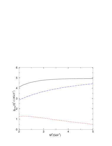
FIG. 1.: $M^{2}$ dependence of the perturbative (long-dashed line) and gluon condensate (dashed line) contributions to the $D^{*}D\pi$ form factor at $Q^{2}=1\,\nobreak\,\mbox{GeV}^{2}$ (solid line) for $\Delta_{s}=\Delta_{u}=0.5\,\nobreak\,\mbox{GeV}$.

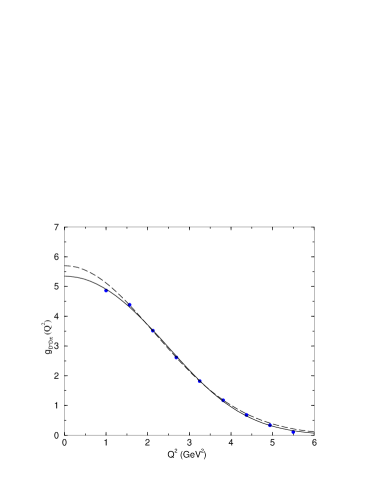
FIG. 2.: Momentum dependence of the $D^{*}D\pi$ form factor for $\Delta_{s}=\Delta_{u}=0.5\,\nobreak\,\mbox{GeV}$ (dots). The solid and dashed lines give the parametrization of the QCDSR results through Eqs. (24) and (23) respectively.

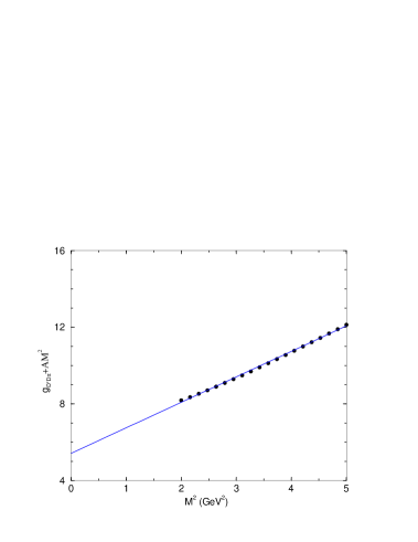
FIG. 3.: $D^{*}D\pi$ coupling constant as a function of the squared Borel mass $M^{2}$ from the QCDSR valid at $Q^{2}=0$ (dots). The straight line gives the extrapolation to $M^{2}=0$.

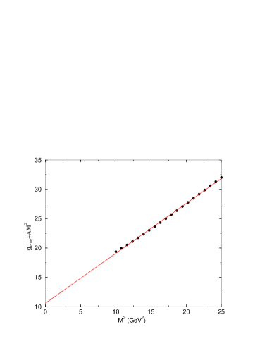
FIG. 4.: $B^{*}B\pi$ coupling constant as a function of the squared Borel mass $M^{2}$ from the QCDSR valid at $Q^{2}=0$ (dots).The straight line gives the extrapolation to $M^{2}=0$.

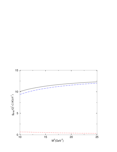
FIG. 5.: $M^{2}$ dependence of the perturbative (long-dashed line) and gluon condensate (dashed line) contributions to the $B^{*}B\pi$ form factor at $Q^{2}=2\,\nobreak\,\mbox{GeV}^{2}$ (solid line) for $\Delta_{s}=\Delta_{u}=0.5\,\nobreak\,\mbox{GeV}$.

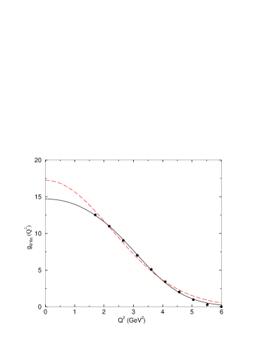
FIG. 6.: Momentum dependence of the $B^{*}B\pi$ form factor for $\Delta_{s}=\Delta_{u}=0.5\,\nobreak\,\mbox{GeV}$ (dots). The solid and dashed lines give the parametrization of the QCDSR results through Eqs. (24) and (23) respectively.