QCD

Abstract

We discuss issues of QCD at the LHC including parton distributions, Monte Carlo event generators, the available next-to-leading order calculations, resummation, photon production, small $x$ physics, double parton scattering, and backgrounds to Higgs production.

1 INTRODUCTION

It is well known that precision QCD calculations and their experimental tests at a proton–proton collider are inherently difficult. “Unfortunately”, essentially all physics aspects of the LHC, from particle searches beyond the Standard Model (SM) to electroweak precision measurements and studies of heavy quarks are connected to the interactions of quarks and gluons at large transferred momentum. An optimal exploitation of the LHC is thus unimaginable without the solid understanding of many aspects of QCD and their implementation in accurate Monte Carlo programs.

This review on QCD aspects relevant for the LHC gives an overview of today’s knowledge, of ongoing theoretical efforts and of some experimental feasibility studies for the LHC. More aspects related to the experimental feasibility and an overview of possible measurements, classified according to final state properties, can be found in Chapter 15 of Ref. [1]. It was impossible, within the time-scale of this Workshop, to provide accurate and quantitative answers to all the needs for LHC measurements. Moreover, owing to the foreseen theoretical and experimental progress, detailed quantitative studies of QCD will have necessarily to be updated just before the start of the LHC experimental program. The aim of this review is to update Ref. [2] and to provide reference work for the activities required in preparation of the LHC program in the coming years.

Especially relevant for essentially all possible measurements at the LHC and their theoretical interpretation is the knowledge of the parton (quark, anti-quark and gluon) distribution functions (pdf’s), discussed in Sect. 2. Today’s knowledge about quark and anti-quark distribution functions comes from lepton-hadron deep-inelastic scattering (DIS) experiments and from Drell-Yan (DY) lepton-pair production in hadron collisions. Most information about the gluon distribution function is extracted from hadron–hadron interactions with photons in the final state. The theoretical interpretation of a large number of experiments has resulted in various sets of pdf’s which are the basis for cross section predictions at the LHC. Although these pdf’s are widely used for LHC simulations, their uncertainties are difficult to estimate and various quantitative methods are being developed now (see Sects. $2.1-2.4$).

The accuracy of this traditional approach to describe proton–proton interactions is limited by the possible knowledge of the proton–proton luminosity at the LHC. Alternatively, much more precise information might eventually be obtained from an approach which considers the LHC directly as a parton–parton collider at large transferred momentum. Following this approach, the experimentally cleanest and theoretically best understood reactions would be used to normalize directly the LHC parton–parton luminosities to estimate various other reactions. Today’s feasibility studies indicate that this approach might eventually lead to cross section accuracies, due to experimental uncertainties, of about $\pm$ 1%. Such accuracies require that in order to profit, the corresponding theoretical uncertainties have to be controlled at a similar level using perturbative calculations and the corresponding Monte Carlo simulations. As examples, the one-jet inclusive cross section and the rapidity dependence of $W$ and $Z$ production are known at next-to-leading order, implying a theoretical accuracy of about 10 %. To improve further, higher order corrections have to be calculated.

Section 3 addresses the implementation of QCD calculations in Monte Carlo programs, which are an essential tool in the preparation of physics data analyses. Monte Carlo programs are composed of several building blocks, related to various stages in the interaction: the hard scattering, the production of additional parton radiation and the hadronization. Progress is being made in the improvement and extension of matrix element generators and in the prediction for the transverse momentum distribution in boson production. Besides the issues of parton distributions and hadronization, another non-perturbative piece in a Monte Carlo generator is the treatment of the minimum bias and underlying events. One of the important issue discussed in the section on Monte Carlo generators is the consistent matching of the various building blocks. More detailed studies on Monte Carlo generators for the LHC will be performed in a foreseen topical workshop.

The status of higher order calculations and prospects for further improvements are presented in Sect. 4. As mentioned earlier, one of the essential ingredients for improving the accuracy of theoretical predictions is the availability of higher order corrections. For almost all processes of interest, containing a (partially) hadronic final state, the next-to-leading order (NLO) corrections have been computed and allow to make reliable estimates of production cross sections. However, to obtain an accurate estimate of the uncertainty, the calculation of the next-to-next-to-leading order (NNLO) corrections is needed. These calculations are extremely challenging and once performed, they will have to be matched with a corresponding increase in accuracy in the evolution of the pdf’s.

Section 5 discusses the summations of logarithmically enhanced contributions in perturbation theory. Examples of such contributions occur in the inclusive production of a final-state system which carries a large fraction of the available center-of-mass energy (“threshold resummation”) or in case of the production of a system with high mass at small transverse momentum (“$p_{T}$ resummation”). In case of threshold resummations, the theoretical calculations for most processes of interest have been performed at next-to-leading logarithmic accuracy. Their importance is two-fold: firstly, the cross sections at LHC might be directly affected; secondly, the extraction of pdf’s from other reactions might be influenced and thus the cross sections at LHC are modified indirectly. For transverse momentum resummations, two analytical methods are discussed.

The production of prompt photons (as discussed in Sect. 6) can be used to put constraints on the gluon density in the proton and possibly to obtain measurements of the strong coupling constant at LHC. The definition of a photon usually involves some isolation criteria (against hadrons produced close in phase space). This requirement is theoretically desirable, as it reduces the dependence of observables on the fragmentation contribution to photon production. At the same time, it is useful from the experimental point of view as the background due to jets faking a photon signature can be further reduced. A new scheme for isolation is able to eliminate the fragmentation contribution.

In Sect. 7 the issue of QCD dynamics in the region of small $x$ is discussed. For semi-hard strong interactions, which are characterized by two large, different scales, the cross sections contain large logarithms. The resummation of these at leading logarithmic (LL) accuracy can be performed by the BFKL equation. Available experimental data are however not described by the LL BFKL, indicating the present of large sub-leading contributions and the need to include next-to-leading corrections. Studies of QCD dynamics in this regime can be made not only by using inclusive observables, but also through the study of final state properties. These include the production of di-jets at large rapidity separation (studying the azimuthal decorrelation between the two jets) or the production of mini-jets (studying their multiplicity).

An important topic at the LHC is multiple (especially double) parton scattering (described in Sect. 8), i.e. the simultaneous occurrence of two independent hard scattering in the same interaction. Extrapolations to LHC energies, based on measurements at the Tevatron show the importance of taking this process into account when small transverse momenta are involved. Manifestations of double parton scattering are expected in the production of four jet final states and in the production of a lepton in association with two $b$-quarks (where the latter is used as a final state for Higgs searches).

The last section (Sect. 9) addresses the issue of the present knowledge of background for Higgs searches, for final states containing two photons or multi-leptons. For the case of di-photon final states (used for Higgs searches with $90<m_{H}<140$ GeV), studies of the irreducible background are performed by calculating the (single and double) fragmentation contributions to NLO accuracy and by studying the effects of soft gluon emission. The production of rare five lepton final states could provide valuable information on the Higgs couplings for $m_{H}>200$ GeV, awaiting further studies on improving the understanding of the backgrounds.

During the workshop, no studies of diffractive scattering at the LHC have been performed. This topic is challenging both from the theoretical and the experimental point of view. The study of diffractive processes (with a typical signature of a leading proton and/or a large rapidity gap) should lead to an improved understanding of the transition between soft and hard process and of the non-perturbative aspects of QCD. From the experimental point of view, the detection of leading protons in the LHC environment is challenging and requires adding additional detectors to ATLAS and CMS. If hard diffractive scattering (leading proton(s) together with e.g. jets as signature for a hard scattering) is to be studied with decent statistical accuracy at large $p_{T}$, most of the luminosity delivered under normal running conditions has to be utilized. A few more details can be found in Chapter 15 of Ref. [1], some ideas for detectors in Ref. [3]. Much more work remains to be done, including a detailed assessment of the capabilities of the additional detectors.

1.1 Overview of QCD tools

All of the processes to be investigated at the LHC involve QCD to some extent. It cannot be otherwise, since the colliding quarks and gluons carry the QCD color charge. One can use perturbation theory to describe the cross section for an inclusive hard-scattering process,

$$h_{1}(p_{1})+h_{2}(p_{2})\rightarrow H(Q,\{\dots\})+X\;\;.$$ (1)

Here the colliding hadrons $h_{1}$ and $h_{2}$ have momenta $p_{1}$ and $p_{2}$, $H$ denotes the triggered hard probe (vector bosons, jets, heavy quarks, Higgs bosons, SUSY particles and so on) and $X$ stands for any unobserved particles produced by the collision. The typical scale $Q$ of the scattering process is set by the invariant mass or the transverse momentum of the hard probe and the notation $\{\dots\}$ stands for any other measured kinematic variable of the process. For example, the hard process may be the production of a $Z$ boson. Then $Q=M_{Z}$ and we can take $\{\dots\}=y$, where $y$ is the rapidity of the $Z$ boson. One can also measure the transverse momentum $Q_{T}$ of the the $Z$ boson. Then the simple analysis described below applies if $Q_{T}\sim M_{Z}$. In the cases $Q_{T}\ll M_{Z}$ and $M_{Z}\ll Q_{T}$, there are two hard scales in the process and a more complicated analysis is needed. The case $Q_{T}\ll M_{Z}$ is of particular importance and is discussed in Sects. 3.3, 3.4 and 5.3.

The cross section for the process (1) is computed by using the factorization formula [4, 5]

$$\sigma(p_{1},p_{2};Q,\{\dots\})\!\!\! = \!\!\!\sum_{a,b}\int dx_{1}\,dx_{2}\,f_{a/h_{1}}(x_{1},Q^{2})\,f_{b/h_{2}}(x_{2},Q^{2})\;{\hat{\sigma}}_{ab}(x_{1}p_{1},x_{2}p_{2};Q,\{\dots\};\alpha_{\mathrm{S}}(Q))$$ (2)

$$+ \!\!\!{\cal O}\left((\Lambda_{QCD}/Q)^{p}\right)\;\;.$$

Here the indices $a,b$ denote parton flavors, {$g,u,\bar{u},d,\bar{d},\dots$}. The factorization formula (2) involves the convolution of the partonic cross section ${\hat{\sigma}}_{ab}$ and the parton distribution functions $f_{a/h}(x,Q^{2})$ of the colliding hadrons. The term ${\cal O}\left((\Lambda_{QCD}/Q)^{p}\right)$ on the right-hand side of Eq. (2) generically denotes non-perturbative contributions (hadronization effects, multiparton interactions, contributions of the soft underlying event and so on).

Evidently, the pdf’s are of great importance to making predictions for the LHC. These functions are determined from experiments. Some of the issues relating to this determination are discussed in Sect. 2 In particular, there are discussions of the question of error analysis in the determination of the pdf’s and there is a discussion of the prospects for determining the pdf’s from LHC experiments.

The partonic cross section ${\hat{\sigma}}_{ab}$ is computable as a power series expansion in the QCD coupling $\alpha_{\mathrm{S}}(Q)$:

$$\!\!\!\!\!\!{\hat{\sigma}}_{ab}(p_{1},p_{2};Q,\{\dots\};\alpha_{\mathrm{S}}(Q))\!\!\!\! = \!\!\!\!\alpha_{\mathrm{S}}^{k}(Q)\left\{{\hat{\sigma}}_{ab}^{(LO)}(p_{1},p_{2};Q,\{\dots\})\right.$$ (3)

$$\;\;\;\;\;\;\;\;\;\;+\,\alpha_{\mathrm{S}}(Q)\;{\hat{\sigma}}_{ab}^{(NLO)}(p_{1},p_{2};Q,\{\dots\})$$

$$\;\;\;\;\;\;\;\;\;\;+\left.\!\alpha_{\mathrm{S}}^{2}(Q)\;{\hat{\sigma}}_{ab}^{(NNLO)}(p_{1},p_{2};Q,\{\dots\})+\cdots\right\}\,.$$

The lowest (or leading) order (LO) term ${\hat{\sigma}}^{(LO)}$ gives only a rough estimate of the cross section. Thus one needs the next-to-leading order (NLO) term, which is available for most cases of interest. A list of the available calculations is given in Sect. 4.1. Cross sections at NNLO are not available at present, but the prospects are discussed in Sect. 4.2.

The simple formula (2) applies when the cross section being measured is “infrared safe.” This means that the cross section does not change if one high energy strongly interacting light particle in the final state divides into two particles moving in the same direction or if one such particle emits a light particle carrying very small momentum. Thus in order to have a simple theoretical formula one does not typically measure the cross section to find a single high-$p_{T}$ pion, say, but rather one measures the cross section to have a collimated jet of particles with a given total transverse momentum $p_{T}$. If, instead, a single high-$p_{T}$ pion (or, more generally, a high-$p_{T}$ hadron $H$) is measured, the factorization formula has to include an additional convolution with the corresponding parton fragmentation function $d_{a/H}(z,Q^{2})$. An example of a case where one needs a more complicated treatment is the production of high-$p_{T}$ photons. This case is discussed in Sect. 6

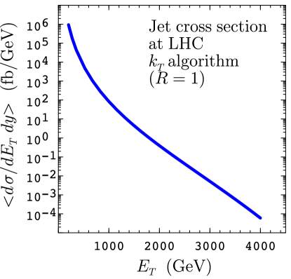
Figure 1: Jet cross section at the LHC, averaged over the rapidity interval $-1<y<1$. The cross section is calculated at NLO using CTEQ5M partons with the renormalization and factorization scales set to $\mu_{R}=\mu_{F}=E_{T}/2$. Representative values at $E_{T}=$0.5, 1, 2, 3 and 4 TeV are $(6.2\times 10^{3},8.3\times 10^{1},4.0\times 10^{-1},5.1\times 10^{-3},5.9\times 10^{-5})$ fb/GeV with about 3% statistical errors.

As an example of a NLO calculation, we display in Fig. 1 the predicted cross section $d\sigma/dE_{T}\,dy$ at the LHC for the inclusive production of a jet with transverse energy $E_{T}$ and rapidity $y$ averaged over the rapidity interval $-1<y<1$. The calculation uses the program in Ref. [6] and the pdf set CTEQ5M [7]. As mentioned above, the “jets” must be defined with an infrared safe algorithm. Here we use the $k_{T}$ algorithm [8, 9] with a joining parameter $R=1$. The $k_{T}$ algorithm has better theoretical properties than the cone algorithm that has often been used in hadron collider experiments.

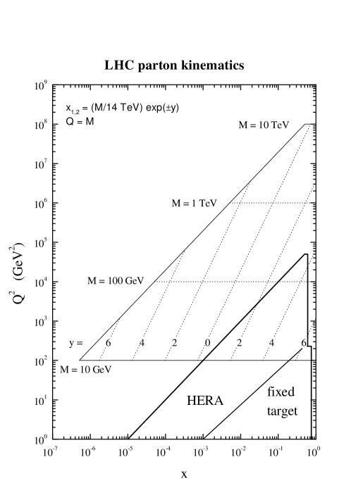
Figure 2: Values of $x$ and $Q^{2}$ probed in the production of an object of mass $M$ and rapidity $y$ at the LHC, $\sqrt{s}=14$ TeV.

In Eq. (2) there are integrations over the parton momentum fractions $x_{1}$ and $x_{2}$. The values of $x_{1}$ and $x_{2}$ that dominate the integral are controlled by the kinematics of the hard-scattering process. In the case of the production of a heavy particle of mass $M$ and rapidity $y$, the dominant values of the momentum fractions are $x_{1,2}\sim(Me^{\pm y})/{\sqrt{s}}$, where $s=(p_{1}+p_{2})^{2}$ is the square of the centre-of-mass energy of the collision. Thus, varying $M$ and $y$ at fixed ${\sqrt{s}}$, we are sensitive to partons with different momentum fractions. Increasing ${\sqrt{s}}$ the pdf’s are probed in a kinematic range that extends towards larger values of $Q$ and smaller values of $x_{1,2}$. This is illustrated in Fig. 2. At the LHC, $x_{1,2}$ can be quite small. Thus small $x$ effects that go beyond the simple formula (2) could be important. These are discussed in Sect. 7

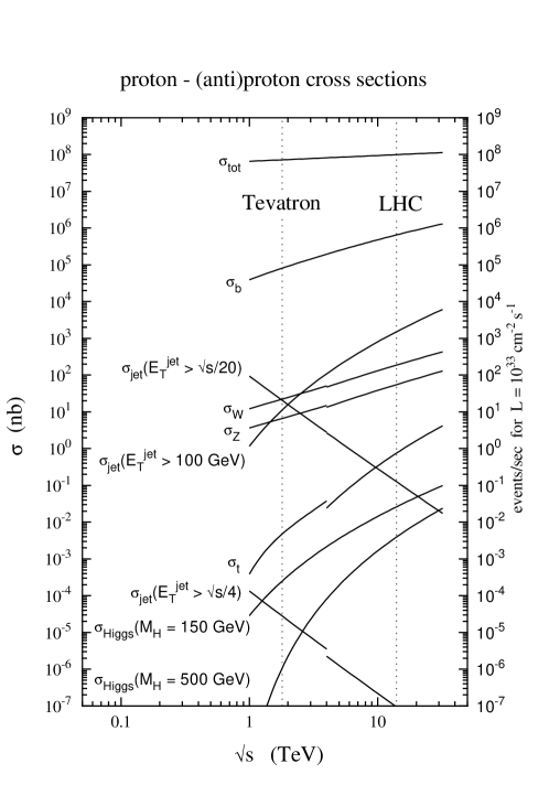
Figure 3: Cross sections for hard scattering versus $\sqrt{s}$. The cross section values at $\sqrt{s}=14$ TeV are: $\sigma_{\rm tot}=99.4$ mb, $\sigma_{\rm b}=0.633$ mb, $\sigma_{\rm t}=0.888$ nb, $\sigma_{\rm W}=187$ nb, $\sigma_{\rm Z}=55.5$ nb, $\sigma_{{\rm H}}(M_{\rm H}=150\;{\rm GeV})=23.8$ pb, $\sigma_{{\rm H}}(M_{\rm H}=500\;{\rm GeV})=3.82$ pb, $\sigma_{{\rm jet}}(E_{T}^{\rm jet}>100\;{\rm GeV})=1.57\;\mu$b, $\sigma_{{\rm jet}}(E_{T}^{\rm jet}>\sqrt{s}/20)=0.133$ nb, $\sigma_{{\rm jet}}(E_{T}^{\rm jet}>\sqrt{s}/4)=0.10$ fb. All except the first of these are calculated using the latest MRST pdf’s [10].

In Fig. 3 we plot NLO cross sections for a selection of hard processes versus $\sqrt{s}$. The curves for the lower values of $\sqrt{s}$ are for $p\bar{p}$ collisions, as at the Tevatron, while the curves for the higher values of $\sqrt{s}$ are for $pp$ collisions, as at the LHC. An approximation (based on an extrapolation of a standard Regge parametrization) to the total cross section is also displayed. We see that the cross sections for production of objects with a fixed mass or jets with a fixed transverse energy $E_{T}$ rise with $\sqrt{s}$. This is because the important $x_{1,2}$ values decrease, as discussed above, and there are more partons at smaller $x$. On the other hand, cross sections for jets with transverse momentum that is a fixed fraction of $\sqrt{s}$ fall with $\sqrt{s}$. This is (mostly) because the partonic cross sections $\hat{\sigma}$ fall with $E_{T}$ like $E_{T}^{-2}$.

The perturbative evaluation of the factorization formula (2) is based on performing power series expansions in the QCD coupling $\alpha_{\mathrm{S}}(Q)$. The dependence of $\alpha_{\mathrm{S}}$ on the scale $Q$ is logarithmic and it is given by the renormalization group equation [4]

$$Q^{2}\frac{d\alpha_{\mathrm{S}}(Q)}{dQ^{2}}=\beta(\alpha_{\mathrm{S}}(Q))=-b_{0}\,\alpha_{\mathrm{S}}^{2}(Q)-b_{1}\,\alpha_{\mathrm{S}}^{3}(Q)+\cdots\;\;,$$ (4)

where the first two perturbative coefficients are

$$b_{0}=\frac{33-2N_{f}}{12\pi}\;\;,\quad b_{1}=\frac{153-19N_{f}}{24\pi^{2}}\;\;,$$ (5)

and $N_{f}$ is the number of flavours of light quarks (quarks whose mass is much smaller than the scale $Q$). The third and fourth coefficients $b_{2}$ and $b_{3}$ of the $\beta$-function are also known [11, 12]. If we include only the LO term, Eq. (4) has the exact analytical solution

$$\alpha_{\mathrm{S}}(Q)=\frac{1}{b_{0}\ln(Q^{2}/\Lambda_{QCD}^{2})}\;\;,$$ (6)

where the integration constant $\Lambda_{QCD}$ fixes the absolute size of the QCD coupling. From Eq. (6) we can see that a change of the scale $Q$ by an arbitrary factor of order unity (say, $Q\rightarrow Q/2$) induces a variation in $\alpha_{\mathrm{S}}$ that is of the order of $\alpha_{\mathrm{S}}^{2}$. This variation in uncontrollable because it is beyond the accuracy at which Eq. (6) is valid. Therefore, in LO of perturbation theory the size of $\alpha_{\mathrm{S}}$ is not unambiguously defined.

The QCD coupling $\alpha_{\mathrm{S}}(Q)$ can be precisely defined only starting from the NLO in perturbation theory. To this order, the renormalization group equation (4) has no exact analytical solution. Different approximate solutions can differ by higher-order corrections and some (arbitrary) choice has to be made. Different choices can eventually be related to the definition of different renormalization schemes. The most popular choice [13] is to use the $\overline{\mbox{\rm{\small{MS}}}}$-scheme to define renormalization and then to use the following approximate solution of the two loop evolution equation to define $\Lambda_{QCD}$:

$$\alpha_{\mathrm{S}}(Q)=\frac{1}{b_{0}\ln(Q^{2}/\Lambda_{\overline{\mbox{\rm{\small{MS}}}}}^{2})}\left[1-\frac{b_{1}\ln\big{[}\ln(Q^{2}/\Lambda_{\overline{\mbox{\rm{\small{MS}}}}}^{2})\big{]}}{b_{0}\ln(Q^{2}/\Lambda_{\overline{\mbox{\rm{\small{MS}}}}}^{2})}+{\cal O}\!\left(\frac{\ln^{2}\big{[}\ln(Q^{2}/\Lambda_{\overline{\mbox{\rm{\small{MS}}}}}^{2})\big{]}}{\ln^{2}(Q^{2}/\Lambda_{\overline{\mbox{\rm{\small{MS}}}}}^{2})}\right)\right]\;\;.$$ (7)

Here the definition of $\Lambda_{QCD}$ $(\Lambda_{QCD}=\Lambda_{\overline{\mbox{\rm{\small{MS}}}}})$ is contained in the fact that there is no term proportional to $1/\ln^{2}(Q^{2}/\Lambda_{QCD}^{2})$. In this expression there are $N_{f}$ light quarks. Depending on the value of $Q$, one may want to use different values for the number of quarks that are considered light. Then one must match between different renormalization schemes, and correspondingly change the value of $\Lambda_{\overline{\mbox{\rm{\small{MS}}}}}$ as discussed in Ref. [13]. The constant $\Lambda_{\overline{\mbox{\rm{\small{MS}}}}}$ is the one fundamental constant of QCD that must be determined from experiments. Equivalently, experiments can be used to determine the value of $\alpha_{\mathrm{S}}$ at a fixed reference scale $Q=\mu_{0}$. It has become standard to choose $\mu_{0}=M_{Z}$. The most recent determinations of $\alpha_{\mathrm{S}}$ lead [13] to the world average $\alpha_{\mathrm{S}}(M_{Z})=0.119\pm 0.002$. In present applications to hadron collisions, the value of $\alpha_{\mathrm{S}}$ is often varied in the wider range $\alpha_{\mathrm{S}}(M_{Z})=0.113-0.123$ to conservatively estimate theoretical uncertainties.

The parton distribution functions $f_{a/h}(x,Q^{2})$ at any fixed scale $Q$ are not computable in perturbation theory. However, their scale dependence is perturbatively controlled by the DGLAP evolution equation [14, 15, 16, 17]

$$Q^{2}\frac{d\,f_{a/h}(x,Q^{2})}{dQ^{2}}=\sum_{b}\int_{x}^{1}\frac{dz}{z}\,P_{ab}(\alpha_{\mathrm{S}}(Q^{2}),z)\,f_{a/h}(x/z,Q^{2})\;\;.$$ (8)

Having determined $f_{a/h}(x,Q_{0}^{2})$ at a given input scale $Q=Q_{0}$, the evolution equation can be used to compute the pdf’s at different perturbative scales $Q$ and larger values of $x$.

The kernels $P_{ab}(\alpha_{\mathrm{S}},z)$ in Eq. (8) are the Altarelli–Parisi (AP) splitting functions. They depend on the parton flavours $a,b$ but do not depend on the colliding hadron $h$ and thus they are process-independent. The AP splitting functions can be computed as a power series expansion in $\alpha_{\mathrm{S}}$:

$$P_{ab}(\alpha_{\mathrm{S}},z)=\alpha_{\mathrm{S}}P_{ab}^{(LO)}(z)+\alpha_{\mathrm{S}}^{2}P_{ab}^{(NLO)}(z)+\alpha_{\mathrm{S}}^{3}P_{ab}^{(NNLO)}(z)+{\cal O}(\alpha_{\mathrm{S}}^{4})\;\;.$$ (9)

The LO and NLO terms $P_{ab}^{(LO)}(z)$ and $P_{ab}^{(NLO)}(z)$ in the expansion are known [18, 19, 20, 21, 22, 23, 24]. These first two terms (their explicit expressions are collected in Ref. [4]) are used in most of the QCD studies. Partial calculations [25, 26] of the next-to-next-to-leading order (NNLO) term $P_{ab}^{(NNLO)}(z)$ are also available (see Sects. 2.5, 2.6 and 4.2).

As in the case of $\alpha_{\mathrm{S}}$, the definition and the evolution of the pdf’s depends on how many of the quark flavors are considered to be light in the calculation in which the parton distributions are used. Again, there are matching conditions that apply. In the currently popular sets of parton distributions there is a change of definition at $Q=M$, where $M$ is the mass of a heavy quark.

The factorization on the right-hand side of Eq. (2) in terms of (perturbative) process-dependent partonic cross sections and (non-perturbative) process-independent pdf’s involves some degree of arbitrariness, which is known as factorization-scheme dependence. We can always ‘re-define’ the pdf’s by multiplying (convoluting) them by some process-independent perturbative function. Thus, we should always specify the factorization-scheme used to define the pdf’s. The most common scheme is the $\overline{\mbox{\rm{\small{MS}}}}$ factorization-scheme [4]. An alternative scheme, known as DIS factorization-scheme [27], is sometimes used. Of course, physical quantities cannot depend on the factorization scheme. Perturbative corrections beyond the LO to partonic cross sections and AP splitting functions are thus factorization-scheme dependent to compensate the corresponding dependence of the pdf’s. In the evaluation of hadronic cross sections at a given perturbative order, the compensation may not be exact because of the presence of yet uncalculated higher-order terms. Quantitative studies of the factorization-scheme dependence can be used to set a lower limit on the size of missing higher-order corrections.

The factorization-scheme dependence is not the only signal of the uncertainty related to the computation of the factorization formula (2) by truncating its perturbative expansion at a given order. Truncation leads to additional uncertainties and, in particular, to a dependence on the renormalization and factorization scales. The renormalization scale $\mu_{R}$ is the scale at which the QCD coupling $\alpha_{\mathrm{S}}$ is evaluated. The factorization scale $\mu_{F}$ is introduced to separate the bound-state effects (which are embodied in the pdf’s) from the perturbative interactions (which are embodied in the partonic cross section) of the partons. In Eqs. (2) and (3) we took $\mu_{R}=\mu_{F}=Q$. On physical grounds these scales have to be of the same order as $Q$, but their value cannot be unambiguously fixed. In the general case, the right-hand side of Eq. (2) is modified by introducing explicit dependence on $\mu_{R},\mu_{F}$ according to the replacement

$$f_{a/h_{1}}(x_{1},Q^{2})\;f_{a/h_{2}}(x_{2},Q^{2})\!\!\!\!\! \!\!\!\!\!\!{\hat{\sigma}}_{ab}(x_{1}p_{1},x_{2}p_{2};Q,\{\dots\};\alpha_{\mathrm{S}}(Q))$$

$$\downarrow$$

$$f_{a/h_{1}}(x_{1},\mu_{F}^{2})\;\,f_{a/h_{2}}(x_{2},\mu_{F}^{2})\;\!\!\!\!\! \!\!\!\!\!\!{\hat{\sigma}}_{ab}(x_{1}p_{1},x_{2}p_{2};Q,\{\dots\};\mu_{R},\mu_{F};\alpha_{\mathrm{S}}(\mu_{R}))\;\;.$$ (10)

The physical cross section $\sigma(p_{1},p_{2};Q,\{\dots\})$ does not depend on the arbitrary scales $\mu_{R},\mu_{F}$, but parton densities and partonic cross sections separately depend on these scales. The $\mu_{R},\mu_{F}$-dependence of the partonic cross sections appears in their perturbative expansion and compensates the $\mu_{R}$ dependence of $\alpha_{\mathrm{S}}(\mu_{R})$ and the $\mu_{F}$-dependence of the pdf’s. The compensation would be exact if everything could be computed to all orders in perturbation theory. However, when the quantities entering Eq. (10) are evaluated at, say, the $n$-th perturbative order, the result exhibits a residual $\mu_{R},\mu_{F}$-dependence, which is formally of the $(n+1)$-th order. That is, the explicit $\mu_{R},\mu_{F}$-dependence that still remains reflects the absence of yet uncalculated higher-order terms. For this reason, the size of the $\mu_{R},\mu_{F}$ dependence is often used as a measure of the size of at least some of the uncalculated higher-order terms and thus as an estimator of the theoretical error caused by truncating the perturbative expansion.

As an example, we estimate the theoretical error on the predicted jet cross section in Fig. 1. We vary the renormalization scale $\mu_{R}$ and the factorization scale $\mu_{F}$. In Fig. 4, we plot

$$\Delta(\mu_{R}/E_{T},\mu_{F}/E_{T})={\langle d\sigma(\mu_{R}/E_{T},\mu_{F}/E_{T})\,/dE_{T}\,dy\rangle\over\langle d\sigma(0.5,0.5)/dE_{T}\,dy\rangle}$$ (11)

versus $E_{T}$ for four values of the pair $\{\mu_{R}/E_{T},\mu_{F}/E_{T}\}$, namely $\{0.25,0.25\}$, $\{1.0,0.25\}$ $\{0.25,1.0\}$, and $\{1.0,1.0\}$. We see about a 10% variation in the cross section. This suggests that the theoretical uncertainty is at least 10%.

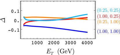
Figure 4: Variation of the jet cross section with renormalization and factorization scale. We show $\Delta$ defined in Eq. (11) versus $E_{T}$ for four choices of $\{\mu_{R}/E_{T},\mu_{F}/E_{T}\}$.

The issue of the scale dependence of the perturbative QCD calculations has received attention in the literature and various recipes have been proposed to choose ‘optimal’ values of $\mu$ (see the references in [13]). There is no compelling argument that shows that these ‘optimal’ values reduce the size of the yet unknown higher-order corrections. These recipes may thus be used to get more confidence on the central value of the theoretical calculation, but they cannot be used to reduce its theoretical uncertainty as estimated, for instance, by scale variations around $\mu\sim Q$. The theoretical uncertainty ensuing from the truncation of the perturbative series can only be reduced by actually computing more terms in perturbation theory.

We have so far discussed the factorization formula (2). We should emphasize that there is another mode of analysis of the theory available, that embodied in Monte Carlo event generator programs. In this type of analysis, one is limited (at present) to leading order partonic hard scattering cross sections. However, one simulates the complete physical process, beginning with the hard scattering and proceeding through parton showering via repeated one parton to two parton splittings and finally ending with a model for how partons turn into hadrons. This class of programs, which simulate complete events according to an approximation to QCD, are very important to the design and analysis of experiments. Current issues in Monte Carlo event generator and other related computer programs are discussed in Sect. 3

2 PARTON DISTRIBUTION FUNCTIONS

Parton distributions (pdf’s) play a central role in hard scattering cross sections at the LHC. A precise knowledge of the pdf’s is absolutely vital for reliable predictions for signal and background cross sections. In many cases, it is the uncertainty in the input pdf’s that dominates the theoretical error on the prediction. Such uncertainties can arise both from the starting distributions, obtained from a global fit to DIS, DY and other data, and from DGLAP evolution to the higher $Q^{2}$ scales typical of LHC hard scattering processes.

To predict LHC cross sections we will need accurate pdf’s over a wide range of $x$ and $Q^{2}$ (see Fig. 2). Several groups have made significant contributions to the determination of pdf’s both during and after the workshop. The MRST and CTEQ global analyses have been updated and refined, and small numerical problems have been corrected. The ‘central’ pdf sets obtained from these global fits are, not surprisingly, very similar, and remain the best way to estimate central values for LHC cross sections. Specially constructed variants of the central fits (exploring, for example, different values of $\alpha_{S}$ or different theoretical treatments of heavy quark distributions) allow the sensitivity of the cross sections to some of the input assumptions.

A rigorous and global treatment of pdf uncertainties remains elusive, but there has been significant progress in the last few years, with several groups introducing sophisticated statistical analyses into quasi-global fits. While some of the more novel methods are still at a rather preliminary stage, it is hoped that over the next few years they may be developed into useful tools.

One can reasonably expect that by LHC start-up time, the precision pdf determinations will have improved from NLO to NNLO. Although the complete NNLO splitting functions have not yet been calculated, several studies have made use of partial information (moments, $x\rightarrow 0,1$ limiting behaviour) to assess the impact of the NNLO corrections.

At the same time, accurate measurements of Standard Model (SM) cross sections at the LHC will further constrain the pdf’s. The kinematic acceptance of the LHC detectors allows a large range of $x$ and $Q^{2}$ to be probed. Furthermore, the wide variety of final states and high parton-parton luminosities available will allow an accurate determination of the gluon density and flavour decomposition of quark densities.

All of the above issues are discussed in the individual contributions that follow. Lack of space has necessarily restricted the amount of information that can be included, but more details can always be found in the literature.

2.1 MRS: pdf uncertainties and $W$ and $Z$ production at the LHC

There are several reasons why it is very difficult to derive overall ‘one sigma’ errors on parton distributions of the form $f_{i}\pm\delta f_{i}$. In the global fit there are complicated correlations between a particular pdf at different $x$ values, and between the different pdf flavours. For example, the charm distribution is correlated with the gluon distribution, the gluon distribution at low $x$ is correlated with the gluon at high $x$ via the momentum sum rule, and so on. Secondly, many of the uncertainties in the input data or fitting procedure are not ‘true’ errors in the probabilistic sense. For example, the uncertainty in the high–$x$ gluon in the MRST fits [28] derives from a subjective assessment of the impact of ‘intrinsic $k_{T}$’ on the prompt photon cross sections included in the global fit.

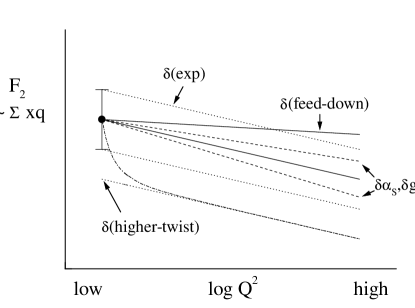
Figure 5: Schematic representation of the various uncertainties contributing to the prediction of a structure function or parton distribution at high $Q^{2}$.

Despite these difficulties, several groups have attempted to extract meaningful $\pm\delta f_{i}$ pdf errors (see [29, 30] and Sects. 2.3,2.4). Typically, these analyses focus on subsets of the available DIS and other data, which are statistically ‘clean’, i.e. free from undetermined systematic errors. As a result, various aspects of the pdf’s that are phenomenologically important, the flavour structure of the sea and the sea and gluon distributions at large $x$ for example, are either only weakly constrained or not determined at all.

Faced with the difficulties in trying to formulate global pdf errors, one can adopt a more pragmatic approach to the problem by making a detailed assessment of the pdf uncertainty for a particular cross section of interest. This involves determining which partons contribute and at which $x$ and $Q^{2}$ values, and then systematically tracing back to the data sets that constrained the distributions in the global fit. Individual pdf sets can then be constructed to reflect the uncertainty in the particular partons determined by a particular data set.

We have recently performed such an analysis for $W$ and $Z$ total cross sections at the Tevatron and LHC [10]. The theoretical technology for calculating these is very robust. The total cross sections are known to NNLO in QCD perturbation theory [31, 32, 33], and the input electroweak parameters ($M_{W,Z}$, weak couplings, etc.) are known to high accuracy. The main theoretical uncertainty therefore derives from the input pdf’s and, to a lesser extent, from $\alpha_{S}$.

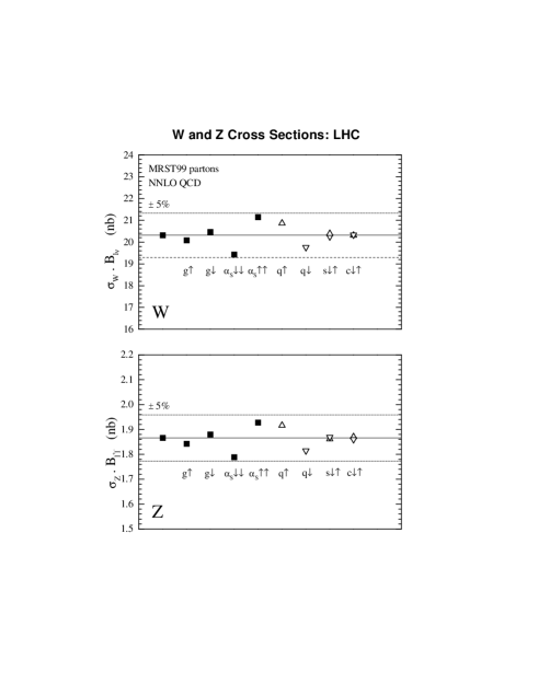
Figure 6: Predictions for the $W$ and $Z$ total cross sections times leptonic branching ratio in $pp$ collisions at $14$ TeV using the various MRST parton sets from Ref. [10]. The error bars on the default MRST prediction correspond to a scale variation of $\mu=M_{V}/2\rightarrow 2M_{V}$, $V=W,Z$.

For the hadro-production of a heavy object like a $W$ boson, with mass $M$ and rapidity $y$, leading-order kinematics give $x=M\exp(\pm y)/\sqrt{s}$ and $Q=M$. For example, a $W$ boson ($M=80$ GeV) produced at rapidity $y=3$ at the LHC corresponds to the annihilation of quarks with $x=0.00028$ and $0.11$, probed at $Q^{2}=6400$ GeV². Notice that $u,d$ quarks with these $x$ values are already more or less directly ‘measured’ in deep inelastic scattering (at HERA and in fixed–target experiments respectively), but at much lower $Q^{2}$, see Fig. 2. Therefore the first two important sources of uncertainty in the pdf’s relevant to $W$ production are

• the uncertainty in the DGLAP evolution, which except at high $x$ comes mainly from the gluon and $\alpha_{S}$;

• the uncertainty in the quark distributions from measurement errors on the structure function data used in the fit.

This is illustrated in Fig. 5. Only $75\%$ of the total $W$ cross section at the LHC arises from the scattering of $u$ and $d$ (anti)quarks. Therefore also potentially important is

• the uncertainty in the input strange ($s$) and charm ($c$) quark distributions, which are relatively poorly determined at low $Q^{2}$ scales.

In order to investigate these various effects we have constructed ten variants of the standard MRST99 distributions [10] that probe approximate $\pm 1\sigma$ variations in the gluon, $\alpha_{S}$, the overall quark normalisation, and the $s$ and $c$ pdf’s. The corresponding predictions for the $W$ total cross section at the LHC are shown in Fig. 6. Evidently the largest variation comes from the effect of varying $\alpha_{S}(M_{Z}^{2})$, in this case by $\pm 0.005$ about the central value of $0.1175$. The higher the value of $\alpha_{S}$, the faster the (upwards) evolution, and the larger the predicted $W$ cross section. The effect of a $\pm 2.5\%$ normalisation error, as parameterised by the $q\updownarrow$ pdf’s, is also significant. The uncertainties in the input $s$ and $c$ distributions get washed out by evolution to high $Q^{2}$, and turn out to be numerically unimportant.

In conclusion, we see from Fig. 6 that $\pm 5\%$ represents a conservative error on the prediction of $\sigma(W)$ at LHC. We arrive at this result without recourse to complicated statistical analyses in the global fit. It is also reassuring that the latest (corrected) CTEQ5 prediction [7] is very close to the central MRST99 prediction, see Fig. 8 below. Finally, it is important to stress that the results of our analysis represent a ‘snap-shot’ of the current situation. As further data are added to the global fit in coming years, the situation may change. However it is already clear that LHC $W$ and $Z$ cross sections can already be predicted with high precision, and their measurement will therefore provide a fundamental test of the SM.

2.2 CTEQ: studies of pdf uncertainties

Status of Standard Parton Distribution Functions

The widely used pdf sets all have been updated recently, driven mainly by new experimental inputs. Largely due to differences in the choices of these inputs (direct photon vs. jets) and their theoretical treatment, the latest MRST [10] and CTEQ [7] distributions have noticeable differences in the gluon distribution for $x>0.2$. Details are described in the original papers.

The accuracy of modern DIS measurements and the expanding $(x,Q)$ range in which pdf’s are applied require accurate QCD evolution calculations. Previously known differences in the QCD evolution codes have now been corrected; all groups now agree with established results [34] with good precision. The differences between updated pdf’s obtained with the improved evolution code and the original ones are generally small; and the differences between the physical cross sections based on the two versions of pdf’s are insignificant , by definition, since both have been fitted to the same experimental data sets. However, accurate predictions for physical processes not included in the global analysis, especially at values of $(x,Q)$ beyond the current range, can differ and require the improved pdf’s. Figs. 7a,b compare the pdf sets CTEQ5M (original) and CTEQ5M1 (updated) at scales $Q=5$ and $80$ GeV respectively.

                 

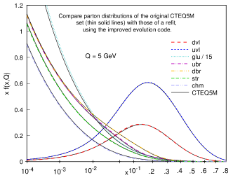
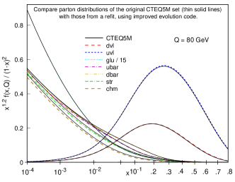
Figure 7: Comparison of CTEQ5M (original) and CTEQ5M1 (revised) distributions at two energy scales.

A comparison of the predicted $W$ production cross sections at the Tevatron and at LHC, using the historical CTEQ parton distribution sets, as well as the most recent MRST sets are given in Figs. 8. We see that the predicted values of $\sigma_{W}$ agree very well. However, the spread of $\sigma_{W}$ from different “best fit” pdf sets does not give a quantitative measure of the uncertainty of $\sigma_{W}$!

                 

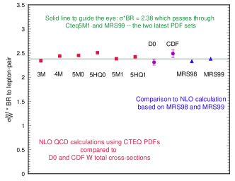
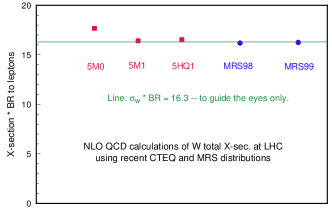
Figure 8: Predicted W production cross section, using various historical and recent parton distribution sets.

Studies of pdf Uncertainties

It is important to quantify the uncertainties of physics predictions due to imprecise knowledge of the pdf’s at future colliders (such as the LHC): these uncertainties may strongly affect the error estimates in precision SM measurements as well as the signal and backgrounds for new physics searches.

Uncertainties of the pdf’s themselves are strictly speaking unphysical, since pdf’s are not directly measurables. They are renormalization and factorization scheme dependent; and there are strong correlations between different flavours and different values of $x$ which can compensate each other in physics predictions. On the other hand, since pdf’s are universal, if one can obtain meaningful estimates of their uncertainties based on global analysis of existing data, they can then be applied to all processes that are of interest for the future.

An alternative approach is to assess the uncertainties on specific physical predictions for the full range (i.e. the ensemble) of pdf’s allowed by available experimental constraints which are used in current global analyses, without explicit reference to the uncertainties of the parton distributions themselves. This clearly gives more reliable estimates of the range of possible predictions on the physical variable under study. The disadvantage is that the results are process-specific; hence the analysis has to be carried out for each process of interest.

In this short report, we present first results from a systematic study of both approaches. In the next section we focus on the $W^{\pm}$ production cross section, as a proto-typical case of current interest. A technique of Lagrange multiplier is incorporated in the CTEQ global analysis to probe its range of uncertainty at the Tevatron and the LHC. This method is directly applicable to other cross sections of interest, e.g. Higgs production. We also plan to extend it for studying the uncertainties of $W$-mass measurements in the future. In the following section we describe a Hessian study of the uncertainties of the non-perturbative pdf parameters in general, followed by application of these to the $W^{\pm}$ production cross section study and a comparison of this result with that of the Lagrange-multiplier approach.

First, it is important to note the various sources of uncertainty in pdf analysis.

• Statistical errors of experimental data. These vary over a wide range, but are straightforward to treat.

• Systematic experimental errors within each data set typically arise from many sources, some of which are highly correlated. These errors can be treated by standard methods provided they are precisely known, which unfortunately is often not the case – either because they are not randomly distributed or their estimation may involve subjective judgements. Since strict quantitative statistical methods are based on idealized assumptions, such as random errors, one faces an important trade-off in pdf uncertainty analysis. If emphasis is put on the “rigor” of the statistical method, then most experimental data sets can not be included the analysis (see Sect. 2.3). If priority is placed on using the maximal experimental constraints from available data, then standard statistical methods need to be supplemented by physical considerations, taking into account existing experimental and theoretical limitations. We take the latter tack.

• Theoretical uncertainties arise from higher-order PQCD corrections, resummation corrections near the boundaries of phase space, power-law (higher twist) and nuclear target corrections, etc.

• Uncertainties of pdf’s due to the parametrization of the non-perturbative pdf’s, $f_{a}(x,Q^{2}_{0}),$ at some low energy scale $Q_{0}.$ The specific functional form used introduces implicit correlations between the various $x$-ranges, which could be as important, if not more so, than the experimental correlations in the determination of $f_{a}(x,Q^{2})$ for all $Q.$

In view of these considerations, the preliminary results reported here can only be regarded as the beginning of a continuing effort which will be complex, but certainly very important for the next generation of collider programs.

The Lagrange multiplier method

Our work uses the standard CTEQ5 analysis tools and results [7] as the starting point. The “best fit” is the CTEQ5M1 set. There are 15 experimental data sets, with a total of $\sim$ 1300 data points; and 18 parameters $a_{i},i=1,\dots,18$ for the non-perturbative initial parton distributions. A natural way to find the limits of a physical quantity $X$, such as $\sigma_{W}$ at $\sqrt{s}=1.8$ TeV, is to take $X$ as one of the search parameters in the global fit and study the dependence of $\chi^{2}$ for the 15 base experimental data sets on $X$.

Conceptually, we can think of the function $\chi^{2}$ that is minimized in the fit as a function of {$a_{1}$-$a_{17},X$} instead of {$a_{1}$-$a_{18}$}. This idea could be implemented directly in principle, but Lagrange’s method of undetermined multipliers does the same thing in a more efficient way. One minimizes

$$F(\lambda)=\chi^{2}+\lambda X(a_{1},\dots,a_{18})$$ (12)

for fixed $\lambda$. By minimizing $F(\lambda)$ for many values of $\lambda$, we map out $\chi^{2}$ as a function of $X$.

Figs. 9a,b show the $\chi^{2}$ for the 15 base experimental data sets as a function of $\sigma_{W}$ at the Tevatron and the LHC energies respectively. Two curves with points corresponding to specific global fits are included in each plot: one obtained with all experimental normalizations fixed; the other with these included as fitting parameters (with the appropriate experimental errors). We see that the $\chi^{2}$’s for the best fits corresponding to various values of the $W$ cross section are close to being parabolic, as expected. Indicated on the plots are 3% and 5% ranges for $\sigma_{W}$. The two curves for the Tevatron case are farther apart than for LHC, reflecting the fact that the $W$-production cross section is more sensitive to the quark/anti-quark distributions and these are tightly constrained by existing DIS data.

                 

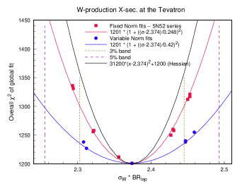
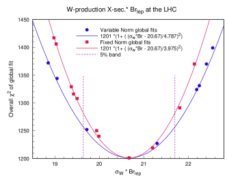
Figure 9: $\chi^{2}$ of the base experimental data sets vs. the W production cross section at the Tevatron and LHC.

The important question is: how large an increase in $\chi^{2}$ should be taken to define the likely range of uncertainty in $X$. The elementary statistical theorem that $\Delta\chi^{2}=1$ corresponds to 1 standard deviation of the measured quantity $X$ relies on assuming that the errors are Gaussian, uncorrelated, and with their magnitudes correctly estimated. Because these conditions do not hold for the full data set (of 1300 points from 15 different experiments), this theorem cannot be naively applied quantitatively. We plan to examine in some detail how well the fits along the parabolas shown in Fig.9a,b compare with the individual precision experiments included in the global analysis, in order to arrive at reasonable quantitative estimates on the uncertainty range for the $W$ cross section. In the meantime, based on past (admittedly subjective) experience with global fits, we believe a $\chi^{2}$ difference of 40-50 represents a reasonable estimate of current uncertainty of parton distributions. This implies that the uncertainty of $\sigma_{W}$ is about 3% at the Tevatron, and 5% at the LHC. These estimates certainly need to be put on a firmer basis by the on-going detailed investigation mentioned above.

The Hessian matrix method

The Hessian matrix is a standard procedure for error analysis. At the minimum of $\chi^{2}$, the first derivatives with respect to the parameters $a_{i}$ are zero, so near the minimum $\chi^{2}$ can be approximated by

$$\chi^{2}=\chi^{2}_{0}+\frac{1}{2}\sum_{i,j}F_{ij}y_{i}y_{j}$$ (13)

where $y_{i}=a_{i}-a_{0i}$ is the displacement from the minimum, and $F_{ij}$ is the Hessian, the matrix of second derivatives. It is natural to define a new set of coordinates using the complete orthonormal set of eigenvectors of the symmetric matrix $F_{ij}$. These vectors can be ordered by their eigenvalues $e_{i}$. The eigenvalues indicate the uncertainties for displacements along the eigenvectors. For uncorrelated Gaussian statistics, the quantity $\ell_{i}=1/\sqrt{e_{i}}$ is the distance in the 18 dimensional parameter space that gives a unit increase in $\chi^{2}$ in the direction of eigenvector $i$.

From calculations of the Hessian we find the eigenvalues vary over a wide range. There are “steep” directions of $\chi^{2}$ – combinations of parameters that are well determined – e.g. parameters for $u$ and $d$, which are well-constrained by DIS data. There are also “flat” directions where $\chi^{2}$ changes little over large distance in $a_{i}$ space, some of them associated with the gluon distribution. These flat directions are inevitable in global fitting, because as the data improve it makes sense to maintain enough flexibility for $f_{a}(x,Q^{2}_{0})$ to be determined by the available experimental constraints. The Hessian method gives an analytic picture of the region in parameter space around the minimum, hence allows us to identify the particular degrees of freedom which need further experimental input in future global analyses.

We have calculated how the $W$ cross section $\sigma_{W}$ varies along the eigenvectors of the Hessian. Details will be described elsewhere. This provides another way to calculate the relation between the minimum $\chi^{2}$ for the base experimental data sets and the value of $\sigma_{W}$. The results are shown as the third line in Fig. 9a. We see that there is approximate agreement between this method and the Lagrange multiplier method. Armed with the Hessian, one can in principle make similar calculations on other physical cross sections without having to do repeated global fits as in the Lagrange multiplier method. The latter, however, gives more reliable bounds for each individual process.

Conclusion

We have just begun the task of determining quantitative uncertainties for the parton distribution functions and their physics predictions. The methods developed so far look promising. Related work reported in this Workshop (see [10, 35, 36, 37] and Sects. 2.1,2.3,2.4) share the same objectives, but have rather different emphases, some of which are briefly mentioned in the text. These complementary approaches should lead to eventual progress which is critical for the high-energy physics program at LHC, as well as at other colliders.

2.3 Pdf uncertainties

Introduction

The goal of our work is to extract pdf’s from data with a quantitative estimation of the uncertainties. There are some qualitative tools that exist to estimate the uncertainties, see e.g. [28]. These tools are clearly not adequate when the pdf uncertainties become important. One crucial example of a measurement that will need a quantitative assessment of the pdf uncertainty is the planned high precision measurement of the mass of the $W$-vector boson at the Tevatron.

The method we have developed in [35] is flexible and can accommodate non-Gaussian distributions for the uncertainties associated with the data and the fitted parameters as well as all their correlations. New data can be added in the fit without having to redo the whole fit. Experimenters can therefore include their own data into the fit during the analysis phase, as long as correlation with older data can be neglected. Within this method it is trivial to propagate the pdf uncertainties to new observables, there is for example no need to calculate the derivative of the observable with respect to the different pdf parameters. The method also provides tools to assess the goodness of the fit and the compatibility of new data with current fit. The computer code has to be fast as there is a large number of choices in the inputs that need to be tested.

It is clear that some of the uncertainties are difficult to quantify and it might not be possible to quantify all of them. All the plots presented here are for illustration of the method only, our results are preliminary. At the moment we are not including all the sources of uncertainties and our results should therefore be considered as lower limits on the pdf uncertainties. Note that all the techniques we use are standard, in the sense that they can be found in books and papers on statistics [38, 39] and/or in Numerical Recipes.

Outline of the Method

We only give a brief overview of the method in this section. More details are available in [35]. Once a set of core experiments is selected, a large number of uniformly distributed sets of parameters $\lambda\equiv\lambda_{1},\lambda_{2},\ldots,\lambda_{N_{par}}$ (each set corresponds to one pdf) can be generated. The probability of each set, $P(\lambda)$, can be calculated from the likelihood (the probability) that the predictions based on $\lambda$ describe the data, assuming that the initial probability distribution of the parameters is uniform, see [38, 39].

Knowing $P(\lambda)$, the probability of the possible values of any observable (quantity that depends on $\lambda$) can be calculated using a Monte Carlo integration. For example, the average value and the pdf uncertainty of an observable $x$ are given by:

$$\mu_{x}=\int\left(\prod_{i=1}^{N_{par}}d\lambda_{i}\right)\,x(\lambda)P(\lambda),\qquad\sigma_{x}^{2}=\int\left(\prod_{i=1}^{N_{par}}d\lambda_{i}\right)\,(x(\lambda)-\mu_{x})^{2}P(\lambda)$$

Note that the average value and the standard deviation represents the distribution only if the latter is a Gaussian. The above is correct but computationally inefficient, instead we use a Metropolis algorithm to generate $N_{pdf}$ unweighted pdf’s distributed according to $P(\lambda)$. Then:

$$\mu_{x}\approx\frac{1}{N_{pdf}}\sum_{j=1}^{N_{pdf}}x\left(\lambda_{j}\right),\qquad\qquad\sigma_{x}^{2}\approx\frac{1}{N_{pdf}}\sum_{j=1}^{N_{pdf}}\left(x\left(\lambda_{j}\right)-\mu_{x}\right)^{2}\ .$$

This is equivalent to importance sampling in Monte Carlo integration techniques and is very efficient. Given the unweighted set of pdf’s, a new experiment can be added to the fit by assigning a weight (a new probability) to each of the pdf’s, using Bayes’ theorem. The above summations become weighted. There is no need to redo the whole fit if there is no correlation between the old and new data. If we know how to calculate $P(\lambda)$ properly, the only uncertainty in the method comes from the Monte-Carlo integrations.

Calculation of $P(\lambda)$

Given a set of experimental points $\{x^{e}\}=x^{e}_{1},x^{e}_{2},\ldots,x^{e}_{N_{obs}}$ the probability of a set of pdf is proportional to the likelihood, the probability of the data given that the theory is derived from that set of pdf: $P(\lambda)\approx P(\{x^{e}\}|\lambda)$. If all the uncertainties are Gaussian distributed, then it is well known that: $P({x^{e}}|\lambda)\approx e^{-\frac{\chi^{2}}{2}}$, where $\chi^{2}$ is the usual chi-square. It is only in this case that it is sufficient to report the size of the uncertainties and their correlation. When the uncertainties are not Gaussian distributed, it is necessary for experiments to report the distribution of their uncertainties and the relation between these uncertainties the theory and the value of the measurements. Unfortunately most of the time that information is not reported, or difficult to extract from papers. This is a very important issue that has been one of the focus of the pdf working group at a Fermilab workshop in preparation for run II [40]. In other words, experiments should always provide a way to calculate the likelihood of their data given a theory prediction for each of their measured data point ($P(\{x^{e}\}|\lambda)$). This was also the unanimous conclusion of a recent workshop on confidence limits held at CERN [41]. This is particularly crucial when combining different experiments together: the pull of each experiment will depend on it and, as a result, so will the central values of the deduced pdf’s. Another problem that is sometimes underestimated is the fact that some if not all systematic uncertainties are in fact proportional to the theory. Ignoring this fact while fitting for the parameters can lead to serious bias.

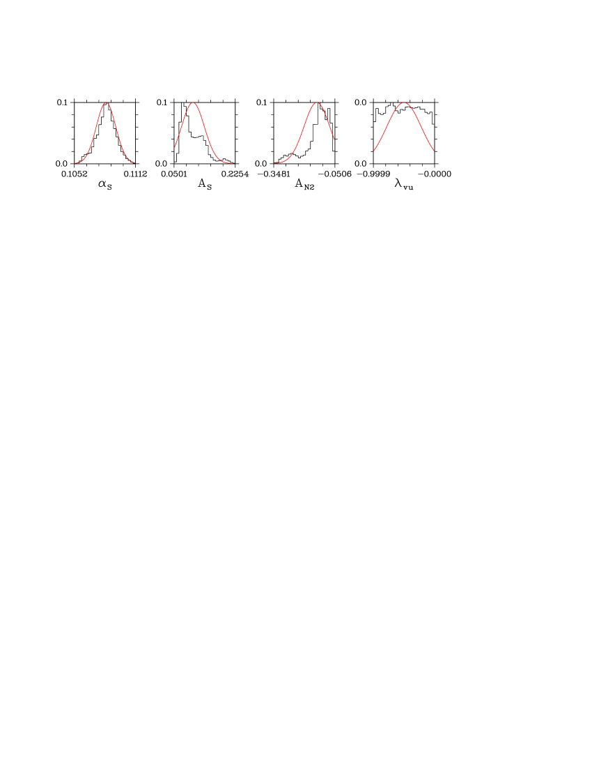
Figure 10: Plot of the distribution (histogram) of four of the parameters. The first one is $\alpha_{\mathrm{S}}$, the strong coupling constant at the mass of the $Z$-boson. The line is a Gaussian distribution with same average and standard deviation as the histogram.

Sources of uncertainties

There are many sources of uncertainties beside the experimental uncertainties. They either have to be shown to be small enough to be neglected or they need to be included in the pdf uncertainties. For examples: variation of the renormalization and factorization scales; non-perturbative and nuclear binding effects; the choice of functional form of the input pdf at the initial scale; accuracy of the evolution; Monte-Carlo uncertainties; and the theory cut-off dependences.

Current fit

Draconian measures were needed to restart from scratch and re-evaluate each issue. We fixed the renormalization and factorisation scales, avoided data affected by nuclear binding and non-perturbative effects, and use a MRS-style parametrization for the input pdf’s. The evolution of the pdf is done by Mellin transform method, see [42, 43]. All the quarks are considered massless. We imposed a positivity constraint on $F_{2}$. A positivity constraint on other “observables” could also be imposed.

At the moment we are using H1 and BCDMS(proton) measurement of $F_{2}^{p}$ for our core set. The full correlation matrix is taken into account. Assuming that all the uncertainties are Gaussian distributed  we calculate the $\chi^{2}(\lambda)$ and $P(\lambda)\approx exp(-\chi^{2}/2)$. We generated 50000 unweighted pdf’s according to the probability function. For 532 data points, we obtained a minimum $\chi^{2}=530$ for 24 parameters. We have plotted in Fig. 10, the probability distribution of some of the parameters. Note that the first parameter is $\alpha_{\mathrm{S}}$. The value is smaller than the current world average. However, it is known that the experiments we are using prefer a lower value of this parameter, see [44], and as already pointed out, our current uncertainties are lower limits. Note that the distribution of the parameter is not Gaussian, indicating that the asymptotic region is not reached yet. In this case, the blind use of a so-called chi-squared fitting technique is not appropriate. From this large set of pdf’s, it is straightforward to plot, for example, the correlation between different parameters and to propagate the uncertainties to other observables.

2.4 Uncertainties on pdf’s and parton-parton luminosities

Figure 11: The relative uncertainties for selected set of parton luminosities (full lines: experimental errors (stat+syst); short-dashed lines: RS; dotted-dashed lines: TS; sparse-dotted lines: DC; dense-dotted lines: MC; long-dashed lines: SS). Here $L_{\rm GG}$ is gluon-gluon luminosity; $L_{\rm qq}=L_{\rm uu}+L_{\rm dd}+L_{\rm du}$; $L_{\rm q\bar{q}}=L_{\rm u\bar{d}}+L_{\rm d\bar{u}}$; $L_{\rm(q+\bar{q})G}=L_{\rm uG}+L_{\rm\bar{u}G}+L_{\rm dG}+L_{\rm\bar{d}G}$.

An important quantity for LHC physics is the uncertainty of pdf’s used for the cross section calculations. The modern widely used pdf’s parametrizations do not contain complete estimate of their uncertainties. This estimate is difficult partially due to the lack of experimental information on the data points correlations, partially due to the fact that the theoretical uncertainties are conventional, and partially due to the fundamental problem of restoring the distribution from the finite number of measurements. These problems are not completely solved at the moment and a comprehensive estimate of the pdf’s uncertainties is not available so far. The study given below is based on the NLO QCD analysis of the world charged leptons DIS data of Refs. [45, 46, 47, 48, 49, 50, 51] for proton and deuterium targets. The analysed data span the region $x=10^{-4}\div 0.75$, $Q^{2}=2.5\div 5000$ GeV², $W\mathrel{\hbox to0.0pt{\lower 4.0pt\hbox{\hskip 1.0pt$\sim$}\hss}\raise 1.0pt\hbox{$>$}}2$ GeV and allows for precise determination of pdf’s at low $x$, which is important for LHC since the most of accessible processes are related to small $x$. The data are accompanied by the information on point-to-point correlations due to systematic errors. This allows the complete inference of systematic errors, that was performed using the covariance matrix approach, as in Ref. [36]. The pdf’s uncertainties due to the variation of the strong coupling constant $\alpha_{\mathrm{S}}$ and the high twists (HT) contribution are automatically accounted for in the total experimental uncertainties since $\alpha_{\mathrm{S}}$ and HT are fitted. Other theoretical errors on pdf’s were estimated as the pdf’s variation after the change of different fit ansatzes:

• – the change of renormalization scale in the evolution equations from $Q^{2}$ to $4Q^{2}$. This uncertainty is evidently connected with the influence of NNLO corrections.

• – the change of threshold value of $Q^{2}$ for the QCD evolution loops with heavy quarks from $m_{\rm Q}^{2}$ to $6.5m_{\rm Q}^{2}$. The variation is conventional and was chosen following the arguments of Ref. [52].

• – the change of correction on nuclear effects in deuterium from the ansatz based on the Fermi motion model of Ref. [53] to the phenomenological formula from Ref. [54]. Note that this uncertainty may be overestimated in view of discussions [55, 56] on the applicability of the model of Ref.[54] to light nuclei.

• – the change of c-quark mass by 0.25 GeV (the central value is 1.5 GeV).

• – the change of strange sea suppression factor by 0.1, in accordance with recent results by the NuTeV collaboration [57] (the central value is 0.42).

One can see that the scale of the theoretical errors is conventional and can change with improvements in the determination of the fit input parameters and progress in theory. Moreover, the uncertainties can be correlated with the uncertainties of the partonic cross sections, e.g. the effect of RS uncertainty on pdf’s can be compensated by the NNLO correction to parton cross section. Thus the theoretical uncertainties should not be applied automatically to any cross section calculations, contrary to experimental ones.

Figure 12: The ratios of the experimental pdf’s errors calculated with some fitted parameters fixed to the pdf’s errors calculated with all parameters released ($\alpha_{\mathrm{S}}$ fixed – a); HT fixed – b)). The similar ratio for the systematic errors omitted/included is also given – c). Full lines correspond to gluons, dashed ones – to total sea, dotted ones – to d-quarks, dashed-dotted ones – to u-quarks.

The pdf’s uncertainties have different importance for various processes. The limited space does not allow us to review all of them. We give the figures for the most generic ones only. The uncertainties of a specific cross section due to pdf’s are entirely located in the uncertainties of the parton-parton luminosity $L_{ab}$, that is defined as

$$L_{ab}(M)=\frac{1}{s}\int^{1}_{\tau}\frac{dx}{x}\;f_{a}(x,M^{2})f_{b}(\tau/x,M^{2}),$$

where $M$ is the produced mass and $\tau=M^{2}/s$. In Fig. 11 the uncertainties for selected set of parton luminosities calculated using the pdf’s from Ref. [29] are given. The upper bound of $M$ was chosen so that the corresponding luminosity is $\sim 0.01$ pb. One can see that in general at $M\mathrel{\hbox to0.0pt{\lower 4.0pt\hbox{\hskip 1.0pt$\sim$}\hss}\raise 1.0pt\hbox{$>$}}1$ TeV experimental uncertainties dominate, while at $M\mathrel{\hbox to0.0pt{\lower 4.0pt\hbox{\hskip 1.0pt$\sim$}\hss}\raise 1.0pt\hbox{$<$}}1$ TeV theoretical ones dominate. Of the latter the most important are the RS uncertainty for the gluon luminosity and MC uncertainty for the quark luminosities. At the largest $M$ the DC uncertainty for quark-quark luminosity is comparable with the experimental one. In the whole the uncertainties do not exceed 10% at $M\mathrel{\hbox to0.0pt{\lower 4.0pt\hbox{\hskip 1.0pt$\sim$}\hss}\raise 1.0pt\hbox{$<$}}1$ TeV. As for the quark-quark luminosity, its uncertainty is less than 10% in the whole $M$ range. The uncertainties are not so large in view of the fact that only a small subset of data relevant for the pdf’s extraction was used in the analysis. Adding data on prompt photon production, DY process, and jet production can improve the pdf’s determination at large $x$. Meanwhile it is worth to note that high order QCD corrections are more important for these processes than for DIS and the decrease of experimental errors due to adding data points can be accompanied by the increase of theoretical errors.

Figure 13: The pdf’s correlation coefficients.

As it was noted above, the experimental pdf’s errors by definition include the statistical and systematical errors, as well as errors due to $\alpha_{\mathrm{S}}$ and HT. To trace the effect of $\alpha_{\mathrm{S}}$ variation on the pdf’s uncertainties the latter were re-calculated with $\alpha_{\mathrm{S}}$ fixed at the value obtained in the fit. The ratios of obtained experimental pdf’s errors to the errors calculated with $\alpha_{\mathrm{S}}$ released are given in Fig. 12. It is seen that the $\alpha_{\mathrm{S}}$ variation takes some effect on the gluon distribution errors only. Similar ratios for the HT fixed are also given in Fig. 12. One can conclude, that the account of HT contribution have significant impact on the pdf’s errors. Meanwhile it is evident that these ratios hardly depend on the scale of pdf’s error and are specific for the analysed data set. For instance, in the analysis of CCFR data on the structure function $F_{3}$ no significant influence of HT on the pdf’s was observed [58, 59]. The contribution of systematic errors to the total experimental pdf’s uncertainties is also given in Fig. 12: the systematic errors are most essential for the u- and d-quark distributions.

	stat+syst	RS	TS	SS	MC	DC
$\Delta L_{\rm W}(\%)$	1.9	0.4	0.9	1.3	2.9	0.3
$\Delta L_{\rm Z}(\%)$	1.6	0.5	0.9	1.3	2.9	0.6
$\Delta L_{\rm W/Z}(\%)$	0.5	–	–	–	–	0.3

Table 1: The uncertainties of the parton luminosities for $W/Z$ production cross sections and their ratios. Here $L_{\rm W}=L_{\rm u\bar{d}}+L_{\rm d\bar{u}}$, $L_{\rm Z}=L_{\rm u\bar{u}}+L_{\rm d\bar{d}}$, and $L_{\rm W/Z}=(L_{\rm u\bar{d}}+L_{\rm d\bar{u}})/(L_{\rm u\bar{u}}+L_{\rm d\bar{d}})$.

Except uncertainties itself the pdf correlation are also important (see Fig. 13). The account of correlations can lead to cancellation of the pdf’s uncertainties in the calculated cross section. The luminosities uncertainties can also cancel in the ratios of cross sections. An example of such cancellation is given in Table 1, where the uncertainties of luminosities for the $W/Z$ production cross sections and their ratios are given.

The pdf set discussed in this subsection can be obtained by the code [60]. The pdf’s are DGLAP evolved in the range $x=10^{-7}\div 1$, $Q^{2}=2.5\div 5.6\cdot 10^{7}$ GeV². The code returns the values of u-, d-, s-quark, and gluon distributions Gaussian-randomized with accordance of their dispersions and correlations including both experimental and theoretical ones.

2.5 Approximate NNLO evolution of parton densities

In order to arrive at precise predictions of perturbative QCD for the LHC, for example for the total $W$-production cross section discussed in Sects. 2.1 and 2.2, the calculations need to be extended beyond the NLO. Indeed, the NNLO coefficient functions for the above cross section have been calculated some time ago [32, 33]. The same holds for the structure functions in DIS [61, 62, 63, 64] which form the backbone of the present information on the parton densities. On the other hand, the corresponding NNLO splitting functions have not been computed so far. Partial results are however available, notably the lowest four and five even-integer moments, respectively, for the singlet and non-singlet combinations [25, 26]. When supplemented by results on the leading $x\!\rightarrow\!0$ terms [65, 66, 67, 68, 69] derived from small-$x$ resummations, these constraints facilitate effective parametrisations [70, 71] which are sufficiently accurate for a wide range in $x$ (and thus a wide range of final-state masses at the LHC). In this section, we compile these expressions and take a brief look at their implications. For detailed discussions the reader is referred to refs. [70, 71].

In terms of the flavour non-singlet (NS) and singlet (S) combinations of the parton densities (here $f_{q_{f}}\equiv q$ and $f_{g}\equiv g$),

$$q_{{\rm NS},ik}^{\pm} \!=\! q_{i}\pm\bar{q}_{i}-(q_{k}\pm\bar{q}_{k})\>\>,\quad\quad q_{\rm NS}^{V}\,=\,\sum_{r=1}^{N_{f}}(q_{r}-\bar{q}_{r})\>,\quad\quad q_{\rm S}^{\,}\,=\,\left(\begin{array}[]{c}\!\Sigma\!\\ \!g\!\end{array}\right)$$ (16)

with $\Sigma=\sum_{r=1}^{N_{f}}(q_{r}+\bar{q}_{r})$, the evolution equations (8) consist of $\,2N_{f}\!-\!1\,$ scalar non-singlet equations and the $2\!\times\!2$ singlet system. The LO and NLO splitting functions $P^{(LO)}(x)$ and $P^{(NLO)}(x)$ in Eq. (9) are known for a long time. For each of the NNLO functions $P^{(2)}(x)=(4\pi)^{3}P^{(NNLO)}(x)$ two approximate expressions (denoted by ‘$A$’ and ‘$B$’) are given below in the $\overline{\mbox{MS}}$ scheme, which span the estimated residual uncertainty. The central results are represented by the average $1/2\,(P_{A}^{(2)}+P_{B}^{(2)})$.

The NS⁺ parametrisations [70] read, using $\,\delta\equiv\delta(1\!-\!x)$, $\,L_{1}\equiv\ln(1\!-\!x)$ and $\,L_{0}\equiv\ln x$,

$$P^{(2)+}_{{\rm NS},A}(x)=\frac{1137.897}{(1-x)_{+}}+1099.754\,\delta-2975.371\,x^{2}-125.243-64.105\,L_{0}^{2}+1.580\,L_{0}^{4}$$

$$\mbox{}-N_{f}\left(\frac{184.4098}{(1-x)_{+}}+180.6971\,\delta+98.5885\,L_{1}-205.7690\,x^{2}-6.1618-5.0439\,L_{0}^{2}\right)+P^{(2)}_{{\rm NS},N_{f}^{2}}\>\>,$$

$$P^{(2)+}_{{\rm NS},B}(x)=\frac{1347.207}{(1-x)_{+}}+2283.011\,\delta-722.137\,L_{1}^{2}-1236.264-332.254\,L_{0}+1.580\,(L_{0}^{4}-4L_{0}^{3})$$

$$\mbox{}-N_{f}\left(\frac{184.4098}{(1-x)_{+}}+180.6971\,\delta+98.5885\,L_{1}-205.7690\,x^{2}-6.1618-5.0439\,L_{0}^{2}\right)+P^{(2)}_{{\rm NS},N_{f}^{2}}$$

with

$$P^{(2)}_{{\rm NS},N_{f}^{2}}(x)\> = \frac{1}{81}\bigg{(}\mbox{}-\frac{64}{(1-x)_{+}}-[204+192\,\zeta(3)-320\,\zeta(2)]\,\delta(1-x)+64$$ (18)

$$\mbox{}+\frac{x\ln x}{1-x}\,(96\,\ln x+320)+(1-x)(48\,\ln^{2}x+352\ln x+384)\bigg{)}\>\>.$$

Here $\zeta(l)$ denotes Riemann’s $\zeta$-function. Equation (18) is an exact result, derived from large-$N_{f}$ methods [72]. The corresponding expressions for $P^{(2)-}_{{\rm NS}}$ are

$$P^{(2)-}_{{\rm NS},A}(x) \!=\! P^{(2)+}_{{\rm NS},A}(x)+20.687\,x^{2}-18.466+66.866\,L_{0}^{2}-0.148\,L_{0}^{4}$$ (19)

$$\mbox{}+N_{f}\left(0.0163\,L_{1}-0.402\,x^{2}+0.4122\,-1.4965L_{0}^{2}\right)\>\>,$$

$$P^{(2)-}_{{\rm NS},B}(x) \!=\! P^{(2)+}_{{\rm NS},B}(x)-0.101\,L_{1}^{2}+1.508+4.775\,L_{0}-0.148\,(L_{0}^{4}-4L_{0}^{3})$$

$$\mbox{}+N_{f}\left(0.0163\,L_{1}-0.402\,x^{2}+0.4122\,-1.4965L_{0}^{2}\right)\>\>.$$

The difference between $P^{(2)-}_{\rm NS}$ and $P^{(2)V}_{\rm NS}$ is unknown, but expected to have a negligible effect ($\ll 1\%$).

The effective parametrisations for the singlet sector are given in Ref. [71]. Besides the $1/x\,\ln x$ terms of $P_{qq}^{(2)}$, $P_{qg}^{(2)}$ and $P_{gg}^{(2)}$ [66, 67], only the $N_{f}^{2}$ contribution $\propto 1/[1-x]_{+}$ to $P_{gg}^{(2)}$ is exactly known here [73].

The evolution equations (8) are written for a factorization scale $\mu_{f}=Q$. Their form can be straightforwardly generalized to include also the dependence on the renormalization scale $\mu_{r}$.

The expansion of Eq. (8) is illustrated in the left part of Fig. 14 for $\,\mu_{r}\!=\!\mu_{f}$, $\,\alpha_{\mathrm{S}}\!=\!0.2$ and parton densities typical for $\,\mu_{f}^{2}\simeq 30\mbox{ GeV}^{2}$. Under these conditions, the NNLO effects are small ($<\!2\%$) at medium and large $x$. This also holds for the non-singlet evolution not shown in the figure. The approximate character of the our results for $P^{(2)}$ does not introduce relevant uncertainties at $x\mathrel{\hbox to0.0pt{\lower 4.0pt\hbox{\hskip 1.0pt$\sim$}\hss}\raise 1.0pt\hbox{$>$}}2\cdot 10^{-3}$. The third-order corrections increase with decreasing $x$, reaching $(12\pm 4)\%$ and $(\mbox{}-6\pm 3)\%$, respectively, of the NLO predictions for $\dot{\Sigma}$ and $\dot{g}$ at $x=10^{-4}$.

The renormalization-scale uncertainty of these results is shown in the right part of Fig. 14 in terms of $\Delta_{\mu_{r}}\dot{q}\equiv(\dot{q}_{\rm max}-\dot{q}_{\rm min})/[2\,\dot{q}_{\rm average}]$, as determined over the range $0.5\,\mu_{f}\leq\mu_{r}\leq 2\,\mu_{f}$. Note that the spikes slightly below $x=0.1$ arise from $\dot{q}_{\rm average}\simeq 0$ and do not represent enhanced uncertainties. Thus the inclusion of the third-order terms in Eq. (8), already in its approximate form, leads to significant improvements of the scale stability, except for the gluon evolution below $x=10^{-3}$.

Figure 14: Left: The LO, NLO and approximate NNLO predictions for the logarithmic derivatives $\dot{q}/q\equiv d\ln q/d\ln\mu_{f}^{2}$ of the singlet quark and gluon densities, $q=\Sigma$ and $q=g$, at $\mu_{f}^{2}\simeq 30\mbox{ GeV}^{2}$. Right: The relative scale uncertainty $\Delta_{\mu_{r}}\dot{q}$ (defined in the text) of these NLO and NNLO results. The number of flavours is $N_{f}=4$.

2.6 The NNLO analysis of the experimental data for $xF_{3}$ and the effects of high-twist power corrections

During the last few years there has been considerable progress in calculations of the perturbative QCD corrections to characteristics of DIS. Indeed, the analytic expressions for the NNLO perturbative QCD corrections to the coefficient functions of structure functions $F_{2}$ [61, 62, 64] and $xF_{3}$ [63, 74] are now known. However, to perform the NNLO QCD fits of the concrete experimental data it is also necessary to know the NNLO expressions for the anomalous dimensions of the moments of $F_{2}$ and $xF_{3}$. At present, this information is available in the case of $n=2,4,6,8,10$ moments of $F_{2}$ [25, 26]. The results of Refs. [61, 62, 63, 64, 25, 26, 74] are forming the theoretical background for the study of the effects, contributing to scaling violation at the level of new theoretical precision, namely with taking into account the effects of the NNLO perturbative QCD contributions.

In the process of these studies it is rather instructive to include the available theoretical information on the effects of high-twist corrections, which could give rise to scaling violation of the form $1/Q^{2}$. The development of the infrared renormalon (IRR) approach (for a review see Ref. [75]) and the dispersive method [76] (see also [77, 78]) made it possible to construct models for the power-suppressed corrections to DIS structure functions (SFs). Therefore, it became possible to include the predictions of these models to the concrete analysis of the experimental data.

In this part of the Report the results of the series of works [58, 59, 79, 80] will be summarized. These works are devoted to the analysis of the experimental data of $xF_{3}$ SF of $\nu N$ DIS, obtained by the CCFR collaboration [81]. They have the aim to determine the NNLO values of $\Lambda_{\overline{MS}}^{(4)}$ and $\alpha_{\mathrm{S}}(M_{Z})$ with fixation of theoretical ambiguities due to uncalculated higher-order perturbative QCD terms and transitions from the case of $f=4$ number of active flavours to the case of $f=5$ number of active flavours. The second task was to extract the effects of the twist-4 contributions to $xF_{3}$ [58, 80] and compare them with the IRR-model predictions of Ref. [82]. Some estimates of the influence of the twist-4 corrections to the constants of the initial parametrization of $xF_{3}$ [59] are presented. These constants are related to the parton distribution parameters.

The analysis of Refs. [58, 59, 79, 80] is based on reconstruction of the non-singlet (NS) SF $xF_{3}$ from the finite number of its moments $M_{n}(Q^{2})=\int_{0}^{1}x^{n-1}F_{3}(x,Q^{2})dx$ using the Jacobi polynomial method, proposed in Ref. [83] and further developed in Refs. [84, 85, 86, 87]. Within this method one has

$$xF_{3}(x,Q^{2})=x^{\alpha}(1-x)^{\beta}\sum_{n=0}^{N_{max}}\Theta_{n}^{\alpha,\beta}(x)\sum_{j=0}^{n}c_{j}^{(n)}(\alpha,\beta)M_{j+2}^{TMC}(Q^{2})$$ (20)

where $\Theta_{n}^{\alpha,\beta}$ are the Jacobi polynomials, $c_{j}^{(n)}(\alpha,\beta)$ are combinatorial coefficients given in terms of Euler $\Gamma$-functions and the $\alpha$, $\beta$-weight parameters. In view of the reasons, discussed in Ref. [58] they were fixed to 0.7 and 3 respectively, while $N_{max}=6$ was taken. Note, that the expressions for Mellin moments were corrected by target mass contributions (TMC), taken into account as $M_{n}^{TMC}(Q^{2})=M_{n}(Q^{2})+(n(n+1)/(n+2))(M_{nucl}^{2}/Q^{2})M_{n+2}(Q^{2})$. The QCD evolution of the moments is defined by the solution of the corresponding renormalization group equation

$$\frac{M_{n}(Q^{2})}{M_{n}(Q_{0}^{2})}=exp\bigg{[}-\int_{A_{s}(Q_{0}^{2})}^{A_{s}(Q^{2})}\frac{\gamma_{NS}^{(n)}(x)}{\beta(x)}dx\bigg{]}\frac{C_{NS}^{(n)}(A_{s}(Q^{2}))}{C_{NS}^{(n)}(A_{s}(Q_{0}^{2}))}$$ (21)

The QCD running coupling constant enters this equation through $A_{s}(Q^{2})=\alpha_{\mathrm{S}}(Q^{2})/(4\pi)$ and is defined as the expansion in terms of inverse powers of $ln(Q^{2}/\Lambda_{\overline{MS}}^{(4)~{}2})$-terms in the LO, NLO and NNLO. The NNLO approximation of the coefficient functions of the moments $C_{NS}^{(n)}(A_{s}(Q^{2}))=1+C^{(1)}(n)A_{s}(Q^{2})+C^{(2)}(n)A_{s}^{2}(Q^{2})$ were determined from the results of Ref. [63, 74]. The related anomalous dimension functions are defined as

$$\mu\frac{\partial lnZ_{n}^{NS}}{\partial\mu}=\gamma_{NS}^{(n)}(A_{s})=\sum_{i\geq 0}\gamma_{NS}^{(i)}(n)A_{s}^{i+1}$$ (22)

where $Z_{n}^{NS}$ are the renormalization constants of the corresponding NS operators. The expression for the QCD $\beta$-function in the $\overline{MS}$-scheme is known analytically at the NNLO [11, 88]. However, as was already mentioned, the NNLO corrections to $\gamma_{NS}^{(n)}$ are known at present only in the case of $n=2,4,6,8,10$ NS moments of $F_{2}$ SF of $eN$ DIS [25, 26]. Keeping in mind that in these cases the difference between the NLO expressions for $\gamma_{NS,F_{2}}^{(1)}$ and $\gamma_{NS,xF_{3}}^{(1)}$ is rather small [79], it was assumed that the similar feature is true at the NNLO also. The $xF_{3}$ fits of Refs. [58, 59, 79, 80] were done within this approximation. The one more approximation, entering onto these analysis, was the estimation of the anomalous dimensions of odd moments with $n=3,5,7,9$ by means of smooth interpolation of the results of Refs. [25, 26], originally proposed in Ref. [89]. In view of the basic role of the NNLO corrections to the coefficient functions of $xF_{3}$ moments, revealed in the process of the concrete fits [58, 59, 79, 80], it is expected that neither the calculations of the NNLO corrections to $xF_{3}$ odd anomalous dimensions (which are now in progress [90]) and further interpolation to even values of $n$, nor the fine-tuning of the reconstruction method of Eq. (20), which depends on the values of $\alpha$, $\beta$ and $N_{max}$, will not affect significantly the accuracy of the main results of Refs. [58, 59, 80].

The power corrections were included in the analysis using two different approaches. First, following the ideas of Ref. [91], the term $h(x)/Q^{2}$ was added onto the r.h.s. of Eq. (20). The function $h(x)$ was parameterized by a set of free constants $h_{i}$ for each $x$-bin of the analysed data. These constants were extracted from the concrete LO, NLO and NNLO fits. The resulting behaviour of $h(x)$ is presented in Fig. 15, taken from Ref. [58]. Secondly, the IRR model contribution $M_{n}^{IRR}=\tilde{C}(n)M_{n}(Q^{2})A_{2}^{{}^{\prime}}/Q^{2}$ was added into the reconstruction formula of Eq. (20), where $A_{2}^{{}^{\prime}}$ is the free parameter and was estimated in Ref. [82]. The factor $M_{n}(Q_{0}^{2})$ in the l.h.s. of Eq. (21) was defined at the initial scale $Q_{0}^{2}$ using the parametrization $xF_{3}(x,Q_{0}^{2})=A(Q_{0}^{2})x^{b(Q_{0}^{2})}(1-x)^{c(Q_{0}^{2})}(1+\gamma(Q_{0}^{2})x)$. In Table 2 the combined results of the fits of Refs. [58, 59] of CCFR’97 data are presented. The twist-4 terms were switched off and retained following the discussions presented above.

The comments on the extracted behaviour of $h(x)$ (see Fig. 15) are now in order. Its $x$-shape, obtained from LO and NLO analysis of Ref. [58] is in agreement with the IRR-model formula of Ref. [82]. Note also, that the combination of quark counting rules [92, 93] with the results of Ref. [94, 95] predict the following $x$-shape of $h(x)$: $h(x)\sim A_{2}^{{}^{\prime}}(1-x)^{2}$. Taking into account the negative values of $A_{2}^{{}^{\prime}}$, obtained in the process of LO and NLO fits (see Table 2), one can conclude, that the related behaviour of $h(x)$ is in qualitative agreement with these predictions. Though a certain indication of the twist-4 terms survives even at the NNLO, the NNLO part of Fig. 15 demonstrates that the $x$-shape of $h(x)$ starts to deviate from the IRR model of Ref. [82]. Notice also, that within the statistical error bars the NNLO value of $A_{2}^{{}^{\prime}}$ is indistinguishable from zero (see Table 2). This feature might be related to the interplay between NNLO perturbative and $1/Q^{2}$ corrections. Moreover, at the used reference scale $Q_{0}^{2}=20~{}GeV^{2}$ the high-twist parameters cannot be defined independently from the effects of perturbation theory, which at the NNLO can mimic the contributions of higher-twists provided the experimental data is not precise enough and the value of $Q_{0}^{2}$ is not too small (for the recent discussion of this subject see Refs. [29, 30]).

Order	$\Lambda_{\overline{MS}}^{(4)}$	A	b	c	$\gamma$	$A_{2}^{{}^{\prime}}$[$GeV^{2}$]	$\chi^{2}$/points
LO	264$\pm$ 36	4.98$\pm$ 0.23	0.68$\pm$ 0.02	4.05$\pm$ 0.05	0.96$\pm$ 0.18	–	113.1/86
	433$\pm$ 51	4.69$\pm$ 0.13	0.64$\pm$ 0.01	4.03 $\pm$ 0.04	1.16$\pm$0.12	-0.33$\pm$ 0.12	83.1/86
	331$\pm$162	5.33$\pm$1.33	0.69$\pm$0.08	4.21 $\pm$0.17	1.15$\pm$0.94	h(x) in Fig. 15	66.3/86
NLO	339$\pm$35	4.67$\pm$0.11	0.65$\pm$0.01	3.96$\pm$0.04	0.95$\pm$0.09	–	87.6/86
	369$\pm$37	4.62$\pm$0.16	0.64$\pm$0.01	3.95$\pm$0.05	0.98$\pm$0.17	-0.12$\pm$0.06	82.3/86
	440$\pm$183	4.71$\pm$1.14	0.66$\pm$0.08	4.09$\pm$0.14	1.34$\pm$0.86	h(x) in Fig. 15	65.7/86
NNLO	326$\pm$35	4.70$\pm$0.34	0.65$\pm$0.03	3.88$\pm$0.08	0.80$\pm$0.28	–	77.0/86
	327$\pm$35	4.70$\pm$0.34	0.65$\pm$0.03	3.88$\pm$0.08	0.80$\pm$0.29	-0.01$\pm$0.05	76.9/86
	372$\pm$133	4.79$\pm$0.75	0.66$\pm$0.05	3.95$\pm$0.19	0.96$\pm$0.57	h(x) in Fig. 15	65.0/86

Table 2: The results of the fits of the CCFR’97 data with the cut $Q^{2}>5~{}GeV^{2}$. The parameters $A$, $b$, $c$, $\gamma$ are normalized at $Q_{0}^{2}=20~{}GeV^{2}$, which is initial scale of the QCD evolution. Statistical errors are indicated.

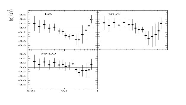
Figure 15: $h(x)$ extracted from CCFR’97 data for $xF_{3}$

The results of Table 2 demonstrate, that despite the correlation of the NLO values $\Lambda_{\overline{MS}}^{(4)}$ with the values of the twist-4 coefficient $A_{2}^{{}^{\prime}}$, the parameters of the adopted model for $xF_{3}(x,Q_{0}^{2})$ remain almost unaffected by the inclusion of the $1/Q^{2}$-term via the IRR-model of Ref. [82]. Thus, the corresponding parton distributions are less sensitive to twist-4 effects, than the NLO value of $\Lambda_{\overline{MS}}^{(4)}$. At the NNLO level the similar feature is related to already discussed tendency of the effective minimization of the $1/Q^{2}$- contributions to $xF_{3}$ (see also NNLO part of Fig. 15).

For the completeness the NLO and NNLO values of $\alpha_{\mathrm{S}}(M_{Z})$, obtained in Ref. [58] from the results of Table 2 with twist-4 terms modelled through the IRR approach are also presented:

$${\rm NLO}~{}~{}~{}\alpha_{\mathrm{S}}(M_{Z}) = 0.120\pm 0.003(stat)\pm 0.005(syst)^{+0.009}_{-0.007}$$ (23)

$${\rm NNLO}~{}~{}\alpha_{\mathrm{S}}(M_{Z}) = 0.118\pm 0.003(stst)\pm 0.005(syst)\pm 0.003$$

The systematical uncertainties in these results are determined by the pure systematical uncertainties of the CCFR’97 data for $xF_{3}$ [81]. The theoretical errors are fixed by variation of the factorization and renormalization scales [58]. The incorporation into the $\overline{MS}$-matching formula for $\alpha_{\mathrm{S}}$ [96, 97, 98] of the proposal of Ref. [52] to vary the scale of smooth transition to the world with $f=5$ number of active flavours from $m_{b}^{2}$ to $(6.5m_{b})^{2}$ was also taken into account. The theoretical uncertainties, presented in Eq. (2.6) are in agreement with the ones, estimated in Ref. [70] using the DGLAP equation. The NNLO value of $\alpha_{\mathrm{S}}(M_{Z})$ is in agreement with another NNLO result $\alpha_{\mathrm{S}}(M_{Z})=0.1172\pm 0.0024$, which was obtained in Ref. [99] from the analysis of SLAC, BCDMS, E665 and HERA data for $F_{2}$ with the help of the Bernstein polynomial technique [100].

2.7 Measuring Parton Luminosities and Parton Distribution Functions at the LHC

The traditional approach for cross section calculations and measurements at hadron colliders uses the proton–proton luminosity, $L_{proton-proton}$, and the “best” known quark, anti-quark and gluon parton–distribution functions, $PDF(x_{1},x_{2},Q^{2})$ to predict event rates $N_{events}$ for a particular parton parton process with a calculable cross section $\sigma_{theory}(q,\bar{q},g\rightarrow X)$, using:

$$N_{events}(pp\rightarrow X)=L_{proton-proton}\times PDF(x_{1},x_{2},Q^{2})\times\sigma_{theory}(q,\bar{q},g\rightarrow X).$$ (24)

The possible quantitative accuracy of such comparisons depends not only on the statistical errors, but also on the knowledge of $L_{proton-proton}$, the $PDF(x_{1},x_{2},Q^{2})$ and the theoretical and experimental uncertainties for the observed and predicted event rates for the studied process.

For many interesting reactions at the LHC one finds that statistical uncertainties become quickly negligible when compared to today’s uncertainties. Besides the technical difficulties to perform higher order calculations, limitations arise from the knowledge of the proton–proton luminosity and the parton distribution functions. Estimates for proton–proton luminosity measurements at the LHC assign typically uncertainties of $\pm$5%. Similar uncertainties are expected from the limited knowledge of parton distribution functions. Consequently, the traditional approach to cross section predictions and the corresponding measurements will be limited to uncertainties of at best $\pm$5%.

A more promising method [101], using only relative cross section measurements, might lead eventually to accuracies of $\pm$1%. The new approach starts from the idea that for high $Q^{2}$ processes one should consider the LHC as a parton–parton collider instead of a proton–proton collider. Consequently, one needs to determine the different parton–parton luminosities from experimentally clean and theoretical well understood reactions.

The production of the vector bosons $W^{\pm}$ and $Z^{0}$ with their subsequent leptonic decays fulfil these requirements. Taking today’s experimental results, the vector boson masses are precisely known and their couplings to fermions have been measured with accuracies of better than 1%. Furthermore, $W^{\pm}$ and $Z^{0}$ bosons with leptonic decays have 1) huge cross sections (several nb’s) and 2) can be identified over a large rapidity range with small backgrounds.

From the known mass and the number of “counted” events as a function of the rapidity $Y$ one can use the relations $M^{2}=sx_{1}x_{2}$ and $Y={1\over 2}ln\frac{x_{1}}{x_{2}}$ to measure directly the corresponding quark and anti-quark luminosities over a wide $x$ range (see fig.2). Simulation studies indicate that the leptonic $W$ and $Z$ decays can be measured with good accuracies up to lepton pseudorapidities $|\eta|<2.5$, corresponding roughly to quark and anti-quark $x$ ranges between 0.0003 to 0.1. The sensitivity of $W$ and $Z$ production data at the LHC even to small variations of the pdf’s is indicated in Figure 17.

Figure 16: a) The detected charged lepton cross section ratio, $\sigma(\ell^{+}\nu)/\sigma(\ell^{-}\bar{\nu})$, originating from the reaction $q\bar{q}\rightarrow W^{\pm}\rightarrow\ell^{\pm}\nu$ as a function of the lepton pseudorapidity for the MRS(H) and MRS(A) structure function parametrisation. b) The relative changes for the charged lepton distributions between the MRS(H) and MRS(A) parametrisations for $W^{+}$, $W^{-}$ and for $Z^{0}$ production [101].

Figure 17: The inclusive muon $p_{t}$ spectrum in selected photon–jet events originating from light and heavy quarks [105]. Assuming standard b–lifetime tagging expectations from ATLAS or CMS one should reduce the b–flavoured jets by about a factor of 2, the charm–jets by a factor of 10 and the light quarks by roughly a factor of 50.

Once the quark and anti-quark luminosities are determined from the $W$ and $Z$ data over a wide $x$ range, SM event rates of high mass Drell–Yan lepton pairs and other processes dominated by quark–anti-quark scattering can be predicted. The accuracy for such predictions is only limited by the theoretical uncertainties of the studied process relative to the one for $W$ and $Z$ production.

The approach can also be used to measure the gluon luminosity with unprecedented accuracies. Starting from gluon dominated “well” understood reactions within the SM, one finds that the cleanest experimental conditions are found for the production of high mass $\gamma$–Jet, $Z^{0}$–Jet and perhaps, $W^{\pm}$–Jet events. However, the identification of these final states requires more selection criteria and includes an irreducible background of about 10–20% from quark–anti-quark scattering. Some experimental observables to constrain the gluon luminosity from these reactions have been investigated previously [102]. The study, using rather restrictive selection criteria to select the above reactions with well defined kinematics, indicated the possibility to extract the gluon luminosity function with negligible statistical errors and systematics which might approach errors of about $\pm$1% over a wide $x$ range.

Furthermore, the use of the different rapidity distributions for the Vector bosons and the associated jets has been suggested in [103]. The proposed measurement of the rapidity asymmetry improves the separation between signals and backgrounds and should thus improve the accuracies to extract the gluon luminosity.

For this workshop, previous experimental simulations of photon–jet final states have been repeated with much larger Monte Carlo statistics and more realistic detector simulations [104]. These studies select events with exactly one jet recoiling against an isolated photon with a minimum $p_{t}$ of 40 GeV. With the requirement that, in the plane transverse to the beam direction the jet is back–to–back with the photon, only the photon momentum vector and the jet angle needs to be measured. Using the selected kinematics, the mass of the photon–jet system can be reconstructed with good accuracy. These studies show that several million of photon–jet events with the above kinematics will be detected for a typical LHC year of 10 fb^-1 and thus negligible statistical errors for the luminosity and $x$ between 0.0005 to $\approx$ 0.2. This $x$ range seems to be sufficient for essentially all high $Q^{2}$ reactions involving gluons. In addition, it might however be possible using dedicated trigger conditions, to select events with photon $p_{t}$ as low as 10–20 GeV, which should enlarge the $x$ range to values as low as 0.0001. The above reactions are thus excellent candidates to determine accurately the parton luminosity for light quarks, anti-quarks and gluons.

To complete the determination of the different parton luminosities one needs also to constrain the luminosities for the heavier $s$,$c$ and $b$ quarks. The charm and beauty quarks can be measured from a quark flavour tagged subsample of the photon–jet final states. One finds that the photon–jet subsamples with charm or beauty flavoured jets are produced dominantly from the heavy quark–gluon scattering ($c(b)g\rightarrow c(b)\gamma$). For this additional study of photon–jet final states, the jet flavour has been identified as being a charm or beauty jet, using inclusive high $p_{t}$ muons and in addition $b$-jet identification using standard lifetime tagging techniques [105]. The simulation indicates that clean photon–charm jet and photon–beauty jet event samples with high $p_{t}$ photons ($>$40 GeV) and jets with inclusive high $p_{t}$ muons. The muon $p_{t}$ spectrum from the different initial quark flavours is shown in Figure 17.

Assuming that inclusive muons with a minimum $p_{t}$ of 5–10 GeV can be clearly identified, a PYTHIA Monte Carlo simulation shows that a few 10⁵ $c$–photon events and about 10⁵ $b$–photon events per 10 fb^-1 LHC year should be accepted. These numbers correspond to statistical errors of about $\pm$ 1% for a $x_{c}$ and $x_{b}$ range between 0.001 and 0.1. However, without a much better understanding of charm and beauty fragmentation functions such measurements will be limited to systematic uncertainties of $\pm$ 5–10%.

Finally, the strange quark luminosity can be determined from the scattering of $sg\rightarrow Wc$. The events would thus consist of $W^{\pm}$ charm–jet final states. Using inclusive muons to tag charm jets and the leptonic decays of $W$’s to electrons and muons we expect about an accepted event sample with a cross section of 2.1 pb leading to about 20k tagged events per 10 fb^-1 LHC year. Again, it seems that the corresponding statistical errors are much smaller than the expected systematic uncertainties from the charm tagging of $\pm$ 5–10%.

In summary, we have identified and studied several final states which should allow to constrain the light quarks and anti-quarks and the gluon luminosities with statistical errors well below 1% for an $x$ range between 0.0005 to at $\approx$ 0.2. However, experimental systematics for isolated charged leptons and photons, due to the limited knowledge of the detector acceptance and selection efficiencies will be the limiting factor which optimistically limit the accuracies to perhaps $\pm$1% for light quarks and gluons. The studied final states with photon–jet events with tagged charm and beauty jets should allow to constrain experimentally the luminosities of $s$, $c$ and $b$ quarks and anti-quarks over a similar $x$ range and systematic uncertainties of perhaps 5–10%.

These promising experimental feasibility studies need now to be combined with the corresponding theoretical calculations and Monte Carlo modelling. In detail one has to study how well uncertainties from scale dependence, $\alpha_{\mathrm{S}}$ and higher order corrections change expected cross section ratios. Figure 6 gives an example of today’s uncertainties for $W$ and $Z$ cross sections at the LHC [10]. Similar estimates for all studied processes need to be done during the coming years in order to know the real potential of this approach to precision cross section measurements and their interpretation at the LHC.

2.8 Lepton Pair Production at the LHC and the Gluon Density in the Proton

The production of lepton pairs in hadron collisions $h_{1}h_{2}\rightarrow\gamma^{*}X;\gamma^{*}\rightarrow l\bar{l}$ proceeds through an intermediate virtual photon via $q{\bar{q}}\rightarrow\gamma^{*}$, and the subsequent leptonic decay of the virtual photon. Interest in this DY process is usually focused on lepton pairs with large mass $Q$ which justifies the application of perturbative QCD and allows for the extraction of the anti-quark density in hadrons [106]. Prompt photon production $h_{1}h_{2}\rightarrow\gamma X$ can be calculated in perturbative QCD if the transverse momentum $Q_{T}$ of the photon is sufficiently large. Because the quark-gluon Compton subprocess is dominant, $gq\rightarrow\gamma X$, this reaction provides essential information on the gluon density in the proton at large $x$ [28]. Alternatively, the gluon density can be constrained from the production of jets with large transverse momentum at hadron colliders [7].

In this report we exploit the fact that, along prompt photon production, lepton pair production is dominated by quark-gluon scattering in the region $Q_{T}>Q/2$. This realization means that new independent constraints on the gluon density may be derived from DY data in kinematical regimes that are accessible at the LHC but without the theoretical and experimental uncertainties present in the prompt photon case.

At LO, two partonic subprocesses contribute to the production of virtual and real photons with non-zero transverse momentum: $q\bar{q}\rightarrow\gamma^{(*)}g$ and $qg\rightarrow\gamma^{(*)}q$. The cross section for lepton pair production is related to the cross section for virtual photon production through the leptonic branching ratio of the virtual photon $\alpha/(3\pi Q^{2})$. The virtual photon cross section reduces to the real photon cross section in the limit $Q^{2}\rightarrow 0$.

The NLO corrections arise from virtual one-loop diagrams interfering with the LO diagrams and from real emission diagrams. At this order $2\rightarrow 3$ partonic processes with incident gluon pairs $(gg)$, quark pairs $(qq)$, and non-factorizable quark-anti-quark $(q\bar{q}_{2})$ processes contribute also. An important difference between virtual and real photon production arises when a quark emits a collinear photon. Whereas the collinear emission of a real photon leads to a $1/\epsilon$ singularity that has to be factored into a fragmentation function, the collinear emission of a virtual photon yields a finite logarithmic contribution since it is regulated naturally by the photon virtuality $Q$. In the limit $Q^{2}\rightarrow 0$ the NLO virtual photon cross section reduces to the real photon cross section if this logarithm is replaced by a $1/\epsilon$ pole. A more detailed discussion can be found in Ref. [107, 108].

The situation is completely analogous to hard photo-production where the photon participates in the scattering in the initial state instead of the final state. For real photons, one encounters an initial-state singularity that is factored into a photon structure function. For virtual photons, this singularity is replaced by a logarithmic dependence on the photon virtuality $Q$ [109].

A remark is in order concerning the interval in $Q_{T}$ in which our analysis is appropriate. In general, in two-scale situations, a series of logarithmic contributions will arise with terms of the type $\alpha_{\mathrm{S}}^{n}\ln^{n}(Q/Q_{T})$. Thus, if either $Q_{T}>>Q$ or $Q_{T}<<Q$, resummations of this series must be considered. For practical reasons, such as event rate, we do not venture into the domain $Q_{T}>>Q$, and our fixed-order calculation should be adequate. On the other hand, the cross section is large in the region $Q_{T}<<Q$. In previous papers [107, 108], we compared our cross sections with available fixed-target and collider data on massive lepton-pair production, and we were able to establish that fixed-order perturbative calculations, without resummation, should be reliable for $Q_{T}>Q/2$. At smaller values of $Q_{T}$, non-perturbative and matching complications introduce some level of phenomenological ambiguity. For the goal we have in mind, viz., constraints on the gluon density, it would appear best to restrict attention to the region $Q_{T}\geq Q/2$, but below $Q_{T}>>Q$.

We analyze the invariant cross section $Ed^{3}\sigma/dp^{3}$ averaged over the rapidity interval -1.0 $<y<$ 1.0. We integrate the cross section over various intervals of pair-mass $Q$ and plot it as a function of the transverse momentum $Q_{T}$. Our predictions are based on a NLO calculation [110] and are evaluated in the $\overline{\rm MS}$ renormalization scheme. The renormalization and factorization scales are set to $\mu=\mu_{R}=\mu_{F}=\sqrt{Q^{2}+Q_{T}^{2}}$. If not stated otherwise, we use the CTEQ4M parton distributions [111] and the corresponding value of $\Lambda$ in the two-loop expression of $\alpha_{\mathrm{S}}$ with four flavours (five if $\mu>m_{b}$). The DY factor $\alpha/(3\pi Q^{2})$ for the decay of the virtual photon into a lepton pair is included in all numerical results.

Figure 18: Invariant cross section $Ed^{3}\sigma/dp^{3}$ as a function of $Q_{T}$ for $pp\rightarrow\gamma^{*}X$ at $\sqrt{s}=14$ TeV.

Figure 19: Contributions from the partonic subprocesses $qg$ and $q\bar{q}$ to the invariant cross section $Ed^{3}\sigma/dp^{3}$ as a function of $Q_{T}$ for $pp\rightarrow\gamma^{*}X$ at $\sqrt{s}$ = 14 TeV. The $qg$ channel dominates in the region $Q_{T}>Q/2$.

In Fig. 19 we display the NLO cross section for lepton pair production at the LHC as a function of $Q_{T}$ for four regions of $Q$ chosen to avoid resonances, i.e.  from threshold to $2.5$ GeV, between the $J/\psi$ and the $\Upsilon$ resonances, above the $\Upsilon$’s, and a high mass region. The cross section falls both with the mass of the lepton pair $Q$ and, more steeply, with its transverse momentum $Q_{T}$. The initial LHC luminosity is expected to be 10³³ cm^-2 s^-1, or 10 fb^-1/year, and to reach the design luminosity of 10³⁴ cm^-2 s^-1 after three or four years. Therefore it should be possible to analyze data for lepton pair production to at least $Q_{T}\simeq 100$ GeV where one can probe the parton densities in the proton up to $x_{T}=2Q_{T}/\sqrt{s}\simeq 0.014$. The UA1 collaboration measured the transverse momentum distribution of lepton pairs at $\sqrt{s}=630$ GeV to $x_{T}=0.13$ [112], and their data agree well with our expectations [107, 108].

The fractional contributions from the $qg$ and $q\bar{q}$ subprocesses through NLO are shown in Fig. 19. It is evident that the $qg$ subprocess is the most important subprocess as long as $Q_{T}>Q/2$. The dominance of the $qg$ subprocess increases somewhat with $Q$, rising from over 80 % for the lowest values of $Q$ to about 90 % at its maximum for $Q\simeq$ 30 GeV. Subprocesses other than those initiated by the $q\bar{q}$ and $qg$ initial channels are of negligible import.

The full uncertainty in the gluon density is not known. We estimate the sensitivity of LHC experiments to the gluon density in the proton from the variation of different recent parametrizations. We choose the latest global fit by the CTEQ collaboration (5M) as our point of reference [7] and compare results to those based on their preceding analysis (4M) [111] and on a fit with a higher gluon density (5HJ) intended to describe the CDF and D0 jet data at large transverse momentum. We also compare to results based on global fits by MRST [28], who provide three different sets with a central, higher, and lower gluon density, and to GRV98 [113].

Figure 20: Invariant cross section $Ed^{3}\sigma/dp^{3}$ as a function of $Q_{T}$ for $pp\rightarrow\gamma^{*}X$ at $\sqrt{s}=14$ TeV in the region between the $J/\psi$ and $\Upsilon$ resonances. The largest differences from CTEQ5M are obtained with GRV98 (minus 18 %).

In Fig. 20 we plot the cross section for lepton pairs with mass between the $J/\psi$ and $\Upsilon$ resonances at the LHC in the region between $Q_{T}=50$ and 100 GeV ($x_{T}=0.007\dots 0.014$). For the CTEQ parametrizations we find that the cross section increases from 4M to 5M by 5 % and does not change from 5M to 5HJ in the whole $Q_{T}$-range. The largest differences from CTEQ5M are obtained with GRV98 (minus 18 %).

The theoretical uncertainty in the cross section can be estimated by varying the renormalization and factorization scale $\mu_{R}=\mu_{F}$ about the central value $\sqrt{Q^{2}+Q_{T}^{2}}$. In the region between the $J/\psi$ and $\Upsilon$ resonances, the cross section drops from $\pm 39\%$ (LO) to $\pm 16\%$ (NLO) when $\mu$ is varied over the interval interval $0.5<\mu/\sqrt{Q^{2}+Q_{T}^{2}}<2$. The $K$-factor ratio (NLO/LO) is approximately 1.3 at $\mu/\sqrt{Q^{2}+Q_{T}^{2}}=1$.

We conclude that the hadroproduction of low mass lepton pairs is an advantageous source of information on the parametrization and size of the gluon density. With the design luminosity of the LHC, regions of $x_{T}\simeq 0.014$ should be accessible. The theoretical uncertainty has been estimated from the scale dependence of the cross sections and found to be small at NLO.

3 MONTE CARLO EVENT GENERATORS

The event generation package is the first link of the event simulation/reconstruction software suite which is central to any experimental data analysis. Physics results are obtained by a direct comparison of simulated and observed data. Therefore, precision analyses rely on an accurate and detailed implementation of the underlying physics model in the generation of signal as well as background processes.

An event generator is built from various pieces whose object and nature are quite different. Some are perturbative: the hard-scattering matrix element (ME) which can be calculated exactly, the parton shower (PS) which approximates, through the evolution equations, the initial parton conditions and final-state jet structure, and some are non-perturbative and probabilistic like the parton distribution in the composite initial particles and the fragmentation of the final partons. The main difficulty in writing event generator programs lies on the consistent matching of those different components.

Several multi-process parton shower event generators (PSEG) have been developed to cover the physics programme at $e^{+}e^{-}$, $pp$ or $p\bar{p}$ colliders: Pythia [115], Herwig [116, 117, 118], Isajet [119, 120]. These Monte Carlo programs provide an accurate description of jet physics at existing high-energy colliders, which allow the simulation of a large variety of final-state processes within and beyond the SM. These programs have been essential to demonstrate the impressive LHC potential on many different and detailed physics questions, to develop new analysis strategies and also to optimize the performance of the LHC experiments.

Nevertheless, the increasing potential of very accurate measurements at the LHC and the sensitivity to exotic physics processes using specific and rare kinematics demand for the implementation of higher-order processes and thus a rethinking of the organisation and probably an extensive rewriting of many specific Monte Carlo generators.

In the first section, we list the major points of concern or pending issues in the development of event generators for the LHC physics. The next section discusses the present treatments of minimum bias and underlying events. The following two contributions address the implementation of transverse momentum effects in boson production. The last three sections present a short description of some of the currently available ME generators.

3.1 QCD event generators: major issues

3.1.1 Multi-particle final states

Matrix element

PSEG are essentially limited to the simulation of $2\rightarrow 2$ processes based on analytic matrix element expressions. However, the LHC center of mass energy is large enough to open many high multiplicity channels. In addition, new particle searches in the Higgs and Susy sectors require the simulation of $2\rightarrow 4$, $2\rightarrow 6$ or even $2\rightarrow 10$ jet processes for which a precise knowledge of the SM background processes is mandatory.

QCD multi-jets events $pp\rightarrow n_{1}$ jets and $pp\rightarrow Z/W+n_{2}$ jets have been computed at LO, for $n_{1}\leq 6$ by using the SPHEL approximation [121] (i.e. assuming all helicity amplitudes give similar contributions), and for $n_{1}\leq 6$ (Njets) [122] and $n_{2}\leq 4$ (Vecbos) [123] by using exact recurrence relations [124].

In the PSEG, partonic final states are mimicked through the PS mechanism based on the leading logarithmic (LL) approximation. It properly describes parton radiations only in the soft and collinear region leading to a crude estimate of the multi-parton dynamics of the event. The remedy for a better multi-parton event generator is two-fold: (i) to improve the simulation of the PS by introducing ME corrections (see Sects. 3.3 and 3.4), (ii) to implement the complete multi-parton hard scattering ME process.

The evaluation of ME for multi-particle QCD processes has been reviewed in [125]. A powerful technique is the use of helicity amplitudes in the massless limit [126, 127, 128]. Recent developments in this direction were done in [129] where the Weyl-van-der-Waarden spinor calculus was generalized to the massive fermions. At this level of complexity where so many sub-processes must be calculated, the analytic hand-made approach becomes literally intractable unless stringent approximations are imposed, as the narrow width approximation, massless fermions, averaging/summing over initial/final helicity state or selecting only a subset of gauge invariant diagrams.

A more systematic approach is needed: (i) to provide all required channels, (ii) to allow for a detail study of finite width effects and helicity and color correlations, (iii) to generate complete ME expressions in order to match the experimental precision. For example, the LHC statistics will allow to measure the top quark mass with negligible uncertainty. This implies that both top quark and $W$ finite widths must be taken into account in the evaluation of the interference between signal and background diagrams.

The automatic Feynman diagram generator packages, largely used for the $e^{+}e^{-}$ physics analysis, generate complete and approximation-free tree-level ME codes, in principle, for any final state multiplicity and with a higher reliability level than hand written procedures. They are gradually upgraded to $pp$ physics. Grace [130, 131, 132], Madgraph [133], Alpha [134] and Phact [135, 136] are based on tree level helicity amplitude algorithms in arbitrary massive gauge theories. The evaluation is purely numerical and the code size scales linearly with the number of external particles. In Alpha (see Sect. 3.7), an iterative algorithm, based on Green functional methods, evaluates the amplitudes for any given Lagrangian and leads to more compact expressions allowing, for example, the generation of $gg/q\bar{q}\rightarrow n$ with $n\leq 9$ [137]. The CompHEP [138, 132] package is based on the squared amplitude technique. Here, the size of the ME code grows exponentially with the number of external particles, but it produces more powerful symbolic expressions. This method has shown good efficiency for the evaluation $2\rightarrow 3,4$ processes, comparable to the helicity amplitude algorithms.

However, the completeness of the automatically produced matrix elements and the poor optimization of the code (when compared to hand coding) often translate into computationally intensive and memory hungry expressions, sometimes reaching the limit of computability on conventional workstations.

The development effort is focused on two directions: (i) to improve the code efficiency by the introduction of new computational algorithm, by a better optimization and by the “automated” introduction of approximations, (ii) to develop code taking advantage of massively parallel systems [139, 140].

Multi-dimensional integration

The cross section computation and the event generation stage are based on the multi-dimensional integration procedure. It needs to be focused to the phase space region where the amplitude is large. The amplitude behavior on those regions can be sharp and multi-variate due to complex singularity patterns. Integration packages including Vegas [141, 142], Bases/Spring [143, 144], MILXy [145], Foam [146] use self-adapting techniques based on importance and/or stratified sampling. However, a faster integration convergence is obtained by providing the integration algorithm with information on the location and behavior of the singularities. This is usually done by the so-called “kinematics” routine performing the mapping of the integration variables to the physics parameters. Not yet fully automated [147], it is aiming by appropriate variable transforms at smoothing the singularities and reducing their dimensionality.

For many important processes, it is impossible to match all singularities within a single set of variable transforms (e.g. $pp\rightarrow u\bar{u}d\bar{d}$ with $W$,$Z$ decays and $t$-channel singularities). In those cases, one relies on a multichannel algorithm [148, 149] where each peaking structure has its own appropriate mapping.

Interface to the PSEG package

The implementation of automatically-produced hard-process ME in PSEG is a delicate but essential task to benefit from the implementation of the complex QCD machinery reproducing the initial and final states.

The ultimate goal is to embed the full ME with its appropriate kinematics mapping into the kernel of the PSEG through some automated procedure. Although some progress has been achieved toward this end, a simpler approach is to generate parton level event sample using a program dedicated to a given ME, then let them fragment through the PS and hadronization scheme of the selected PSEG. For example, in Pythia the routines PYUPIN and PYUPEV are available for the implementation of externally produced event processes. Similar facilities exist or can be implemented in other PSEG. This technique already used by the LHC experiments (see section 3.5) may raise consistent parameter and parton distribution bookkeeping issues.

3.1.2 Heavy-quark production and parton shower

Keeping the fermion masses at their on-shell value, although making the expressions more complex, is always a good practice to get rid of the propagator pole divergence. At LHC, from a phenomenological point of view, light $u$, $d$ and $s$ quark masses can be neglected, but heavy $c$, $b$ and $t$ quark should be implemented not only to reproduce threshold effects, but also for a correct treatment of spin correlation and NLO corrections. Beside the basic $t$-quark physics studies, the heavy-quark event generation plays an important role as the dominant background to the Higgs search ($W/Zb\bar{b}$, $t\bar{t}+2jets$ and $t\bar{t}t\bar{t}$, $b\bar{b}b\bar{b}$, $b\bar{b}t\bar{t}$). Those computations require the use of multi-particle massive ME as developed in the automatic approach.

The simulation of the PS developed by a massive quark is similar to the massless case above an angular cut-off of $\theta=m_{q}/E_{q}$, while below no radiation is emitted. This is true only in the soft and collinear region, if the physics observable is sensitive to high-$p_{T}$ effects (e.g. top mass reconstruction) full massive radiative heavy-quark decay ME (i.e. $t\rightarrow bWg$) must be embedded in the PS code [150, 151].

3.1.3 Color and helicity implementation

Color and spin effects are important at LHC. Color correlations beside driving the fragmentation of partons lead to color reconnection effects acting on the local event multiplicity. Spin effects in the top physics, for example, provide a useful handle on the nature of the couplings [152].

The procedure to assign helicity and color to the initial/final partons requires similar implementations in an event generator. For $2\rightarrow 2$ processes, the number of possible color flows is small and can be handled easily through an overall factor for the single diagram case and through a slightly more elaborated treatment when dealing with the interference of 2 diagrams with different color flows [153]. For higher multiplicity [154], in the super-symmetric QCD [155] and in the $R$-parity violated processes [156], the selection of the color final state is more involved. In the helicity amplitude approach, each diagram must be decomposed over a color flow reference base. The cross sections for all possible color/helicity combinations ($8^{n_{g}}\times 3^{n_{q}}\times 2^{n_{g}+n_{q}}$) are then evaluated. Adding more final-state particles drastically increases the number of cross section computations.

3.1.4 NLO and NNLO corrections

In QCD, talking about corrections concerning the NLO and NNLO contributions is an understatement. Higher-order computations are very important not only due to the rather large coupling constant $\alpha_{s}$ inducing substantial corrections, but mainly because they reduce the renormalization and factorization scale dependence. Furthermore, analysis or experimental-cut dependencies (like the cone-size dependence in jet analysis) are better reproduced when higher-order corrections are included. Roughly speaking if one can say that NLO is the first order giving a sensible perturbative result, NNLO can be seen as the error estimate on this result.

In principle, computing NLO matrix elements is straightforward using loop integral reduction techniques, but the number of involved diagrams and their complexity have lead to the development of automatic coding programs like FeynArt/FeynCalc Formcalc/Looptools [157, 158, 159] or Grace (see Sect. 3.6). The latter is geared to provide 1-loop $n$-body final-state ME while, in practice, a maximum of $n=4$ and further approximations are imposed by computational limitations.

But the main problem lies in the cancellation of soft and collinear infinities present at NLO precision. Fully inclusive computations generate the so-called $K$-factor as a global scaling factor, but detailed analyses need phase-space dependent corrections. Two techniques (see the general discussion in Sect. 4) have been developed to handle the cancellations: the phase-space slicing method [160] and the subtraction method [161, 162]. In the former, the cancellation is performed by approximate integration within regions delimited by some unphysical cut-off (the approximation becomes better as the cut-off becomes smaller), in the latter the divergent terms are replaced by a suitable analytically-integrable expression plus its finite difference with the original expression. For these two approaches, Monte-Carlo integration techniques are used, allowing for a precise implementation of the experimental cuts. These NLO programs (see Sect. 4) can be seen as “pseudo-event generators”. Phase space points (pseudo-events) after being tested against the cuts have their corresponding weights accumulated to form the observable. Single or multi differential distributions can be built in one go. But two issues prevent the use of these packages as true event generators: (i) the handling of negative weighted events and (ii) the interface to the PS and fragmentation stage. No definite scheme currently exists to properly implement LO+NLO processes in a stochastic event generator.

The negative weighted events arise from the virtual corrections cancelling the soft and collinear divergences. Several attempts are on trial. One approach is to treat those events as the usual positive weighted events and to observe the cancellation only after the reconstruction stage where the experimental resolution will have introduced a natural cut-off. This implies the generation, the simulation and the reconstruction of many events which finally cancel, not contributing to the statistical significance and therefore leads to unstable results. More advanced attempts have been based on a re-weighting of event generated by showering from the LO matrix elements  [163, 164, 165, 166, 150, 151]. Recently, a modified subtraction method is exercised to built NLO event generators [167, 168] by point-by-point cancellation of the singularities. This approach looks quite encouraging although final implementations have not been realized yet.

The second problem is the matching of a NLO ME to the PS. A consistent approach would be to interface a NLO ME to next-to-leading logarithmic (NLL) order parton shower, but no such algorithm exist yet (see Sect. 3.1.5) and therefore one has to find the least damaging approach to connect NLO ME and LL PS and final hadronization. Basically the ordered evolution PS variable should be matched to the ME regularization parameter. Remaining double counting effects will be removed by the rejection algorithm for each event topology [167].

3.1.5 Parton shower

In hadronic collision, the parton showering occurs both in the initial and in the final state. In the latter, the high-virtuality partons are evolved using the DGLAP equations down to quasi-real objects ready to undergo final hadronization. The initial partons selected from the parton distribution functions with a relative momentum fraction $x$ and virtuality $Q^{2}$ follow a backward evolution [169, 170, 171] to bring back the virtuality down to values compatible with the confinement of partons in a fast hadron (cloud of quasi-real particles). In this process, gluons and quarks are emitted (absorbed in the backward-evolution time frame) by quark radiation or gluon splitting. This radiation contributes to the final-state multiplicity (beam remnants). In addition, the parton acquires a transverse momentum and the full kinematic of the initial centre-of-mass of the hard scattering will be uniquely defined (see Sects. 3.3 and 3.4).

The parton shower model implemented in the PSEG is essentially a LL approximation, even if some NLL corrections have been added through exact energy-momentum conservation, angular ordering and ‘optimal scheme’ definition for $\alpha_{\mathrm{S}}$ [172]. The dominant logarithmic singularities are resummed in the Sudakov form factors.

As seen in the previous section, the need for a NLL parton shower is high. The problem is that resumming higher-order correction breaks one major “raison d’être” of the PS: the universality. At LL level, the hard scattering and the parton showering are 2 independent processes (factorization between the short an the long range) and the success of the PSEG is based on this feature. Incorporating higher-order corrections may break universality and each type of hard scattering process may require a specific NLL PS evaluation (see also the last paragraph in Sect. 3.6).

3.1.6 Multi-parton scattering

PSEG for rare events usually include single-scattering processes only. At the LHC, one expect, due to the unitary bound, multi-parton interactions to give important contributions to several processes [173, 174]. As an example the cross section for the production of four jets with double-parton collisions dominates the single-scattering process when the minimum of the produced jets transverse momenta is $p_{t_{min}}<20\,$GeV (see Sect. 8). These processes, observed by CDF [175, 176], are largely discussed in Sect. 8, in the Bottom Production Chapter of this Report and in the ATLAS TDR [1]. Information related to the PSEG implementation of multi-parton scattering can be found in the Pythia [115] and Herwig v6.1 [118] manuals.

Under the simplifying assumptions of no correlation between the longitudinal-momentum fractions of the initial partons, and of the process-independence of parton correlations in transverse-momentum space, double-parton interactions are easyly implementable into PSEG codes, in terms of a single universal parameter $\sigma_{eff}$ (see Sect. 8). However, none of those hypotheses can be taken for granted. It is therefore important to implement those effects in PSEG programs by using different dynamical models. In addition to their contributions to the background to new particle searches, the multi-parton interactions at the LHC can provide insights on the dynamical structure of the hadrons [177, 178, 179].

3.1.7 Standardization and language issues

The availability of several independent event generation packages although aiming at similar scopes is a big advantage for the experimental community. It makes possible comparative checks and leads to a deeper understanding of the various approximations used and implementation dependent issues.

However, one must strongly stress that the definition of a common interface scheme between the event generators and the simulation/analysis experimental packages would be extremely valuable. Such a standardization would cover the following issues: (i) parameter naming convention, (ii) parameter database management, (iii) event output format, (iv) event sample database.

Although the standardization scheme can already be exercised on the existing Fortran PSEG, it takes its full meaning with the current transition to the object oriented (OO) methodology. The maintenance issue of those large and complex packages over the long expected lifetime of the LHC experiments is the main reason for using the OO technology, but the built-in object modularity opens the door to a finer grained standardization at least to the level of the interfaces of the main procedures (random number generator, diagram generation, diagram display, matrix element code, integrator, parton shower, fragmentation, structure functions). This would allow the building of event generators using procedures from various origins. Most of the PSEG package developers have endorsed C++ as the language for the future developments. Design and implementation studies are already in progress [180, 181, 182].

On these last issues, the setting up of a dedicated working group with all concerned authors and users would be quite timely.

3.2 Minimum bias and underlying events

A crucial area of physics for the LHC is the structure of finals states in soft minimum-bias collisions and the soft underlying event in hard processes. At present very little is understood about these matters on the basis of QCD starting from first principles. The three principal event generators in use for LHC physics, Isajet, Herwig and Pythia, use quite different models for this type of physics, although each uses basically the same model to generate both minimum-bias and underlying events.

Simulation of minimum-bias events starts with a parametrization of the total cross section. Herwig and Pythia both use the Donnachie-Landshoff fit [183]

$$\sigma_{tot}=21.70s^{0.0808}+56.08s^{-0.4525}$$

(where $\sigma$ is in mb and $\sqrt{s}$ in GeV), whereas Isajet uses a $\log^{2}s$ form:

$$\sigma_{tot}=25.65\left[1+0.0102\log^{2}(s/1.76)\right]\;.$$

Notice (see Fig. 21) that, although smaller asymptotically, the Isajet value is larger at LHC energies.

Figure 21: The $pp$ total cross section according to the parametrizations used in Herwig, Pythia and Isajet.

To model soft final states, Herwig uses the UA5 minimum-bias Monte Carlo [184], adapted to its own cluster fragmentation model. See the Herwig manuals [118] for further details. The model is based on a negative binomial parametrization of the overall charged multiplicity. This has the property of generating large multiplicity fluctuations with long range in rapidity, in addition to short-range correlations due to cluster decay. For true minimum-bias simulation, the soft events generated by Herwig should be mixed with an appropriate fraction of QCD hard-scattering events. For the underlying event in hard collisions, the same model is used to simulate a soft collision between beam clusters containing the spectator partons.

The minimum-bias/underlying event model used in Isajet is based on a mechanism of multiple Pomeron exchange [185], with a fluctuating number of ‘cut Pomerons’ acting as sources of final-state hadrons. Each cut Pomeron fragments directly into hadrons according to the Isajet independent fragmentation model, with the fragmentation axis along the beam direction. The model again produces large long-range multiplicity fluctuations, but short-range correlations are weak due to the absence of clustering.

In Pythia a multiple interaction model is used to generate hard, soft and underlying events in a unified manner. Multiple interactions are discussed in more detail below. The number $n$ and distribution $P(n)$ of interactions per event is controlled by the minimum transverse momentum allowed in each interaction and, optionally, by a model for the impact parameter profile. Long-range fluctuations may be somewhat weaker in this model, with short-range correlations somewhere between the two other generators. In minimum-bias events the choice $n=0$ can occur, in which case a two-string fragmentation model linking a quark in each beam proton to a diquark in the other is used.

A study of energy-flow correlations between well-separated phase-space regions would be helpful in understanding the underlying event and in separating its contribution from that of the hard subprocess [186]. Such a study is currently being undertaken by the CDF Collaboration.

3.3 Matrix-element corrections to vector boson production and transverse-momentum distributions

Vector boson production will be a fundamental process to test QCD and the SM of the electroweak interactions. Monte Carlo event generators [115, 116, 117] simulate the initial-state radiation in vector boson production processes in the soft/collinear approximation, but can have ‘dead zones’ in phase space, where no parton emission is allowed. The radiation in the dead zone is physically suppressed, since it is not soft or collinear logarithmically enhanced, but not complete absent as nevertheless happens in standard PS algorithms. Matrix-element corrections to the Herwig simulation of Drell–Yan processes have been implemented in [164] following the method described in [163]: the dead zone is populated by the using of the exact first-order amplitude and the cascade in the already-populated phase-space region is corrected using the exact matrix element every time an emission is capable of being the hardest so far. A somewhat different procedure is followed to implement matrix-element corrections to the Pythia event generator [165, 166]: the PS probability distribution is applied over the whole phase space, the previous algorithm having a cut $q_{T}<m_{V}$ on the vector boson $V$ transverse momentum to avoid double counting, and the exact ${\cal O}(\alpha_{S})$ matrix element is used only to generate the closest branching to the hard vertex.

Figure 22: $W$ transverse momentum distribution at the LHC, according to Herwig before (dotted line) and after matrix-element corrections (solid).

Figure 23: Comparison of the DØ data with Herwig 6.1 for $q_{T{\mathrm{int}}}=0$ (solid) and 1 GeV (dashed).

Referring hereinafter to the Herwig event generator, in Fig. 23 the distribution of the $W$ transverse momentum $q_{T}$ is plotted at the LHC by running Herwig 5.9, the latest public version, and Herwig 6.1 [118], the new version including matrix-element corrections to vector boson production, for an intrinsic transverse momentum $q_{T{\mathrm{int}}}=0$, its default value. A big difference can be seen at large $q_{T}$, where the 6.1 version has many more events which are generated via the exact ${\cal O}(\alpha_{S})$ amplitude. In the PS soft/collinear approximation, on the contrary, $q_{T}$ is constrained to be $q_{T}<m_{W}$. A suppression can be seen at small $q_{T}$, due to the fact that, even though we are providing the Monte Carlo shower with the tree-level ${\cal O}(\alpha_{S})$ matrix-element corrections, virtual contributions are missing and, by default, we still get the total leading-order cross section. No next-to-leading order parton shower algorithm is presently available.

In Fig. 23 some recent DØ data [187] on the $W$ $q_{T}$ spectrum at the Tevatron is compared with the Herwig 6.1 results, which are corrected for detector smearing effects. A good agreement is found after hard and soft matrix-element corrections; the options $q_{T}=0$ and 1 GeV are investigated, but no relevant effect is visible after detector corrections, which have been shown in [164] to be pretty strong.

Figure 24: Comparison of the CDF data on $Z$ production with Herwig 5.9 (dotted line) and Herwig 6.1 for $q_{T{\mathrm{int}}}=0$ (solid), 1 GeV (dashed) and 2 GeV (dash-dotted).

Figure 25: Ratio of the $W$ and the $Z$ $q_{T}$ distributions, according to Herwig 6.1 for $q_{T{\mathrm{int}}}=0$ (solid), 1 GeV (dashed) and 2 GeV (dotted).

In Fig. 25, we compare Herwig with some CDF data [188] on $Z$ production, already corrected for detector effects, which are however much smaller than the $W$ case. We consider the options $q_{T{\mathrm{int}}}=0$, 1 and 2 GeV. The overall agreement is good, with a crucial role of matrix-element corrections to fit in with the data at large $q_{T}$. At low $q_{T}$, the best fit is the one corresponding to $q_{T{\mathrm{int}}}=2$ GeV. Even though, as can be seen from Fig. 25, the $Z$ distribution is strongly dependent on the intrinsic transverse momentum at low $q_{T}$, in [189] and in Fig. 25 it is shown that the ratio of the $W$ and $Z$ differential cross sections, both normalized to one, is roughly independent of $q_{T{\mathrm{int}}}$, which means that the effect of a non-zero $q_{T{\mathrm{int}}}$ is approximately the same for both $W$ and $Z$ spectra. This ratio is one of the main inputs for the experimental analyses and the fact that it is not strongly dependent on unknown non-perturbative effects is good news for studies on the $W$ mass measurement.

It is also worthwhile comparing the Herwig 6.1 $q_{T}$ distributions with some available calculations which resum the logarithms $l=\log(m_{V}/q_{T})$, $m_{V}$ being the vector boson mass, in a Sudakov-like exponential form factor (see Sect. 5 for a review of theoretical aspects of Sudakov resummation). Such logarithms are large in the low $q_{T}$ range. In [164] the Monte Carlo results are compared with the resummation approaches of [190], where all terms down to the next-to-leading logarithmic order $\approx\alpha_{S}^{n}l^{n}$ are kept in the Sudakov exponent, both in $q_{T}$- and impact parameter $b$-space, and of [191], where the authors expand the Sudakov exponent and keep in the differential cross section all terms down to the order $\approx\alpha_{S}^{n}l^{2n-3}$, which are next-to-next-to-leading logarithms after the expansion of the form factor. Such resummations are also matched to the exact first-order result in [164]. In Figs. 27 and 27 the $W$ $q_{T}$ distributions are plotted according to Herwig 6.1 and the resummed calculations at small $q_{T}$ and over the whole $q_{T}$ range respectively. The overall agreement at low $q_{T}$ is reasonable and the Herwig plots lie well within the range of the resummed approaches. At large $q_{T}$ the matching of the resummed calculations to the exact ${\cal O}(\alpha_{S})$ result works well only for the approach of [190] in the $q_{T}$-space, as we have a continuous distribution at the point $q_{T}=m_{W}$, the other distributions showing a step due to uncompensated contributions of order $\alpha_{S}^{2}$ or higher.

In [164], it is also shown that matrix-element corrections to vector boson production have a negligible effect on rapidity distributions, the latest version Herwig 5.9 agreeing well with the CDF data on the $Z$ rapidity. The implemented hard and large-angle gluon radiation has nevertheless a marked impact on jet distributions both at the Tevatron and LHC, as many more events with high transverse energy jets are now generated.

Figure 26: The $W$ $q_{T}$ distribution in the low $q_{T}$ range at the Tevatron, according to Herwig 6.1, for $q_{T{\mathrm{int}}}=0$ (solid histogram) and 1 GeV (dashed histogram), compared with the resummed results of [190] in $q_{T}$- (solid line) and $b$-space (dotted line) and of [191] in the $q_{T}$-space.

Figure 27: As in Fig. 27, but over the whole $q_{T}$ spectrum.

While these analyses are performed assuming that the produced vector boson decays into a lepton pair, the implementation of matrix-element corrections to the Herwig simulation of the hadronic $W$ decay $W\rightarrow q\bar{q}^{\prime}$ is in progress, however it is expected to be a reasonably straightforward extension of the corrections already applied to the process $Z\rightarrow q\bar{q}$. Furthermore, the method applied to improve the initial-state shower for $W/Z$ production could be extended to many other processes which are relevant for the LHC. Among these, we expect that the implementation of matrix-element corrections to top and Higgs production may have a remarkable phenomenological effect at the LHC. This is in progress as well.

3.4 A comparison of the predictions from Monte Carlo programs and transverse momentum resummation

For many physical quantities, the predictions from PS Monte Carlo programs should be nearly as precise as those from analytic theoretical calculations. This is expected, among others, for calculations which resum logs with the transverse momentum of partons initiating the hard scattering (resummed calculations are described in Sect. 5). In the recent literature, most calculations of this kind are either based on or originate from the formalism developed by J. Collins, D. Soper, and G. Sterman [192], which we choose as the analytic ‘benchmark’ of this Section. In this case, both the Monte Carlo and analytic calculations should accurately describe the effects of the emission of multiple soft gluons from the incoming partons, an all orders problem in QCD. The initial state soft gluon emission can affect the kinematics of the final state partons. This may have an impact on the signatures of physics processes at both the trigger and analysis levels and thus it is important to understand the reliability of such predictions. The best method for testing the reliability is the direct comparison of the predictions to experimental data. If no experimental data is available for certain predictions, then some understanding of the reliability may be gained from the comparison of the predictions from the two different methods.

Parton showering resums primarily the leading logarithms, which are universal, i.e. process independent, and depend only on the given initial state. In this lies one of the strengths of Monte Carlos, since parton showering can be incorporated into a wide variety of physical processes. As discussed in Sect. 5, an analytic calculation, in comparison, can resum all large logarithms, since all (in principle) are included in the Sudakov exponent given in Eq. (48).

If we try to interpret parton showering in the same language as resummation, which is admittedly risky, then we can say that the Monte Carlo Sudakov exponent always contains terms analogous to $A^{(1)}$ and $B^{(1)}$ in Eq. (49). It was shown in Ref. [172] that a suitable modification of the Altarelli–Parisi splitting function, or equivalently the strong coupling constant $\alpha_{s}$, also effectively approximates the $A^{(2)}$ coefficient. 

Both Monte Carlo and analytic calculations describe the effects of the emission of multiple soft gluons from the incoming partons, an all orders problem in QCD. The initial state soft gluon emission affects the kinematics of the final state partons, which, in turn, may have an impact on the signatures of physics processes at both the trigger and analysis levels. Thus it is important to understand the reliability of such predictions. The best method for testing the reliability is the direct comparison of the predictions to experimental data. If no experimental data is available for certain predictions, then some understanding of the reliability may be gained from the comparison of the predictions from the two different methods.

In particular, one quantity which should be well–described by both calculations is the transverse momentum ($p_{T}$) of the final state electroweak boson in a subprocess such as $q\overline{q}\rightarrow WX$, $ZX$ or $gg\rightarrow HX$, where most of the $p_{T}$ is provided by initial state parton showering. The parton showering supplies the same sort of transverse kick as the soft gluon radiation in a resummation calculation. This correspondence between the Sudakov form factors in resummation and Monte Carlo approaches may seem trivial, but there are many subtleties in the relationship between the two approaches relating to both the arguments of the Sudakov factors as well as the impact of sub–leading logs [166, 188, 164].

At a point in its evolution corresponding to (typically) the virtuality of a few GeV², the parton shower is cut off and the effects of gluon emission at softer scales must be parameterized and inserted by hand. This is similar to the (somewhat arbitrary) division between perturbative and non–perturbative regions in a resummation calculation. The parametrization is typically done with a Gaussian smearing similar to that used for the non–perturbative $k_{T}$ in a resummation program. In general, the value for the non–perturbative $\langle k_{T}\rangle$ needed in a Monte Carlo program will depend on the particular kinematics being investigated. 

A value for the average non–perturbative $k_{T}$ greater than 1 GeV does not imply that there is an anomalous intrinsic $k_{T}$ associated with the parton size; rather, this amount of $\langle k_{T}\rangle$ needs to be supplied to provide what is missing in the truncated parton shower. If the shower is cut off at a higher virtuality, more of the ‘non–perturbative’ $k_{T}$ will be needed.

3.4.1 Vector boson production and comparison with Pythia and Resbos

The (resolution corrected) $p_{T}$ distribution for $Z^{0}$ bosons (in the low $p_{T}$ region) for the CDF experiment [188] is shown in Figure 28 [193], compared to both the resummed prediction from ResBos[194], and to two predictions from Pythia (version 6.125). One Pythia prediction uses the default (rms) value of intrinsic $k_{T}$ of 0.44 GeV and the second a value of 2.15 GeV per incoming parton. The latter value was found to give the best agreement for Pythia with the data.  All of the predictions use the CTEQ4M parton distributions [111]. Good agreement is observed between ResBos, Pythia and the CDF data.

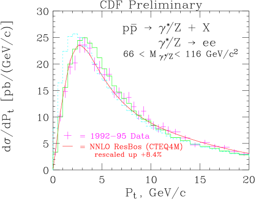
Figure 28: The $Z^{0}$ $p_{T}$ distribution (at low $p_{T}$) from CDF for Run 1 compared to predictions from ResBos and from Pythia. The two Pythia predictions use the default (rms) value for the non–perturbative $k_{T}$ (0.44 GeV) and the value that gives the best agreement with the shape of the data (2.15 GeV).

3.4.2 Higgs boson production and comparison with Pythia

A comparison of the Higgs $p_{T}$ distribution at the LHC [193], for a Higgs mass of 150 GeV, is shown in Figure 29, for ResBos [195] and the two recent versions of Pythia. Pythia has been rescaled to agree with the normalization of ResBos to allow for a better shape comparison. Note that the peak of the resummed distribution is at $p_{T}\approx$ 11 GeV (compared to about 3 GeV for $Z^{0}$ production at the Tevatron). This is partially due to the larger mass (150 GeV compared to 90 GeV), but is primarily because of the larger color factors associated with initial state gluons ($C_{A}=3$) rather than quarks ($C_{F}=4/3$), and also because of the larger phase space for initial state gluon emission at the LHC.

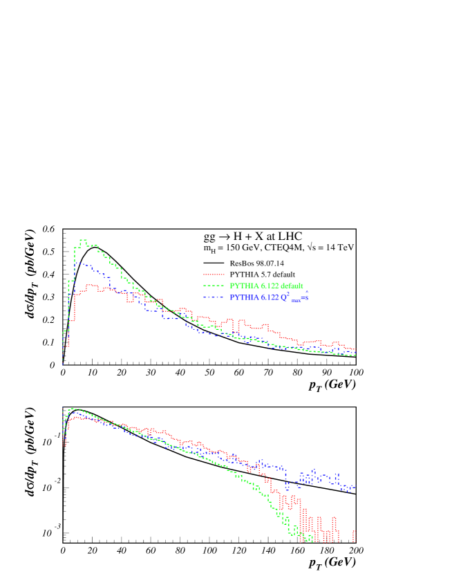
Figure 29: A comparison of predictions for the Higgs $p_{T}$ distribution at the LHC from ResBos and from two recent versions of Pythia. The ResBos and Pythia predictions have been normalized to the same area.

The newer version of Pythia agrees well with ResBos at low to moderate $p_{T}$, but falls below the resummed prediction at high $p_{T}$. This is easily understood: ResBos switches to the NLO Higgs + jet matrix element [197] at high $p_{T}$ while the default Pythia can generate the Higgs $p_{T}$ distribution only by initial state gluon radiation, using as maximum virtuality the Higgs mass squared. High $p_{T}$ Higgs production is another example where a $2\rightarrow 1$ Monte Carlo calculation with parton showering can not completely reproduce the exact matrix element calculation, without the use of matrix element corrections as already discussed in section 3.3. The high $p_{T}$ region is better reproduced if the maximum virtuality $Q_{max}^{2}$ is set equal to the squared partonic center of mass energy, $s$, rather than $m_{H}^{2}$. This is equivalent to applying the PS to all of phase space. However, this has the consequence of depleting the low $p_{T}$ region as ‘too much’ showering causes events to migrate out of the peak. The appropriate scale to use in Pythia (or any Monte Carlo) depends on the $p_{T}$ range to be probed. If matrix element information is used to constrain the behavior, the correct high $p_{T}$ cross section can be obtained while still using the lower scale for showering. The incorporation of matrix element corrections to Higgs production (involving the processes $gq\rightarrow qH$,$q{\overline{q}}\rightarrow gH$, $gg\rightarrow gH$) is the next logical project for the Monte Carlo experts, in order to accurately describe the high $p_{T}$ region.

The older version of Pythia produces too many Higgs events at moderate $p_{T}$ (in comparison to ResBos). Two changes have been implemented in the newer version. The first change is that a cut is placed on the combination of $z$ and $Q^{2}$ values in a branching: $\hat{u}=Q^{2}-\hat{s}(1-z)<0$, where $\hat{s}$ refers to the subsystem of the hard scattering plus the shower partons considered to that point. The association with $\hat{u}$ is relevant if the branching is interpreted in terms of a $2\rightarrow 2$ hard scattering. The corner of emissions that do not respect this requirement occurs when the $Q^{2}$ value of the space-like emitting parton is little changed and the $z$ value of the branching is close to unity. This effect is mainly for the hardest emission (largest $Q^{2}$). The net result of this requirement is a substantial reduction in the total amount of gluon radiation [198] . In the second change, the parameter for the minimum gluon energy emitted in space-like showers is modified by an extra factor roughly corresponding to the $1/\gamma$ factor for the boost to the hard subprocess frame [198]. The effect of this change is to increase the amount of gluon radiation. Thus, the two effects are in opposite directions but with the first effect being dominant.

This difference in the $p_{T}$ distribution between the two versions, 5.7 and 6.1, of Pythia could have an impact on the analysis strategies for Higgs searches at the LHC [199]. For example, for the CMS simulation of the Higgs search and the decay into two photons it is envisaged to optimize the efficiency and the mass resolution for the high-luminosity running phase using charged particles with relatively large $p_{t}$, which balance the Higgs $p_{T}$ spectrum. These associated charged particles will allow to distinguish the Higgs event vertex from other vertices of unrelated proton–proton interactions with good accuracy. The efficiency of such an analysis strategy depends obviously on the knowledge of the Higgs $p_{T}$ spectrum and is thus somewhat sensitive to the used Monte Carlo parametrisation.

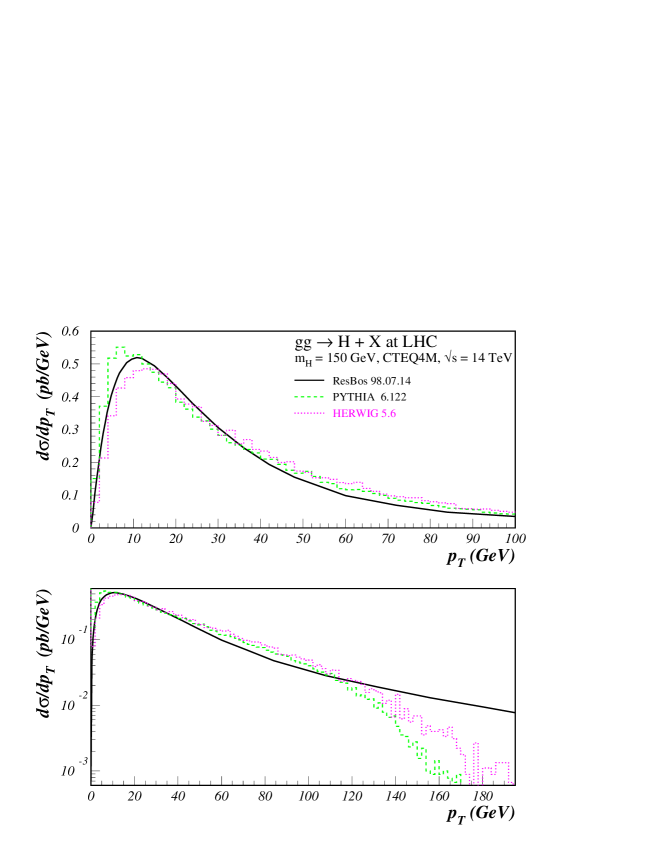
Figure 30: A comparison of predictions for the Higgs $p_{T}$ distribution at the LHC from ResBos, two recent versions of Pythia and Herwig. The ResBos, Pythia and Herwig predictions have been normalized to the same area.

3.4.3 Comparison with Herwig

The variation between versions 5.7 and 6.1 of Pythia gives an indication of the uncertainties due to the types of choices that can be made in Monte Carlos. The requirement that $\hat{u}$ be negative for all branchings is a choice rather than an absolute requirement. Perhaps the better agreement of version 6.1 with ResBos is an indication that the adoption of the $\hat{u}$ restrictions was correct. Of course, there may be other changes to Pythia which would also lead to better agreement with ResBos for this variable.

Since there are a variety of choices that can be made in Monte Carlo implementations, it is instructive to compare the predictions for the $p_{T}$ distribution for Higgs production from ResBos and Pythia with that from Herwig (version 5.6, also using the CTEQ4M parton distribution functions). The Herwig prediction is shown in Figure 30 along with the Pythia and ResBos predictions, all normalized to the ResBos prediction. In all cases, the CTEQ4M parton distribution was used. The predictions from Herwig and Pythia 6.1 are very similar, with the Herwig prediction matching the ResBos shape somewhat better at low $p_{T}$. An understanding of the signature for Higgs boson production at either the Tevatron or LHC depends upon the understanding of the details of soft gluon emission from the initial state partons. This soft gluon emission can be modelled either in a Monte Carlo or in a resummation calculation, with various choices possible in both implementations. A comparison of the two approaches is useful to understand the strengths and weaknesses of each. The data from the Tevatron that either exists now, or will exist in Run 2, will be extremely useful to test both approaches.

In contrast to the case for Z production at the Tevatron, the Higgs cross section at the LHC is not particularly sensitive to the non–perturbative $k_{T}$ added at the scale $Q_{0}$. In the evolution to the hard scatter scale $Q$, the $k_{T}$ is ‘radiated away’, given the enhanced gluon radiation probability present for a $gg$ initial state. For a more thorough discussion of the comparison between analytic methods and parton showers, see Ref. [193].

3.5 CompHEP for LHC

The CompHEP package is available from: http://theory.npi.msu.su/~comphep/. A version adapted to the LHC physics CompHEP V.33 [138], including executable Linux modules is available at CERN from: /afs/cern.ch/cms/physics/COMPHEP-Linux.

The current CompHEP version performs all calculation at tree level (LO). Three issues must be discussed as they open several setting options: a) the parton distributions, b) the QCD scale, and c) the running strong coupling.

In CompHEP v.33, the following parton distribution sets are implemented: MRS(A’) and MRS(G) [200], CTEQ4l and CTEQ4m [111]. Note that CTEQ4l is a LO parametrization, while in all others the evolution of parton distributions is treated at NLO. Dedicated routines are available to allow the addition of any other defined parton distribution (e.g. CTEQ5).

As discussed in Sect. 1, the factorization theorem states that the parton distribution depends not only on Bjorken variable $x$ but also on its virtuality $Q^{2}$ or, equivalently, on the factorization scale. This parameter is related to the energy (or momentum) scale which characterizes the hard subprocess, but it cannot be unambiguously fixed (see Sect. 1). Therefore it can be experimentally tuned. It can be set by the user for each specific QCD process as either fixed or running. In the latter case, $Q^{2}$ can be set to any linear combination squared of the external particles momenta (e.g. $(p_{1}-p_{3})^{2}$, $(p_{1}-p_{3}-p_{4})^{2}$, $(p_{3}+p_{4})^{2}$ …where initial and outgoing momenta enter with opposite signs).

In CompHEP V.33, the QCD coupling $\alpha_{\mathrm{S}}$ can be computed at LO, NLO or NNLO precision. All the corresponding formulas are written in terms of $\Lambda_{\overline{\mbox{\rm{\small{MS}}}}}^{(6)}$, the fundamental QCD scale for $N_{f}=6$ flavours of massless quarks (see Sect. 1 and [13]). In CompHEP, to evaluate a QCD process, one first fixes the $\alpha_{\mathrm{S}}$ normalization point (e.g. a popular normalization point is the mass of $Z$ boson, $Q=M_{Z}$) to which correspond an experimental fit (e.g. $\alpha_{\mathrm{S}}^{NLO}(M_{Z})=0.118$). Then, the corresponding $\Lambda_{\overline{\mbox{\rm{\small{MS}}}}}^{(N_{f})}$ ($N_{f}=5$ at $Q=M_{Z}$) can be deduced from the $\alpha_{\mathrm{S}}$ expression at the selected precision order. The CompHEP input parameter $\Lambda_{\overline{\mbox{\rm{\small{MS}}}}}^{(6)}$ is then obtained from $\Lambda_{\overline{\mbox{\rm{\small{MS}}}}}^{(N_{f})}$. Finally, the choice of the QCD scale $Q$ determines $\alpha_{\mathrm{S}}$ and the factorization scale for the pdf’s. Therefore, complete LO calculations of LHC processes are made available for a consistent phenomenological analysis of the influence of higher order contributions.

3.5.1 CompHEP-Pythia interface

An interface between CompHEP and Pythia can be found in:
/afs/cern.ch/cms/physics/COMPPYTH.

A library of CompHEP based partonic event generators for LHC processes has been initiated and various samples of event are available at: /afs/cern.ch/cms/physics/PEVLIB for $Zb\bar{b}$, $Wb\bar{b}$, $t\bar{t}b\bar{b}$ and some others. Unweighted event sample files, located in the corresponding directories (see the files README for details) when handled by the CompHEP-Pythia interface code, generate complete LHC events, ready to be fed to the detector simulation software. For example, the $Zb\bar{b}$ process can be found in: /afs/cern.ch/cms/physics/PEVLIB/Z_b_b. The file __pevZbb contains about 200K unweighted events. Each event is represented by the Lorentz momenta of all external particles. In the current version of the package, there is no color information associated to the events. Thus, only the Independent Fragmentation Model can be invoked. One can always require the Lund model option for the fragmentation, as long as the corresponding color strings have been set by an external algorithm in the routine PYUPEV. The same remark applies also to the final state radiations (FSR), which are, by default, switched off in CompHEP-Pythia interface although initial state radiations (ISR) are switched on. In the upcoming version of the CompHEP package [201] color strings will be generated from the matrix element factors allowing for the use of the Lund fragmentation model.

3.6 Grace for LHC

The URL of web page for the Grace system is http://www-sc.kek.jp/minami/ where the latest information, the reports and manuals [130, 131], the Grace version.2 and the other products are available.

The automated system allows us to create event generators for complicated processes which are hard to calculate by hand. For instance the process $gg\rightarrow b\bar{b}b\bar{b}$ has been calculated without any approximation (e.g. accounting for massive fermions) by use of the Grace system [130, 131].

The intrinsic function of the Grace system is to generate the amplitude for a specified parton interaction. The system has been tested for many reactions and it was confirmed to be able to manage 2-body to 6-body final state processes. The interface with the pdf’s, PS and the fragmentation tools will be implemented in the coming versions (see for example Grape for $ep\rightarrow\ell\bar{\ell}X$ [202]). For the parton showering and the fragmentation, two kinds of approach can be followed. The first is, like in Grape a 2 step procedure: the Bases/Spring package including pdf’s is used for the integration over the phase space and for the generation of unweighted events. If the “kinematics” code is appropriate, Spring generates events with high efficiency and writes the four-vectors of the final-state particles on a temporary file. Then the generated momenta are passed to Pythia for PS and fragmentation. The other approach is more convenient but more complex. Here the code including the kinematics and the generated matrix element is prepared so that Pythia can drive them directly. This type of interface is tested till now only for the processes whose final state consist of 2-, 3- and 4-bodies.

The Grace system can automatically deal with one-loop processes (NLO) for the electroweak and QED-like QCD interactions. For the final two-body processes the performance has been shown to be good. The application to the multi-body final states, however, would be limited because of the huge CPU time required when the code is used as event generators. For such cases a practical use of the generated code will be to evaluate the cross sections and to give the distribution of several physical quantities rather than providing event generators.

As mentioned the contributions beyond LO are crucial for a detailed QCD study. Since the PS method is based on the renormalization group equation, it works as a bridge between the “hard” parton collision and the fragmentation. This bridge is built on the solid and reliable ground of perturbative QCD. In other words the parton shower provides an unambiguous theoretical understanding of $pp(\overline{p})$ interactions except for the “soft” component which cannot be controlled by the perturbative QCD. However, the PS in LL order is not enough. One of the shortcomings is as follows. The pdf’s for the initial state, products of elaborated works, are parameterized according to the NLO QCD formulas. On the other hand the corresponding PS, implemented in the existing programs like Pythia, is evolved using only the LL algorithm at least in their current status. Then the systematic summation of large logarithms up to NLL order must solve this annoying situations. Though the basic technology has been already established and known for many years [203, 204, 205], its implementation is not a trivial task as simply imagined. First it is process-dependent. Once the idea evolves and is realized as one of the environments of Grace, it should allow more precise prediction for LHC. Thus this must be the biggest issue to us.

3.7 Alpha for LHC

As discussed in the introduction to this Section, the ability to evaluate production rates for multi-jet final states will be fundamental at the LHC to study a large class of processes, within and beyond the SM. As was also discussed in the Sect. 3.1, a necessary feature of any multi-jet calculation is the possibility to properly evolve the purely partonic final state, for which exact fixed-order perturbative calculations can be performed, into the observable hadronic final state. This evolution is best performed using shower Monte Carlo calculations. The accurate description of color-coherence effects, furthermore, requires as noticed in the introduction a careful bookkeeping of the contribution to the matrix elements of all possible color configurations. The goal of the algorithm [137] described in this Section is to allow the effective calculation of multi-parton matrix elements, allowing the separation, to the leading order in $1/N_{c}^{2}$ ($N_{c}=3$ being the number of colors), of the independent color configurations. This technique allows an unweighting of the color configurations, and allows the merging of the parton level calculation with the Herwig Monte Carlo.

The key element of the strategy is the use of the algorithm ALPHA, introduced in Ref. [134] for the evaluation of arbitrary multi-parton matrix elements. This algorithm determines the matrix elements from a (numerical) Legendre transform of the effective action, using a recursive procedure which does not make explicit use of Feynman diagrams. The algorithm has a complexity growing like a power in the number of particles, compared to the factorial-like growth that one expects from naive diagram counting. This is a necessary feature of any attempt to evaluate matrix elements for processes with large numbers of external particles, since the number of Feynman diagrams grows very quickly beyond any reasonable value. For example, this calculation allowed [137] the evaluation of the matrix elements for the production of 8-gluon final states. The number of Feynman diagrams which describe this process exceeds 7 billion.

The interface of the parton level scattering matrix element with the PS requires the capability to reconstruct the appropriate color flow for a given event. The strategy to deal with this issue is described in detail in [137]. The following points have to be noticed:

1. Dual amplitudes [206, 207, 208] can be easily evaluated using the ALPHA algorithm. Since the dual amplitudes $A$ are independent of the number $N_{c}$ of colors, they can be calculated exactly by taking $N_{c}$ sufficiently large.

2. With an appropriate choice for the color of the external partons, the full amplitude is proportional to a single dual amplitude.

We explicitly calculated $n$-gluon dual amplitudes using the large-$N_{c}$ Lagrangian. The correctness of the calculation was checked for $n$ up to 11 by comparing the results for maximally helicity violating (MHV) amplitudes [209] (e.g. $g^{+}g^{+}\rightarrow g^{+}\cdots g^{+}$) with the analytic expressions known exactly for arbitrary $n$ [206, 207, 208, 124]. The input of the numerical evaluation of the matrix element is a string containing the total number of gluons, their helicity state, and their momenta. From these data, the amplitude is evaluated automatically.

The prescription to correctly generate the parton-shower associated to a given event in the large-$N_{c}$ limit is therefore the following:

1. Calculate the $(n-1)!$ dual amplitudes corresponding to all possible planar color configurations.

2. Extract the most likely color configuration for this event on a statistical basis, according to the relative contribution of the single configurations to the total event weight . Since each dual amplitude is gauge invariant, the choice of color-configurations is also a gauge-invariant operation.

3. Develop the PS out of each initial and final-state parton, starting from the selected color configuration. This step can be carried out by feeding the generated event to a Monte-Carlo program such as Herwig, which is precisely designed to turn partons into jets starting from an assigned color-ordered configuration.

Notice that, if the dual amplitudes are evaluated for a specific helicity configuration, Herwig will also include spin-correlation effects in the evolution of the parton shower [210, 211, 171, 116, 117].

As a result, use of the dual-amplitude representation of a multi-gluon amplitude allows to accurately describe not only the large-angle correlations in multi-jet final states, but also the full shower evolution of the initial- and final-state partons with the same accuracy available in Herwig for the description of 2-jet final states.

In alternative to the above prescription, one can use ALPHA to calculate the matrix elements for external states with assigned colors. Since these states are all orthogonal, such an approach is particularly efficient if one wants to use a Monte Carlo approach to the summation over all possible color states. The program will then extract through a standard unweighting (at the leading order in $1/N_{c}^{2}$) a specific color flow from all possible color flows contributing to a given orthogonal color state. This color flow is then suitable as an initial condition for the shower evolution. Further details can be found in [137]. At this time, the program is only available in its parton-level form, and allows the calculation of matrix elements for $gg\rightarrow g\dots g$ and $q\overline{q}\rightarrow g\dots g$ processes, with up to 8 final-state gluons. A full version including the interface with Herwig is being prepared.

4 AVAILABLE NLO CALCULATIONS AND PROSPECTS AT NNLO

4.1 Available NLO calculations of multijet processes

QCD calculations of multijet processes beyond LO in the strong coupling constant $\alpha_{\mathrm{S}}$ are quite involved. Nowadays we know (see below) how to perform in general calculations of the NLO corrections to multijet processes, and almost every process of interest has been computed to that accuracy. Instead, the calculation of the NNLO corrections is still at an organisational stage and represents a main challenge. Why should we perform calculations which are technically so complicated ?

The general motivation is that the calculation of the NLO corrections allows us to estimate reliably a given production rate, while the NNLO corrections allow us to estimate the theoretical uncertainty on the production rate. That comes about because higher-order corrections reduce the dependence of the cross section on the renormalization scale, $\mu_{R}$, and for processes with strongly-interacting incoming particles the dependence on the factorization scale, $\mu_{F}$, as well.

An example is the determination of $\alpha_{\mathrm{S}}$ from event shape variables in $e^{+}e^{-}\rightarrow 3$ jets [212, 213, 214, 215]. The calculation of the NNLO contributions to this process would be needed to further reduce the theoretical uncertainty in the determination of $\alpha_{\mathrm{S}}$. An additional motivation for performing calculations at NNLO is to obtain a more accurate theoretical determination of signal and QCD background to Higgs production (for further details, see Sect. 9).

In recent years it has become clear how to construct general-purpose algorithms for the calculation of multijet processes at NLO accuracy. The crucial point is to organise the cancellation of the infrared (i.e. collinear and soft) singularities of the QCD amplitudes in a universal, i.e. process- and observable-independent, way. The universal terms in a NLO calculation are given by the tree-level collinear [14, 216, 16, 17] and soft [217, 218, 219] functions, and by the universal structure of the poles of the one-loop amplitudes [160, 220, 221]. The universal NLO terms and the process-dependent amplitudes are combined into effective matrix elements, which are devoid of singularities. The various NLO algorithms (phase-space slicing [160, 222, 223, 224] and subtraction method [161, 225, 227, 226, 162]) provide different methods to construct the effective matrix elements. These can be integrated in four dimensions, in practice almost always numerically, due to the complexity of the integrand. The integration can be performed with arbitrary experimental acceptance cuts.

We now outline how to perform a NLO calculation of a generic physical observable. As is well known from Bloch-Nordsieck and Kinoshita-Lee-Nauenberg theorems, QCD (like QED) does not have an infinite-resolution power; any attempt to compute the kinematical properties of a fixed number of final-state quarks and gluons results in an infrared-divergent cross section. In order to obtain finite quantities, all the partonic subprocesses which contribute to the same order in $\alpha_{\mathrm{S}}$ to the squared amplitude have to be included in the computation, regardless of the number of final-state particles. In addition, one is forced to consider variables which are inclusive enough to be infrared safe. Roughly speaking, an observable is said to be infrared safe when its value, computed with the kinematical variables of the final-state partons, does not change abruptly when a soft gluon is emitted, or a parton splits almost collinearly into a pair of partons. More technically, an infrared-safe observable must have a smooth limit (that is, must behave continuously) in the following three configurations: a) when a gluon in the final state gets soft; b) when two partons in the final state tend to get collinear to each other; c) when an initial-state parton emits collinearly another parton.

At NLO (assuming that the LO cross section gets contributions from the $n$-parton amplitudes), this implies that one has simply to consider two contributions, denoted as virtual and real. The former is the product of the $n$-parton one-loop amplitudes with the $n$-parton tree amplitudes, while the latter is the square of the $(n+1)$-parton tree amplitudes. In order to deal with finite quantities in the intermediate steps of the calculation, we adopt dimensional regularization – i.e. we change the dimensionality of space-time to $d=4-2\epsilon$. Thus, we can schematically write the virtual and real contributions to the cross section as follows:

$$\left(\frac{d\sigma}{dx}\right)_{\scriptscriptstyle V}=\frac{1}{2\epsilon}\,\delta(1-x)\,,\qquad\qquad\left(\frac{d\sigma}{dx}\right)_{\scriptscriptstyle R}=\frac{1}{1-x}\,;$$ (25)

here, $1-x$ represents the radiated energy. So, $x=1$ means no radiation, and $x=0$ is the maximum of radiation. The relevant physical quantity will be the average value $<F>$ of a certain function $F(x)$; for example, we can think of $F$ as being the product of theta functions representing a histogram bin. Then, the NLO contribution to $<F>$ is

$$<F>_{\scriptscriptstyle\rm NLO} = \int_{0}^{1}dx\,\left(\frac{d\sigma}{dx}\right)_{\scriptscriptstyle V}\!F(x)+\int_{0}^{1}dx\,(1-x)^{-2\epsilon}\,\left(\frac{d\sigma}{dx}\right)_{\scriptscriptstyle R}\!F(x)$$ (26)

$$= \frac{1}{2\epsilon}\int_{0}^{1}dx\,\delta(1-x)\,F(x)+\int_{0}^{1}dx\,(1-x)^{-1-2\epsilon}\,F(x)$$ (27)

$$= \frac{1}{2\epsilon}\,F(1)+<F>_{\scriptscriptstyle R}\,.$$ (28)

The factor $(1-x)^{-2\epsilon}$ in the real contribution comes from the necessity of performing the computation in $d$ dimensions, in order to regulate the divergences arising when performing the integration over the phase space. As it is apparent from eq. (27), the most difficult task is the computation of the real contribution. In practice, the form of $F(x)$ is too complicated to perform an analytical integration. On the other hand, we cannot proceed straightforwardly, and compute the integral numerically; in fact, the integral is divergent in the limit $\epsilon\rightarrow 0$, and the pole in $1/\epsilon$ will exactly cancel that explicitly displayed in the virtual contribution (provided that $F$ describes an infrared-safe quantity).

Two strategies have been developed to tackle this problem. In the framework of the slicing method, the real contribution is rewritten as follows:

$$<F>_{\scriptscriptstyle R}=\int_{0}^{1-\delta}dx\,\frac{F(x)}{(1-x)^{1+2\epsilon}}+\int_{1-\delta}^{1}dx\,\frac{F(x)}{(1-x)^{1+2\epsilon}},$$ (29)

where $\delta$ is an arbitrary parameter, $0<\delta\leq 1$. The first term on the right hand side of this equation is free of divergences ($F(x)$ is regular in the limit $x\rightarrow 1$); in this term, one can therefore set $\epsilon=0$, and compute the integral with standard numerical methods. On the other hand, the second term is still divergent for $\epsilon\rightarrow 0$; however, if $\delta$ is small enough, one can approximate $F(x)$ with $F(1)$ (that is, with the first term of its Taylor expansion around $x=1$). Therefore

$$<F>_{\scriptscriptstyle R} = \int_{0}^{1-\delta}dx\,\frac{F(x)}{1-x}+F(1)\int_{1-\delta}^{1}dx\,\frac{1}{(1-x)^{1+2\epsilon}}+{\cal O}(\delta)$$ (30)

$$= \int_{0}^{1-\delta}dx\,\frac{F(x)}{1-x}-\frac{\delta^{-2\epsilon}}{2\epsilon}F(1)+{\cal O}(\delta)\,.$$ (31)

Eq. (31) can now be substituted into eq. (28). Expanding eq. (31) in powers of $\epsilon$, keeping only the terms which do not vanish in the limit $\epsilon\rightarrow 0$, and neglecting the contributions of the terms of ${\cal O}(\delta)$, we see that the pole terms in $1/\epsilon$ cancel, and one is left with a finite result:

$$<F>_{\scriptscriptstyle\rm NLO}^{slicing}=\int_{0}^{1-\delta}dx\,\frac{F(x)}{1-x}+F(1)\log\delta.$$ (32)

At a first glance, this expression is seemingly puzzling: the parameter $\delta$ is arbitrary, and the physical results should not depend on it. However, it is easy to see that the upper bound of the integral gives a contribution behaving (approximately) like $-F(1)\log\delta$. It has to be stressed that the slicing method is based on the approximation performed in eq. (30); for this approximation to hold, it is crucial that $\delta$ is as small as possible; otherwise, the terms collectively denoted with ${\cal O}(\delta)$ in eq. (31) are not negligible. On the other hand, in practical computations, the integral in eq. (32) is performed numerically; due to the divergence of the integrand for $x\rightarrow 1$, $\delta$ cannot be taken too small, because of the loss of accuracy of the numerical integration. Thus, the value of $\delta$ is a compromise between these two opposite requirements, being neither too small nor too large. Of course, “small” and “large” are meaningful only when referred to a specific computation. Therefore, when using the slicing method, it is mandatory to check that the physical results are stable against the variation of the value of $\delta$, chosen in a suitable range. In principle, this check would have to be performed for each observable $F$ computed; in practice, only one observable is checked, generally chosen to be rather inclusive (such as a total rate).

Another possibility to compute $<F>_{\scriptscriptstyle R}$ is given by the subtraction method. One writes

$$<F>_{\scriptscriptstyle R}=\int_{0}^{1}dx\,\frac{F(x)-F(1)\theta(x-1+x_{c})}{(1-x)^{1+2\epsilon}}+F(1)\int_{0}^{1}dx\,\frac{\theta(x-1+x_{c})}{(1-x)^{1+2\epsilon}},$$ (33)

where $x_{c}$ is an arbitrary parameter $0<x_{c}\leq 1$. The first term on the right hand side of this equation is convergent, and we can set $\epsilon=0$. The second term is formally identical to the one appearing in eq. (30). Notice, however, that no approximation has been made in eq. (33); the price to pay is a more complicated expression for the first integral. Proceeding as before, we get:

$$<F>_{\scriptscriptstyle\rm NLO}^{subt}=\int_{0}^{1}dx\,\frac{F(x)-F(1)\theta(x-1+x_{c})}{1-x}+F(1)\log x_{c}.$$ (34)

This equation has to be compared to eq. (32); although the two are quite similar, there are two important differences that have to be stressed. Firstly, the parameter $x_{c}$ introduced in the subtraction method does not need to be small (actually, in the original formulation of the method $x_{c}$ was not even introduced, which corresponds to set $x_{c}=1$ here). This is due to the fact that in the subtraction method no approximation has been performed in the intermediate steps of the computation. This in turn implies the second point: there is no need to check that the physical results are independent of the value of $x_{c}$, since this is true by construction.

The universal algorithms previously mentioned allow the computation of any infrared-safe observable in a straightforward manner; the matrix elements do not need any algebraic manipulation, and can be computed in four dimensions. It is therefore relatively easy to construct computer codes, accurate to NLO in QCD, that are flexible enough to become a useful tool in the analysis of the experimental data. In the following, we will list the codes which are of direct interest for the physics of high-energy hadronic collisions. We do not intend to give a complete list of references to the papers relevant for the calculation of a given production process , but rather only to quote the computer codes which will have a chance to be used by the experimental collaborations at the LHC. Most of the codes listed here are available as free software.

• Jets

  • S.D. Ellis, Z. Kunszt and D.E. Soper [220, 6], subtraction, computes one- and two-jet observables.

  • W.T. Giele, E.W.N. Glover and D.A. Kosower (JETRAD) [222], slicing, computes one- and two-jet observables.

  • S. Frixione [227], subtraction, computes one- and two-jet observables.

  • W. Kilgore and W.T. Giele [228], slicing, computes three-jet observables.

• Single Isolated Photon (plus one jet)

  • H. Baer, J. Ohnemus and J.F. Owens [229], slicing, fragmentation contribution computed to LO accuracy.

  • L.E. Gordon and W. Vogelsang [230], analytical integration over the variables of the recoiling partons: no information on the accompanying jet; dependence on the isolation variables treated to logarithmic approximation.

  • S. Frixione [231], subtraction, only effective with the isolation prescription of ref. [232].

  • M. Werlen (PHONLL) [http://home.cern.ch/~monicaw/phonll.html], slicing, based on ref. [234, 233].

• Isolated-Photon Pairs

  • B. Bailey, J.F. Owens and J. Ohnemus [235], slicing, fragmentation contributions computed to LO accuracy.

  • C. Balazs, E.L. Berger, S. Mrenna and C.P. Yuan [236], slicing, resummation effects included, fragmentation contributions computed with parton shower methods.

  • T.Binoth, J.Ph. Guillet, E. Pilon and M.Werlen (DIPHOX) [237], slicing, all contributions computed to NLO accuracy.

• Single Heavy Vector Boson (plus one jet)

  • W.T. Giele, E.W.N. Glover and D.A. Kosower (DYRAD) [222], slicing.

• Single Heavy Vector Boson plus one photon

  • U. Baur, T. Han, J. Ohnemus [238, 239], slicing.

  • D. de Florian and A. Signer [240], subtraction, includes spin correlations in the decay of the bosons; fragmentation contributions computed to LO accuracy.

• Heavy Vector Boson Pairs

  • U. Baur, T. Han, J. Ohnemus and J.F. Owens [241, 242, 243, 244, 245], slicing.

  • S. Frixione, B. Mele, P. Nason and G. Ridolfi [246, 247, 248], subtraction.

  • J.M. Campbell and R.K. Ellis (MCFM) [249], subtraction, includes spin correlations in the decay of the bosons.

  • L. Dixon, Z. Kunszt and A. Signer [250], subtraction, includes spin correlations in the decay of the bosons.

• Higgs Boson at large transverse momentum (plus one jet)

  • D. de Florian and M. Grazzini and Z. Kunszt [197], subtraction, computes Higgs-boson production in the infinite top-quark-mass limit.

• Heavy Quarks

  • M. Mangano, P. Nason and G. Ridolfi [251], subtraction, computes single-inclusive distribution and correlations betweeen $Q$ and $\overline{Q}$.

Since the universal algorithms accomplish the task of cancelling the infrared divergences of the virtual and real contributions in a process-independent way, the remaining work that has to be performed to calculate a production rate at NLO is the computation of the appropriate tree and one-loop amplitudes. As we said previously, to compute $n$-jet production at NLO, two sets of amplitudes are required: a) $n$-particle production amplitudes at tree level and one loop; b) $(n+1)$-particle production amplitudes at tree level. If the one-loop amplitudes are regularised through dimensional regularisation, it suffices at NLO to compute them to ${\cal O}(\epsilon^{0})$.

Efficient methods based on the color decomposition [125, 252, 253, 254] of an amplitude in color-ordered subamplitudes, which are then projected onto the helicity states of the external partons, have largely enhanced the ability of computing tree [125] and one-loop [255] amplitudes. Accordingly, tree amplitudes with up to seven massless partons [125, 256, 257] and with a vector boson and up to five massless partons [258] have been computed analytically. In addition, efficient techniques to evaluate numerically tree multi-parton amplitudes have been introduced [259, 137] (see Sect. 3 for a description of available numerical codes), and have been used to compute tree amplitudes with up to eleven massless partons [137]. The calculation of one-loop amplitudes can be reduced to the calculation of one-loop $n$-point scalar integrals [260, 261, 262]. The reduction method [260] allowed the computation of one-loop amplitudes with four massless partons [263] and with a vector boson and three massless partons [264]. However, one-loop scalar integrals present infrared divergences, induced by the massless external legs. For one-loop multi-parton amplitudes, the infrared divergences hinder the reduction methods of ref. [260, 261, 262]. This problem has been overcome in ref. [265, 266]. Accordingly, one-loop amplitudes with five massless partons [267, 269, 268] and with a vector boson and four massless partons [270, 271, 272, 273, 274] have been computed analytically. The reduction procedure of ref. [265, 266] has been generalised in ref. [275], where it has been shown that any one-loop $n$-point scalar integral, with $n>4$, can be reduced to box scalar integrals. The calculation of one-loop multi-parton amplitudes thus can be pushed a step further in the near future.

4.2 Prospects for NNLO calculations

Eventually, a procedure similar to the one followed at NLO will permit the construction of general-purpose algorithms at NNLO accuracy. It is mandatory then to fully investigate the infrared structure of the matrix elements at NNLO. The universal pieces needed to organise the cancellation of the infrared singularities are given by the tree-level triple-collinear [276, 277, 253], double-soft [219, 278] and soft-collinear [276, 278] functions, by the one-loop splitting [271, 279, 280, 281] and eikonal [271] functions, and by the universal structure of the poles of the two-loop amplitudes [282]. These universal pieces have yet to be assembled together, to show the cancellation of the infrared divergences at NNLO.

Then to compute $n$-jet production at NNLO, three sets of amplitudes are required: a) $n$-particle production amplitudes at tree level, one loop and two loops; b) $(n+1)$-particle production amplitudes at tree level and one loop; c) $(n+2)$-particle production amplitudes at tree level. In dimensional regularisation at NNLO, the two-loop amplitudes need be computed to ${\cal O}(\epsilon^{0})$, while the one-loop amplitudes must be evaluated to ${\cal O}(\epsilon^{2})$ [271, 283]. The main challenge is the calculation of the two-loop amplitudes. At present, the only amplitude known at two loops is the one for $V\leftrightarrow q\overline{q}$ [284, 285, 32], with $V$ a massive vector boson, which depends only on one kinematic variable. It has been used to evaluate the NNLO corrections to Drell-Yan production [32, 33] and to deeply inelastic scattering (DIS) [64, 63]. Two-loop computations for configurations involving two kinematic variables, which are needed in the case of parton-parton scattering, exist only in the special cases of maximal supersymmetry [286], and of maximal helicity violation [287]. The latter contributes only beyond NNLO. One of the main obstacles for configurations involving two kinematic variables is the analytic computation of the two-loop four-point functions with massless external legs, where significant progress has just been achieved. These consist of planar double-box integrals [288, 289], non-planar double-box integrals [290], single-box integrals with a bubble insertion on one of the propagators [291] and single-box integrals with a vertex correction [292]. Finally, processes such as $e^{+}e^{-}\rightarrow 3\,jets$ and $p\,p\rightarrow H\,jet$ sport configurations involving three kinematic variables and require the analytic computation of two-loop four-point functions with a massive external leg. Some of the required two-loop four-point functions of this kind have been derived recently [293]. Another obstacle is the color decomposition of two-loop amplitudes, which is not generally known yet. Substantial progress is expected in the near future on all the issues outlined above, which should make the present note soon outdated.

Finally, we mention that in the factorization of collinear singularities for strongly-interacting incoming particles, the evolution of the pdf’s in the jet cross section should be determined to an accuracy matching the one of the parton cross section. For hadroproduction of jets computed at NLO, one needs the NLO AP splitting functions for the evolution of the pdf’s (see Eqs. (8) and (9)). Accordingly, for hadroproduction at NNLO the evolution of the pdf’s should be computed using the NNLO AP splitting functions. Except for the lowest five (four) even-integer moments of the NNLO non-singlet (singlet) AP splitting functions [25, 26], no calculation of the NNLO evolution of the pdf’s exists yet. Some NNLO analyses based on the finite set of known moments have been performed for the DIS structure functions $xF_{3}$ and $F_{2}$ (see Sects. 2.5 and 2.6 and Ref. [99]). Furthermore, in ref. [70] a quantitative assessment of the importance of the yet unknown higher-order terms has been performed, with the conclusion that they should be numerically significant only for Bjorken $x$ smaller than $10^{-2}$.

The computation of the evolution kernels of the pdf’s at NNLO accuracy is a major challenge in QCD. The NLO computation was performed with two different methods, one using the operator product expansion (OPE) in a covariant gauge [18, 19, 20, 21, 24], the other using the light-cone axial (LCA) gauge with principal value prescription  [22, 23]. However, the prescription used in ref. [22, 23] has certain shortcomings. Accordingly, the calculation has been repeated in the LCA gauge using a prescription [294, 295] which makes it amenable to extensions beyond NLO, whereas the principal value prescription does not seem to be applicable beyond NLO [296]. On the other hand, using the OPE method, there had been a problem with operator mixing in the singlet sector, which has been fixed [297, 298, 299] only recently, and the result finally coincides with the one obtained in the LCA gauge in ref. [23]. Thus the result for the AP splitting functions at NLO accuracy is fully under control. Recent proposals for their calculation beyond NLO include extensions of the OPE technique, which have been used to recompute the NNLO corrections to DIS [300], and a computation based on combining universal gauge-invariant collinear pieces [301].

5 SUMMATIONS OF PERTURBATION THEORY

5.1 Summations of logarithmically-enhanced contributions

The calculation of hard–scattering cross sections in hadron collisions requires the knowledge of partonic cross sections ${\hat{\sigma}}$, as well as that of parton densities (see the factorization formula in Eq. (2)). The partonic cross sections ${\hat{\sigma}}(p_{1},p_{2};Q,\{Q_{1},\dots\};\mu^{2})$ are usually computed by truncating their perturbative expansion at a fixed order in $\alpha_{\mathrm{S}}$, as in Eq. (3). However, fixed–order calculations are quantitatively reliable only when all the kinematical scales $Q,\{Q_{1},\dots\}$ are of the same order of magnitude. When the hard–scattering process involves two (or several) very different scales, say $Q\gg Q_{1}$, the $n$-th term in Eq. (3) can contain double– and single–logarithmic contributions of the type $(\alpha_{\mathrm{S}}L^{2})^{n}$ and $(\alpha_{\mathrm{S}}L)^{n}$ with $L=\ln(Q/Q_{1})\gg 1$. These terms spoil the reliability of the fixed–order expansion and have to be summed to all orders, systematically improving on the logarithmic accuracy of the expansion.

Typical examples of such large logarithms are the terms $L=\ln Q/Q_{0}$ related to the evolution of parton densities (and parton fragmentation functions) from a low input scale $Q_{0}$ to the hard–scattering scale $Q$. These logarithms are produced by collinear radiation from the colliding partons and give single–logarithmic contributions. They never explicitly appear in the calculation of the partonic cross section, because they are systematically (LO, NLO and so forth) resummed in the evolved parton densities $f_{a/h}(x,Q^{2})$ and parton fragmentation functions $d_{a/H}(x,Q^{2})$ by using DGLAP equations (8).

A different sort of large logarithm, $L=\ln{\sqrt{s}}/Q$, arises when the centre–of–mass energy ${\sqrt{s}}$ of the collision is much larger than the hard scale $Q$. These small–$x$ $(x=Q/{\sqrt{s}})$ logarithms are produced by multiple gluon radiation over the wide rapidity range that is available at large energy. For sufficiently inclusive processes in singlet channels these give single–logarithmic (LLx) contributions that can be calculated by using the BFKL equation [302, 303, 304, 305, 306]. The subleading (NLLx) contributions have also been calculated recently [67, 307] and turn out to be very large. This is understood to be due to contamination by collinear logarithms of $Q^{2}/Q_{0}^{2}$, which must be simultaneously resummed to obtain reliable predictions at small $x$ [308, 309]. Various resummation procedures have been suggested, and will be briefly discussed in Sects. 5.4 and 7 Unfortunately there are as yet no substantial phenomenological analyses which use these resummations. The resummation of small–$x$ logarithms will be important for the accurate determination of the behaviour of singlet parton densities $f_{a/h}(x,Q^{2})$ at small values of the parton momentum fraction $x$, and thus for making reliable predictions of any process that is sensitive to the hard–scattering of low–momentum partons (for example $b$–quark production and inclusive production of low–$E_{T}$ jets and prompt photons at the LHC). The BFKL equation is however also relevant for understanding the structure of final states, for example when there are jets with large rapidity intervals, or diffractive processes with large rapidity gaps. These more general aspects of small–$x$ physics are discussed in Sect. 7

Yet another class of large logarithms is associated to the bremsstrahlung spectrum of soft gluons. Since soft gluons can be radiated collinearly, they give rise to double–logarithmic contributions to the partonic cross section, which takes the form

$${\hat{\sigma}}\sim\alpha_{\mathrm{S}}^{k}~{}{\hat{\sigma}}^{(LO)}\left\{1+\sum_{n=1}^{\infty}\alpha_{\mathrm{S}}^{n}\left(C_{2n}^{(n)}L^{2n}+C_{2n-1}^{(n)}L^{2n-1}+C_{2n-2}^{(n)}L^{2n-2}+\dots\right)\right\}\;\;.$$ (35)

Double–logarithmic terms due to soft gluons arise in all the kinematic configurations where the contributions of real and virtual partons are highly unbalanced (see Ref. [218] and references therein).

When partons (particles or jets) with low momentum fraction $z$ are directly triggered in the final state, the rôle of (real) soft radiation is evidently enhanced. The low–momentum region of the fragmentation spectra of particles and subjets in jet final–states is thus particularly sensitive to the resummation of small–$z$ logarithms. The calculations based on the resummation of these logarithms are probably the perturbative predictions that are most sensitive to the coherence properties [218, 310] of QCD. Detailed studies of fragmentation processes have been performed in $e^{+}e^{-}$ annihilation, DIS and at the Tevatron (see the recent review in Ref. [311]). Although this topic is not included in these proceedings, similar studies at the LHC would certainly be valuable.

In different kinematic configurations, (real) radiation in the final state can instead be strongly inhibited. For instance, this happens in the case of transverse momentum distributions at low transverse momentum, in the case of hard–scattering production near threshold or when the structure of the final state is investigated with high resolution (internal jet structure, shape variables).

Soft–gluon resummation for jet shapes has extensively been studied and applied to hadronic final states produced by $e^{+}e^{-}$ annihilation [312, 214, 313]. Applications to hadron–hadron collisions have just begun to appear [314, 315, 316] and have a large, yet uncovered, potential (from $\alpha_{\mathrm{S}}$ determinations to studies of non–perturbative dynamics). Future studies of this topic are certainly warranted.

Threshold logarithms, $L=\ln(1-x)$, occur when the tagged final state produced by the hard scattering is forced to carry a very large fraction $x$ ($x\rightarrow 1$) of the available centre–of–mass energy $\sqrt{s}$. Outstanding examples of hard processes near threshold are DIS at large $x$ (here $x$ is the Bjorken variable), production of DY lepton pairs or di-jets with large total invariant mass $Q=M_{ll}$ or $M_{jj}$ ($x=Q/{\sqrt{s}}$), production of $W$, $Z$ and Higgs bosons ($x=M_{W,Z,H}/{\sqrt{s}}$), production of heavy quark–anti-quark pairs ($x=2m_{Q}/{\sqrt{s}}$), inclusive production of single jets and single photons at large transverse energy $E_{T}$ ($x=2E_{T}/{\sqrt{s}}$).

Transverse–momentum logarithms, $L=\ln Q^{2}/{\bf p}_{T}^{2}$, occur in the distribution of transverse momentum ${{\mbox{\boldmath$p$}}}_{T}$ of systems with high mass $Q$ $(Q\gg p_{T})$ that are produced with a vanishing ${{\mbox{\boldmath$p$}}}_{T}$ in the LO subprocess. Examples of such systems are DY lepton pairs, lepton pairs produced by $W$ and $Z$ decay, heavy quark–anti-quark pairs, photon pairs and Higgs bosons.

Studies of soft–gluon resummation for transverse–momentum distributions at low transverse momentum and hard–scattering production near threshold were pioneered two decades ago [317, 318, 319, 320, 321, 322, 323, 324, 325, 326, 327]. The physical bases for a systematic all–order summation of the soft–gluon contributions are dynamics and kinematics factorizations [328, 329]. The first factorization follows from gauge invariance and unitarity: in the soft limit multigluon amplitudes fulfil factorization formulae given in terms of universal (process independent) soft contributions. The second factorization regards kinematics and strongly depends on the actual cross section to be evaluated. When phase–space kinematics is factorizable, resummation is analytically feasible in the form of a generalized exponentiation of the universal soft contributions that appear in the factorization formulae of QCD amplitudes.

Typically, phase–space factorization does not occur in the space of the kinematic variables where the cross section is defined. It is thus necessary to introduce a conjugate space to overcome phase space constraints. This is the case for hard–scattering production near threshold, where the relevant kinematical constraint is (one–dimensional) energy conservation, which can be factorized performing a Laplace (or Mellin) transformation (see Sect. 5.2). Analogously, the relevant kinematical constraint for ${{\mbox{\boldmath$p$}}}_{T}$–distributions is (two–dimensional) transverse–momentum conservation and it can be factorized by performing a Fourier transformation (see Sect. 5.3). In the conjugate space, the logarithms $L$ of the relevant ratio of momentum scales are replaced by logarithms $\tilde{L}$ of the conjugate variable.

The resummed cross section is thus typically of the form

$${\hat{\sigma}}_{\rm res.}=\alpha_{\mathrm{S}}^{k}\;\int_{\rm inv.}{\hat{\sigma}}^{(LO)}\cdot C\cdot S\;,$$ (36)

where the integral $\int_{\rm inv.}$ denotes the inverse transformation from the conjugate space where resummation is actually carried out. The factor $C$ contains all constant contributions in the limit ${\tilde{L}}\rightarrow\infty$. The singular dependence on ${\tilde{L}}$ is entirely exponentiated in the effective form factor $S$:

$$S=\exp\left\{{\tilde{L}}\;g_{1}(\alpha_{\mathrm{S}}(\mu){\tilde{L}})+g_{2}(\alpha_{\mathrm{S}}(\mu){\tilde{L}};\mu^{2})+\alpha_{\mathrm{S}}(\mu)\;g_{3}(\alpha_{\mathrm{S}}(\mu){\tilde{L}};\mu^{2})+\dots\right\}\;\;.$$ (37)

The structure of the exponent is formally analogous to that of the fixed–order expansion of the partonic cross sections (see Eq. (3)). The function $L\,g_{1}$ resums all the leading logarithmic (LL) contributions $\alpha_{\mathrm{S}}^{n}L^{n+1}$, while $g_{2}$ contains the next–to–leading logarithmic (NLL) terms $\alpha_{\mathrm{S}}^{n}L^{n}$ and so forth. Note that the NLL terms are formally suppressed by a power of $\alpha_{\mathrm{S}}$ with respect to the LL ones, and the same is true for the successive classes of logarithmic terms. Thus, this logarithmic expansion is as systematic as the fixed–order expansion in Eq. (3).

In general, a resummed expression such as Eq. (36) must be properly combined with the best available fixed–order result. Using a shorthand notation, this is achieved by writing the partonic cross section ${\hat{\sigma}}$ as

$${\hat{\sigma}}={\hat{\sigma}}_{\rm res.}+{\hat{\sigma}}_{\rm rem.}\;.$$ (38)

The term ${\hat{\sigma}}_{\rm res.}$ embodies the all–order resummation, while the remainder ${\hat{\sigma}}_{\rm rem.}$ contains no large logarithmic contributions. The latter has the form

$${\hat{\sigma}}_{\rm rem.}={\hat{\sigma}}^{({\rm f.o.})}-\left[\,{\hat{\sigma}}_{\rm res.}\,\right]^{({\rm f.o.})}\;\;,$$ (39)

and it is obtained from ${\hat{\sigma}}^{({\rm f.o.})}$, the truncation of the perturbative expansion for ${\hat{\sigma}}$ at a given fixed order (LO, NLO, …), by subtracting the corresponding truncation $\left[{\hat{\sigma}}_{\rm res.}\right]^{({\rm f.o.})}$ of the resummed part. Thus, the expression on the right–hand side of Eq. (38) includes soft–gluon logarithms to all orders and it is matched to the exact (with no logarithmic approximation) fixed–order calculation. It represents an improved perturbative calculation that is everywhere as good as the fixed–order result, and much better in the kinematics regions where the soft–gluon logarithms become large ($\alpha_{\mathrm{S}}L\sim 1$). Eventually, when $\alpha_{\mathrm{S}}L\mathrel{\hbox to0.0pt{\lower 4.0pt\hbox{\hskip 1.0pt$\sim$}\hss}\raise 1.0pt\hbox{$>$}}1$, the resummed perturbative contributions are of the same size as the non–perturbative contributions and the effect of the latter has to be implemented in the resummed calculation.

Using a matched NLL+NLO calculation as described above, we can consistently introduce a precise definition (say $\overline{\mbox{\rm{\small{MS}}}}$) of $\alpha_{\mathrm{S}}(\mu)$ and investigate the theoretical accuracy of the calculation by studying its dependence on the renormalization/factorization scale $\mu$.

Resummed calculations for hadron collisions near threshold and for $p_{T}$–distributions are discussed in Sects. 5.2 and 5.3, respectively. Some overviews can also be found in Ref. [196]. We refer the reader to Sects. 3.3 and 3.4 for comparisons of resummed calculations with parton shower event generators.

5.2 Threshold resummations

Large logarithms arise in any inclusive cross section for the production of an object with a large mass $Q$, whenever the partonic energy $\sqrt{\hat{s}}$ available for the process is close to $Q$, the production threshold. The physical mechanism responsible for these logarithms is simple. Close to threshold the phase space for the emission of gluon radiation in the final state is kinematically restricted; soft real radiation is, however, responsible for the cancellation of infrared divergences associated with virtual gluon exchange; whenever radiation is inhibited, the cancellation is partially spoiled: finite but large contributions are left over, in the form of logarithms of the ratio of the two relevant energy scales, $\ln[(\hat{s}-Q^{2})/\hat{s}]$. Close to partonic threshold these logarithms become large and must be resummed. Processes for which this resummation is relevant are ubiquitous, as noted in the previous subsection. Techniques to perform threshold resummations have been developed and progressively extended for well over a decade; references in which these techniques are explained is some detail include [330, 331, 332, 333, 334, 335, 336, 337]; here we will briefly review the basic theoretical issues, and sketch the status of phenomenological applications of relevance to the LHC.

As described in the introduction to the present Section, the resummation of threshold logarithms in performed in Mellin space. To illustrate the structure of a typical resummation of threshold logarithms, let us concentrate on the simplest and best known example: the DY cross section. In this case the resummed formula for the Mellin transform of the partonic cross section, in the DIS factorization scheme, takes the form [330, 331]

$$\hat{\sigma}_{{\rm res.}}(N,Q^{2})=C(\alpha_{\mathrm{S}}(Q^{2}))\exp\left[E(N,Q^{2})\right]~{}~{},$$ (40)

where the function $C$ collects terms independent of the Mellin variable $N$, while the exponent can be written as

$$E(N,Q^{2})=-~{}2~{}\int_{0}^{1}dz~{}\frac{z^{N}-1}{1-z}\left[B(\alpha_{\mathrm{S}}((1-z)Q^{2}))+\int_{(1-z)^{2}Q^{2}}^{(1-z)Q^{2}}\frac{dq^{2}}{q^{2}}A(\alpha_{\mathrm{S}}(q^{2}))\right]~{}~{}.$$ (41)

Equations (40) and (41) resum, in principle, all logarithms of $N$ to all orders in perturbation theory, in the sense that all such logarithms exponentiate and are calculable from the functions $A$ and $B$, for which Feynman rules can be derived. In practice, the functions $A$ and $B$ are known only to two loops, so that the resummation can explicitly be performed only for leading and next–to–leading logarithms in the exponent. Performing the integrals in $E(N,Q^{2})$, after expansion of the running couplings in terms of $\alpha_{\mathrm{S}}(Q^{2})$ to the desired accuracy, yields in general an expression of the form

$$E(N,Q^{2})=\ln N~{}g_{1}(\alpha_{\mathrm{S}}\ln N)+g_{2}(\alpha_{\mathrm{S}}\ln N)+\sum_{k=1}^{\infty}\alpha_{\mathrm{S}}^{k}~{}g_{k+2}(\alpha_{\mathrm{S}}\ln N)~{}~{},$$ (42)

where the functions $g_{1}$ and $g_{2}$ are known in terms of the coefficients $A^{(1)}$, $A^{(2)}$ and $B^{(1)}$ of the perturbative expansion of the functions $A$ and $B$, together with the one– and two–loop coefficients of the QCD $\beta$ function. The (unknown) function $g_{3}$, giving the NNL logarithms, would require the determination of $A^{(3)}$, as well as $B^{(2)}$ and the three–loop $\beta$ function.

Several comments are necessary in order to introduce the practical applications of resummed formulas such as Eq. (41).

• At the present level of accuracy (NLL) the dependence on the renormalization scale and on the factorization scheme is under control. A change in renormalization scale shifts the function $g_{2}$ by an amount proportional to the derivative of the function $g_{1}$. A change in factorization scheme changes both $g_{1}$ and $g_{2}$, because it affects the way in which the DIS process is subtracted from DY to construct a finite cross section, however the change is well understood and both functions can be translated from one scheme to another [172, 335].

• To understand the effects of resummation, one should keep in mind that it is performed at the level of the partonic cross section. One consequence of this fact is that resummation generically enhances the cross section, although one might expect a Sudakov suppression, since the probability of having a nearly radiation-less hard scattering is exponentially suppressed. This is easily understood in the DIS scheme: there one computes the (factorized) partonic DY cross section by taking the ratio of the DY process to the square of the DIS process, since there are two partons in the DY initial state. In this ratio, the denominator is Sudakov suppressed twice as much as the numerator, resulting in an overall Sudakov enhancement.

• The fact that the resummed partonic cross section must be folded with parton distributions to extract a physical prediction also means that the effects of resummation are felt quite far away from the hadronic threshold. In fact, given a hadronic centre–of–mass energy $S$, the typical partonic energy available for the production process will be $<\hat{s}>=<x_{1}x_{2}>S$, where $x_{1}$ and $x_{2}$ are the momentum fractions of the scattered partons. Clearly $\hat{s}$ becomes close to threshold long before $S$ does.

• The resummed partonic cross section by construction contains a subset of the finite order perturbative calculations available for the process at hand. One should then work with a “matched” cross section, as described in the previous subsection (see Eqs. (38) and (39)).

• The alert reader will have noticed that Eq. (41), although well–defined order by order if the running couplings depending on variable arguments are re-expanded in terms of a fixed large scale, is actually ill–defined in the leading–logarithm (of $Q^{2}$) approximation, because the integration contour runs over the Landau pole. This is a general feature of most known resummations of perturbation theory: in fact, perturbation theory is pointing us to its own limitations, and to the need to include information concerning the non–perturbative structure of QCD [75]. This fact has two consequences. On the one hand, it is possible to exploit partial resummations such as Eq. (41) to estimate the size of the first relevant non–perturbative corrections: in the case of the DY process, two independent approaches [338, 76] lead to the conclusion that the first power correction to Eq. (40) is ${\cal O}((N/Q)^{2})$. On the other hand, experience has shown that the necessary inversion of the Mellin transform back to momentum space can generate unjustified (and stronger) power corrections that are not present in the original resummed expression. Methods to circumvent this problem have been developed [334], so that Eq. (40) can be used confidently, with a definite understanding of the size of expected corrections.

• In the general case of colored final states, a comparatively simple expression for the resummed cross section, such as Eq. (41), is not available to all logarithmic orders, because the corresponding evolution equations are in matrix form, and their solution involves a scale–dependent mixing of color tensors. To NLL accuracy, however, a simple exponentiation can still be achieved, by diagonalizing a matrix of anomalous dimensions in the space of available color configurations [336, 337]. This results in a matrix of exponentials, each similar to Eq. (41), with two new color–dependent functions of the running coupling. These new functions also carry the necessary dependence on the angles between incoming and outgoing colored partons.

• It should be emphasized that further improvements are possible, and in some cases have already been achieved. In the case of the DY process, the terms independent of $N$ contained in the factor $C$ in Eq. (40) can also be resummed: in the DIS scheme, they contain the absolute value of the ratio of the time-like to the space-like Sudakov form factor, which is known to exponentiate [339]. Methods to resum classes of terms of the form $\ln N/N$ have recently been suggested [340]. Finally, a technique to resum simultaneously threshold logarithms and recoil enhancements in single particle inclusive cross sections has been introduced [341].

Turning to practical applications, we observe that resummations of threshold logarithms have been performed to NLL accuracy for most of the processes of interest at the LHC, ranging from DIS and DY [330, 331, 342, 172, 335, 343] to Higgs boson [340] production, to include more recently studies of processes with hard colored particles in the final states, such as heavy quark [336, 337, 344], prompt photon [345, 346, 347, 348], $W$ boson [349] and di-jet [350] production; applications of the formalism to quarkonium production have been proposed [351]. Detailed phenomenological calculations, however, are presently available only for a subset of these processes.

It is important to note that at the LHC threshold resummation can be important for two reasons. On one side, it can directly be applied to LHC processes through the corresponding partonic cross sections. On the other side, it can be applied to the lower–energy processes that are typically used to determine the parton densities, and thus it can indirectly affect LHC predictions through the use of (evolved) parton distributions reevaluated in this manner.

We shall illustrate the phenomenological effects of the application of these techniques with few examples, which will serve to point out another relevant feature of NLO+NLL calculations: their increased stability with respect to scale variations.

As discussed in Sect. 2, present data and NLO calculations do not constrain very well the determination of the parton distributions at large values of the parton momentum fraction $x$. This is particularly true for the gluon density $f_{g}(x,Q^{2})$ at $x\mathrel{\hbox to0.0pt{\lower 4.0pt\hbox{\hskip 1.0pt$\sim$}\hss}\raise 1.0pt\hbox{$>$}}10^{-1}$ and $Q\sim 5-10~{}{\rm GeV}$. The uncertainty on $f_{g}$ in this kinematic region propagates (although with a reduced overall size) to smaller values of $x$ and larger values of $Q^{2}$ in LHC processes. Threshold resummation can help to extract parton distributions at large $x$ with more confidence than is at present in NLO analyses. Consider, for instance, the production of prompt photons with high transverse energy $E_{T}$ at fixed–target experiments. This process is very sensitive to the behaviour of the gluon density at large $x$ $(x\sim x_{T}=2E_{T}/{\sqrt{s}})$. The corresponding theoretical calculations at fixed perturbative order, however, are not very accurate, as can be argued by studying their dependence on the factorization/renormalization scale $\mu$. When NLL resummation is applied [347], the scale dependence of the calculation is highly reduced and the resummed NLL contributions lead to large corrections at high $x_{T}$ (and smaller corrections at lower $x_{T}$). The scale dependence of the theoretical cross section in $pN$ collisions is shown in Fig. 31 as a function of $E_{\rm beam}$, the energy of the proton beam. Fixing $\mu_{R}=\mu_{F}=\mu$ and varying $\mu$ in the range $E_{T}/2<\mu<2E_{T}$ with $E_{T}=10~{}{\rm GeV}$ and $E_{\rm beam}=530~{}{\rm GeV}$ (this corresponds to the largest value of $x_{T}$ that is reachable by the E706 kinematics [352]), the cross section varies by a factor of $\sim 6$ at LO (the result of the LO calculation is not shown in the plot), by a factor of $\sim 4$ at NLO and by a factor of $\sim 1.3$ after NLL resummation. The central value (i.e. with $\mu=E_{T}$) of the NLO cross section increases by a factor of $\sim 2.5$ after NLL resummation. As expected, the size of these effects is reduced by decreasing $x_{T}$ (e.g. by increasing ${\sqrt{s}}$ at fixed $E_{T}$). This (extreme) example clearly illustrates how NLO+NLL resummed calculations can improve the present NLO determinations of parton distributions. The method of Ref. [341] can also be applied to investigate the relevance of recoil effects in prompt-photon production.

Figure 31: Scale dependence of $d\sigma/dE_{T}$ for single prompt–photon production in $pN$ collisions. The solid lines represent the NLO result for different choices of $\mu=\mu_{R}=\mu_{F}$ ($\mu=E_{T}/2$ and $2E_{T}$), normalized to the result for $\mu=E_{T}$. The dashed lines represent the NLO+NLL results for different choices of $\mu$, normalized to NLO result for $\mu=E_{T}$. See Ref. [347] for details.

NLL resummations of threshold logarithms are now available for all the most important processes (DIS, DY, and prompt–photon production) used to determine the parton densities via global fits. It is thus possible to consistently [346, 353] take into account all threshold effects affecting the different hadronic cross sections. Preliminary studies [353, 354, 355] suggest that NLO+NLL fits are not likely to make drastic differences in the parton densities that are strongly constrained by DIS data, at least so long as the region of small $Q$ $(Q\sim{\rm few~{}GeV})$ is avoided at very large $x$. At the same time, they suggest that resummed fits can make some difference where the pdf’s are not so well known (gluon density at large $x$ and quark densities at larger values of $x$). In particular, NLO+NLL fits, if implemented, are likely to reduce scale dependence, and thus further improve our confidence in the theoretical predictions for LHC cross sections.

As for direct effects of NLL threshold resummation at the LHC, we briefly discuss top pair production, which is currently the best studied process in LHC kinematics [337]. One could argue that threshold resummation effects in this case should not be expected, since at the LHC we have $x=2m_{t}/\sqrt{s}\sim 0.03$. This would however be incorrect since, as explained above, partonic threshold can be, on average, quite far from hadronic threshold. In the case of top production at the LHC, the dominant partonic subprocess is gluon fusion. The gluon density is steeply falling at large $x$ and quite large at small $x$, so that the average momentum fraction of gluons entering the partonic hard subprocess is relatively small and $\hat{s}\ll s$. As a consequence, the effect of NLL resummation is still visible at the LHC: the NLO+NLL resummed cross section is larger than the NLO estimate by about $5\%$. Moreover, NLL resummation reduces the scale dependence of the cross section by approximately a factor of two (from about $10\%$ to about $5\%$). This can be relevant, because the uncertainty due to the present knowledge of the parton densities is estimated to be twice as large. We refer the reader to the Top Physics Chapter of this Report for full details.

Other topical LHC processes are Higgs production, DY production of $W,Z$ and lepton pairs, as well as production of high–$E_{T}$ jets. Since the Higgs mass $M_{H}$ is expected to be of the same order as the top-quark mass, Higgs production will be dominated by gluon fusion. Thus, the effects of threshold resummation on this process should be at least as important as for top-pair production. The results of Ref. [340], based on the expansion at NNLO of threshold resummation, support this conclusion. Complete quantitative studies to NLL accuracy are not yet available and would be valuable. The production of $W$ and $Z$ at the LHC is less close to threshold than top production. Moreover, its dominant partonic subprocess is $q{\overline{q}}$ annihilation. The large–$x$ behaviour of the quark densities is less steep than that of the gluon density, and soft–gluon radiation from initial–state quarks is depleted by the colour charge factor $C_{F}/C_{A}\sim 1/2$ with respect to radiation from gluons. Thus, the effects of threshold resummation on $W,Z$ production should be small. Their size could however increase in the case of production of high–mass (say, $Q\mathrel{\hbox to0.0pt{\lower 4.0pt\hbox{\hskip 1.0pt$\sim$}\hss}\raise 1.0pt\hbox{$>$}}1~{}\rm{TeV}$) DY lepton pairs. The inclusive production of high–$E_{T}$ jets and di-jets with large invariant mass at the Tevatron and at the LHC can be sensitive to threshold logarithmic contributions. Nonetheless, phenomenological analyses to NLL accuracy are not available for these processes. An important conceptual reason for that is the fact that the cone algorithms used so far to experimentally define jets are not infrared and collinear safe [315, 356]. Although their unsafety may show up only at some high order in perturbation theory, it prevents all–order summations. The future use [357] of safe algorithms, such as the $k_{\perp}$-algorithm [8, 9] and the improved cone algorithm studied at the Workshop on Physics at the Tevatron in Run II, will overcome this problem. For the definition of different jet algorithms, we refer the reader to Ref. [357].

5.3 Resummation of transverse momentum distributions

The description of vector and scalar boson production properties, in particular their transverse momentum ($p_{T}$) distribution, is likely to be one of the most investigated topics at the LHC, especially in the context of Higgs searches. To obtain a reliable theoretical prediction for the $p_{T}$ distribution, the corrections due to soft gluon radiation have to be taken into account. At small transverse momentum the $p_{T}$ distribution is dominated by large logarithms $\ln(Q^{2}/p_{T}^{2})$, which are directly related to the emission of gluons by the incoming partons. Therefore, at sufficiently small $p_{T}$, fixed–order perturbation theory breaks down and the logarithms must be resummed. The origin of the large logarithms is visible already at leading–order: in fact, the contribution from real emission diagrams for $q\overline{q}\longrightarrow Vg$ contains a term of the form $\alpha_{\mathrm{S}}C_{F}\ln\left({Q^{2}/p_{T}^{2}}\right)/(\pi p_{T}^{2})$. When more gluons are emitted, the logarithmic divergence becomes stronger. It can be shown that in the approximation of soft and collinear gluons with strongly ordered transverse momenta $k_{T}$, i.e.

$$k_{T,1}^{2}\ll k_{T,2}^{2}\ll\ldots\ll k_{T,n}^{2}\mathrel{\hbox to0.0pt{\lower 4.0pt\hbox{\hskip 1.0pt$\sim$}\hss}\raise 1.0pt\hbox{$<$}}p_{T}^{2}\ll Q^{2}$$ (43)

the dominant contributions to the $q\overline{q}\longrightarrow VX$ cross section can be resummed, giving a so–called Sudakov factor [319], of the form

$${1\over\sigma_{0}}{d\sigma\over dp_{T}^{2}}={\alpha_{\mathrm{S}}A\over 2\pi p_{T}^{2}}\ln\left({Q^{2}\over p_{T}^{2}}\right)\exp\left(-{\alpha_{\mathrm{S}}A\over 4\pi}\ln^{2}\left({Q^{2}\over p_{T}^{2}}\right)\right)\,,$$ (44)

where $A=2C_{F}$, and $\sigma_{0}$ is the total LO $q\overline{q}\longrightarrow V$ cross section. This approximation is commonly known as the Double Leading Logarithm Approximation (DLLA).

The resummation in Eq. (44) gives a finite but unphysically suppressed result in the small $p_{T}$ limit. This suppression is caused by the vanishing of strongly–ordered phase space, in which overall transverse momentum conservation is ignored. The result in (44) corresponds to a configuration in which a single soft gluon balances the vector boson transverse momentum, giving the overall $\ln(Q^{2}/p_{T}^{2})/p_{T}^{2}$ term, while all other gluons have transverse momenta $\ll p_{T}$. This is not the dominant configuration in the small $p_{T}$ limit. Equally important are non–strongly–ordered contributions corresponding to the emission of soft ($\sim p_{T}$) gluons whose transverse momenta add vectorially to give the overall $p_{T}$ of the vector boson. Although such contributions are formally sub-leading order–by–order, they do dominate the cross section in the region where the Sudakov form factor suppresses the (formally) leading DLLA contributions. The non–leading ‘kinematical’ logarithms are correctly taken into account by imposing transverse momentum conservation (rather than strong ordering), and this is most easily achieved by means of a Fourier transform to impact parameter ($b$–)space.

We next discuss analytic methods for resumming large logarithms in $b$–space and $p_{T}$–space. As already mentioned, comparisons of resummed calculations with the predictions coming from parton shower Monte Carlo approaches are presented in Sects. 3.3 and 3.4.

5.3.1 Analytic methods: $b$–space

In the $b$–space method [317] one imposes transverse momentum conservation by Fourier transforming the $p_{T}$ distribution to impact parameter space and using the identity

$$\delta^{(2)}\left(\sum^{N}_{i=1}{\bf{k_{T_{i}}}}-{\bf{p_{T}}}\right)={1\over 4\pi^{2}}\int d^{2}b{\rm e}^{-i{\bf{b\cdot p_{T}}}}\prod^{N}_{i=1}{\rm e}^{i{\bf{b\cdot k_{T_{i}}}}}\,.$$ (45)

This allows for the derivation of a general expression resumming all terms of the perturbation series which are at least as singular as ${1/p_{T}^{2}}$ when $p_{T}\rightarrow 0$ [192, 358, 359]. The resummed expression is of the form

$$\frac{d\sigma(AB\longrightarrow V(\longrightarrow{l{\overline{l^{\prime}}}})X)}{dp^{2}_{T}\,dQ^{2}\,dy\,d\cos{\theta}\,d\phi} = \frac{1}{256\pi N_{c}s}\,\frac{Q^{2}}{(Q^{2}-M_{V}^{2})^{2}+M_{V}^{2}\Gamma_{V}^{2}}$$ (46)

$$\times \left[Y_{r}(p_{T}^{2},Q^{2},y,\theta)+Y_{f}(p_{T}^{2},Q^{2},y,\theta,\phi)\right]\,,$$

where $M_{V}$ and $\Gamma_{V}$ are the mass and the width of the vector boson, and $\theta$ and $\phi$ stand for the lepton polar and azimuthal angles in the Collins–Soper frame [192, 358, 359]. $Y_{r}$ denotes the resummed part of the cross section, while $Y_{f}$ is the remainder (that is, the fixed–order expression minus terms which are already taken into account in $Y_{r}$, as in Eq. (38)). The exact expression for $Y_{f}$ can be found in [360], whereas

$$Y_{r}(p_{T}^{2},Q^{2},y,\theta) = \Theta{(Q^{2}-p_{T}^{2})}~{}{1\over 2\pi}\int_{0}^{\infty}db\;b\,J_{0}(p_{T}b)\sum_{a,b}{}F^{NP}_{ab}(Q,b,x_{A},x_{B})$$ (47)

$$\times H_{ab}(\theta)~{}f^{\prime}_{a/A}(x_{A},\frac{b_{0}}{b_{*}})~{}f^{\prime}_{b/B}(x_{B},\frac{b_{0}}{b_{*}})~{}\exp{[S(b,Q)]}\,.$$

Here $f^{\prime}$ denotes a modified parton distribution, $H_{ab}(\theta)$ includes coupling factors and the angular dependence of the lowest order cross section [360], and $b_{*}$ and $F_{ab}^{NP}$ are discussed below. The Sudakov factor has the form

$$S(b,Q^{2})=-\int_{b_{0}^{2}\over b^{2}}^{Q^{2}}\frac{d\mu^{2}}{\mu^{2}}\bigg{[}\ln\bigg{(}{Q^{2}\over\mu^{2}}\bigg{)}A(\alpha_{\mathrm{S}}(\mu^{2}))+B(\alpha_{\mathrm{S}}(\mu^{2}))\bigg{]}\,,$$ (48)

$$A(\alpha_{\mathrm{S}})=\sum^{\infty}_{i=1}\left(\frac{\alpha_{\mathrm{S}}}{2\pi}\right)^{i}A^{(i)}\,,\quad B(\alpha_{\mathrm{S}})=\sum^{\infty}_{i=1}\left(\frac{\alpha_{\mathrm{S}}}{2\pi}\right)^{i}B^{(i)}\,,$$ (49)

with $b_{0}=2\exp(-\gamma_{E})$. The form in Eq. (48) is equally valid for processes initiated by $q{\overline{q}}$-annihilation (e.g. production of DY lepton pairs, $W$ and $Z$) and by $gg$-fusion (e.g. Higgs production). The coefficients $A^{(1)},A^{(2)}$ and $B^{(1)}$ in each series (49) were computed in Ref. [361] for $q{\overline{q}}$-annihilation and in Ref. [362] for $gg$-fusion. These coefficients can also be obtained [363] from the exact fixed–order perturbative calculation in the high $p_{T}$ region by comparing the logarithmic terms therein with the corresponding logarithms generated by the first three terms of the expansion of $\exp(S(b,Q^{2}))$ in Eq. (47).

Although the $b$–space method succeeds in recovering a finite, positive result in the $p_{T}\rightarrow 0$ limit, there are drawbacks associated with the need to work in impact parameter space. The first is the difficulty of matching the resummed and fixed–order predictions. Since the resummation is performed in $b$–space one loses control over which logarithmic terms (in $p_{T}$–space) are taken into account. Therefore there is no unambiguous prescription for matching; existing prescriptions require switching from resummed to fixed–order calculation at some value of $p_{T}$. Secondly, since the integration in (47) extends from 0 to $\infty$, it is impossible to make predictions for any $p_{T}$ without having a prescription for how to deal with the non–perturbative regime of large $b$. One prescription is to artificially prevent $b$ from reaching large values by replacing it with a new variable $b_{*}$ and by parametrising the non–perturbative large–$b$ region in terms of the form factor $F_{ab}^{NP}$. The ‘freezing’ of $b$ at $b_{*}$ is achieved by

$$b_{*}=\frac{b}{\sqrt{1+(b/b_{\rm\,lim})^{2}}}\;,\qquad\qquad b_{*}<b_{\rm\,lim}\,,$$

with the parameter $b_{\rm\,lim}\sim 1/\Lambda_{\rm QCD}$ separating perturbative and non–perturbative physics. The detailed form of the non–perturbative function $F_{ab}^{NP}$ remains a matter of theoretical dispute (for a review see [360]), although it is assumed to have the general form [192, 358, 359]

$$F_{ab}^{NP}(Q,b,x_{A},x_{B})=\exp\left\{-\left[h_{Q}(b)\ln\left({Q\over 2Q_{0}}\right)+h_{a}(b,x_{A})+h_{b}(b,x_{B})\right]\right\}\,.$$

In a very simple model in which the non–perturbative contribution arises from a Gaussian ‘intrinsic’ $k_{T}$ distribution, one would have $F\sim\exp(-\kappa b^{2})$. The data are not inconsistent with such a form, but suggest that the parameter $\kappa$ may have some dependence on $Q$ and $x$.

Phenomenological studies and numerical calculations based on the $b$–space formalism are presented in Refs. [364, 365, 110, 194, 360] (for DY lepton pair, $W$ and $Z$ production) and in Refs. [366, 367, 368, 195] (for Higgs production).

5.3.2 Analytic methods: $p_{T}$–space

The difficulties mentioned above could in principle be overcome if one had a method of performing the calculations directly in transverse momentum space. Given an insight into which logarithmic terms are resummed, it should be fairly straightforward to perform matching with the fixed–order result. Moreover, the non–perturbative input would be required in (and would affect) only the small $p_{T}$ region.

Three techniques have been proposed for carrying out resummation in $p_{T}$–space [191, 190, 369]. The main difference lies in the selection of subsets of logarithmic terms which each method resums; for a detailed discussion the reader is referred to [370]. The starting point for all techniques is the general expression in impact parameter space for the vector boson transverse momentum distribution in the DY process [192, 358, 359], at the quark level. To illustrate the results, we consider the approach of [369], and we give the expression for the resummed part of the cross section $q\overline{q}\longrightarrow\gamma^{*}X$, in the simplest case, with fixed coupling $\alpha_{\mathrm{S}}$, at the parton level, and retaining only the leading coefficient $A^{(1)}$ in the series of Eq. (49). It is of the form

$${1\over\sigma_{0}}{d\sigma\over dp_{T}^{2}}={\lambda\over p_{T}^{2}}~{}{\rm e}^{-{\lambda\over 2}L^{2}}\sum_{N=1}^{\infty}{(-2\lambda)^{(N-1)}\over(N-1)!}\sum_{m=0}^{N-1}{\left(\begin{array}[]{c}N-1\\ m\end{array}\right)}L^{N-1-m}\bigg{[}2\tau_{N+m}+L\tau_{N+m-1}\bigg{]}\,.$$ (52)

(53)

Here $L=\ln(Q^{2}/p_{T}^{2})$, $\lambda=\alpha_{\mathrm{S}}C_{F}/\pi$, and the numbers $\tau_{m}$ are defined by

$$\tau_{m}\equiv\int_{0}^{\infty}dyJ_{1}(y)\ln^{m}({y\over b_{0}})\,.$$ (54)

The $\tau_{m}$ can be calculated explicitly using a generating function [369] so that e.g. $\tau_{0}=1$, $\tau_{1}=\tau_{2}=0$, $\tau_{3}=-{1\over 2}\zeta(3)$, etc. Notice that by setting all $\tau_{m}$ coefficients (except $\tau_{0}$) to zero one would immediately recover the DLLA form (53). Since there are no explicit sub-leading logarithms in (53), other than those related to kinematics, the presence of the $\tau_{m}$ coefficients must correspond to relaxing the strong–ordering condition. This can be checked explicitly by performing the ‘exact’ ${\cal O}(\alpha_{\mathrm{S}}^{2})$ calculation in transverse momentum space. One finds

$$\int d^{2}k_{T1}d^{2}k_{T2}\,\left[{\ln(Q^{2}/k_{T1}^{2})\over k_{T1}^{2}}\right]_{+}\left[{\ln(Q^{2}/k_{T2}^{2})\over k_{T2}^{2}}\right]_{+}\delta^{(2)}({\bf{k_{T1}}}+{\bf{k_{T2}}}-{\bf{p_{T}}})={\pi\over p_{T}^{2}}\;\left(-L^{3}+4\zeta(3)\right).$$ (55)

Strong ordering is equivalent to replacing the $\delta$ function by $\delta^{(2)}({\bf{k_{T1}}}-{\bf{p_{T}}})\times$ $\theta(k_{T1}^{2}-k_{T2}^{2})$ $+(1\leftrightarrow 2)$. This gives only the leading $L^{3}$ term on the right–hand side. The $\zeta(3)$ term represents the first appearance of the (kinematic) $\tau_{3}$ coefficient of Eq. (53).

In principle the formalism presented above allows for an inclusion of any number of such sub-leading kinematic logarithms. In practice, we use Eq. (53) with a finite number of terms by introducing $N_{\rm max}$ as the upper limit of the first summation. $N_{\rm max}$ corresponds to the number of towers of logarithms which are fully resummed. Figure 32 shows that for small values of $p_{T}$ the approximation of the $b$–space result improves with increasing $N_{\rm max}$. Therefore by retaining sufficiently many terms one can obtain a good approximation (i.e. adequate for phenomenological purposes) to the $b$–space result by summing logarithms directly in $p_{T}$ space. 

Figure 32: The $b$–space result (parton level, fixed coupling, only $A^{(1)}$) compared to the expression (53), calculated for various values of $N_{\rm max}$. Here $\eta=p_{T}^{2}/Q^{2}$ and $N_{\rm max}$ is the upper limit of the first summation in Eq. 53.

The technique developed so far can be extended to include sub-leading $A$ and $B$ coefficients, the running coupling and parton distributions, thus yielding a ‘realistic’ expression for the hadron–level cross section. The result is too lengthy to reproduce here, but can be found in [369, 371].

Although the $p_{T}$–space method provides a simple matching prescription, the form of the non–perturbative function in this approach (as well as in $b$–space approach) remains an open theoretical issue. In particular, the current lack of understanding of the $x$ and $Q^{2}$ dependence of the non–perturbative contribution is a limiting factor in predicting the $p_{T}\rightarrow 0$ behaviour of the distribution at the LHC. However, it seems that the dependence on the amount of non–perturbative smearing weakens with increasing $Q$ (see Ref. [193] and the discussion in Sect. 3.4). It has also been shown [370] that the quality of the approximation to the $b$–space result achieved by various resummation approaches in $p_{T}$–space changes significantly only for small values of $p_{T}^{2}/Q^{2}$. This in turn would suggest that the differences between these approaches may become relevant for obtaining an accurate theoretical description of very heavy boson (e.g. Higgs) production in the small $p_{T}$ regime.

5.4 Small–$x$ resummations

If we are to make accurate predictions for LHC ‘background’ processes with partonic centre–of–mass energy below 1 TeV, we need to extrapolate cross sections measured at HERA and the Tevatron forward by between one and three orders of magnitude in $Q^{2}$, and back by between one and three orders of magnitude in $x$. Since away from thresholds these cross sections are generally rather smooth functions of $x$ and $Q^{2}$ one might try to do this by simply extrapolating parametric fits [372, 373]. However the uncertainties in such extrapolations are very difficult to quantify. Adding an assumption that the dominant singularities are Regge poles is not very helpful, since even with current data more than one ‘Pomeron’ singularity is needed for a satisfactory fit [374, 375]. Moreover in this kind of approach it is not possible to relate all the various cross sections of interest, or for example calculate heavy quark production, or jet cross sections: each must be fitted individually. Clearly we need more dynamics. Strong interaction dynamics at high energies inevitably means perturbative QCD, and it is the current understanding of perturbative QCD at small $x$ that we summarise here.

Provided there is a hard scale in the process, strong interaction processes may generally be factorized into a hard partonic cross section, computable in perturbative QCD, and parton densities which must be determined empirically. At large scales $Q^{2}$ and not too small but fixed $x$ the QCD evolution equations [14, 376, 377, 216, 16] provide a reliable framework for the extrapolation of these parton densities from some initial scale $Q_{0}^{2}$ to higher values of $Q^{2}$. The complete AP splitting functions have been computed in perturbation theory at order $\alpha_{\mathrm{S}}$ (LO) and $\alpha_{\mathrm{S}}^{2}$ (NLO). For the first few moments the AP splitting functions at order $\alpha_{\mathrm{S}}^{3}$ (NNLO) are also known [25, 26]. Once we have the parton distributions, it is straightforward to compute hadronic cross sections at LO or NLO: potentially large contributions of the form $(\alpha_{\mathrm{S}}\ln Q^{2}/Q_{0}^{2})^{n}$ (LLQ), $\alpha_{\mathrm{S}}(\alpha_{\mathrm{S}}\ln Q^{2}/Q_{0}^{2})^{n}$ (NLLQ), …, have been resummed by solving the evolution equations, so all that is necessary is the convolution of the evolved parton densities with the hard partonic cross section.

If we start with initial parton distributions that rise less steeply than a power in $1/x$ as $x$ decreases, then fixed order evolution to higher $Q^{2}$ inevitably leads to distributions that become progressively steeper in $1/x$ as $Q^{2}$ increases[378], in agreement with the rise in the $F_{2}$ data from HERA. More significantly the specific form and steepness of the rise is precisely [379, 380, 381] as predicted. This is a major triumph for perturbative QCD, since it can be interpreted as direct evidence for asymptotic freedom [382]: the coefficient $\beta_{0}$ which determines the slope of the rise is the first coefficient of the QCD $\beta$–function. This has now been confirmed many times by successful NLO fits (see [383, 384] and Sect. 2) to increasingly precise HERA $F_{2}$ datasets. From these fits a gluon distribution may be extracted, and predictions made for $F_{2}^{c}$, di-jet production, and $F_{L}$, all of which have now been confirmed by direct measurements [385, 386]. Clearly fixed order perturbative QCD works well at HERA: none of these predictions is trivial, and all are successful. Extrapolation to the LHC region, and the calculation of relevant NLO cross sections, can then be performed in the same way as at large $x$, with the added bonus that besides extrapolating up in $Q^{2}$ one can simultaneously extrapolate backwards in $x$. The errors in such predictions are the usual mix of experimental and parametrization uncertainties (see the discussion in Sects. 2.3, 2.4 and in [387]), and theoretical errors predominantly due to missing sub-leading corrections, which may be estimated by partial calculations of NNLO terms [388, 70] (see also Sect. 2.5).

However to obtain truly reliable predictions for processes at the LHC it is not sufficient to confirm NLO QCD within errors at HERA: we must also be convinced that new sources of theoretical uncertainty do not arise as the kinematic region is extended. In particular, as one goes to smaller values of $x$ it is not clear that retaining only the first few terms in the expansion (9) of the splitting functions in powers of $\alpha_{\mathrm{S}}$ will be and remain a good approximation: as soon as $\xi=\ln{1/x}$ is sufficiently large that $\alpha_{\mathrm{S}}\xi\sim 1$, terms of order $\alpha_{\mathrm{S}}(\alpha_{\mathrm{S}}\xi)^{n}$ (LLx), $\alpha_{\mathrm{S}}^{2}(\alpha_{\mathrm{S}}\xi)^{n}$ (NLLx), …must also be considered in order to achieve a result which is reliable up to terms of order $\alpha_{\mathrm{S}}^{3}$. In fact $\alpha_{\mathrm{S}}\xi\mathrel{\hbox to0.0pt{\lower 4.0pt\hbox{\hskip 1.0pt$\sim$}\hss}\raise 1.0pt\hbox{$>$}}1$ throughout much of the kinematic region available at both HERA and the LHC, so one might naively expect these effects to be significant when extrapolating from one to the other. The fact that at HERA they seem to be small empirically is a mystery which must be solved if reliable predictions are to be made for the LHC.

Using the BFKL kernel $K(Q^{2},k^{2})$ [303, 302, 304, 305, 306] (see also Sect. 7) calculated to $O(\alpha_{\mathrm{S}})$ (LO) it is possible [389, 390, 391] to deduce the coefficients of the LLx singularities of the AP splitting function to all orders in perturbation theory. Summing these up, the splitting function (and thus the structure function) is predicted to grow as $x^{-\lambda}$ as $x\rightarrow 0$, where (at LLx) $\lambda=\lambda_{0}\equiv(12\alpha_{\mathrm{S}}\ln 2)/\pi$. This procedure may be extended to NLLx singularities, using calculations of the coefficient function and gluon normalization [392, 66] and of the NLLx kernel [67, 393, 394, 395, 396, 397, 398, 399, 400, 307, 401, 402, 403, 271], to give all the NLLx terms in the splitting function [404, 405, 406, 407, 408, 409, 410]. It was known some time ago that reconciling these summed logarithms with the HERA data was going to be difficult [379, 380, 381, 411, 412, 413], simply because there is no evidence in the data for a rise with a fixed power $\lambda_{0}$. Once all the NLLx corrections were known it became clearer why: the expansion in summed anomalous dimensions at LLx,NLLx,… is unstable [414, 69, 415], the ratio of NLLx to LLx contributions growing without bound as ${x}\rightarrow 0$. It follows that the previous theoretical estimates [404, 405, 406, 407, 408, 409, 410, 411, 412, 413] of the size of the effects of the small $x$ logarithms based on the fixed order BFKL equation, either at LO or NLO, were all hopelessly unreliable. Indeed any calculation which resums LO and NLO logs of $Q^{2}$, but sums up only LO and NLO logarithms of $x$ is seen to be insufficient: some sort of all order resummation of the small $x$ logarithms is necessary. Clearly there are many ways in which such a resummation might be attempted: what are needed are guiding principles to keep it under control.

There are two distinct strands to this problem. The first is the stability of the BFKL equation itself (see the discussion in Sect. 7.3). Various proposals have been put forward: for example a particular choice of the renormalization scale [416], or a different identification of the large logs which are resummed [417, 418]. However the root of the problem [308] is that the perturbative contributions to the kernel $K(Q^{2},k^{2})$ contain unresummed logarithms of the form $\alpha_{\mathrm{S}}(\alpha_{\mathrm{S}}t)^{n}$ (LLQ), $\alpha_{\mathrm{S}}^{2}(\alpha_{\mathrm{S}}^{n}t)^{n}$ (NLLQ),…, where $t\equiv\ln Q^{2}/k^{2}$, which destabilise the fixed order expansion both in the ultraviolet region $Q^{2}\gg k^{2}$ and in the infrared $Q^{2}\ll k^{2}$. These logarithmic contributions turn out to be so large that the fixed order expansion is useless, even in the small $x$ region, unless $\alpha_{\mathrm{S}}$ is unrealistically small. In order to obtain a realistic approximation to the kernel, the large logarithms of $Q^{2}$ must be resummed to all orders in perturbation theory. Fortunately the ultraviolet logarithms not associated with the running of the coupling may be determined at LLQ and NLLQ from the LO and NLO Altarelli–Parisi splitting functions [419]. Summing them up, longitudinal momentum is automatically conserved: the relevant part of the kernel then satisfies the all order sum rule[419] $\int_{-\infty}^{\infty}\!dtK(t)=1$. Furthermore, it turns out that when the LLQ and NLLQ contributions to the LO and NLO BFKL kernels are resummed, the expansion stabilises in the perturbative ($Q^{2}>>k^{2}$) region, and the residual part of the kernel which resums the remaining small $x$ logarithms is relatively small.

However before we can use this resummed BFKL kernel to compute small $x$ resummation corrections we need to resolve a second issue: the inherent perturbative instability of the LLx and NLLx contributions to the splitting functions first noted in [414, 69]. This is quite distinct from the previous problem: it can be shown (see [415] and Sect. 7.3) to follow inevitably from the shift in the value of $\lambda$ from its LLx value $\lambda_{0}$ to $\lambda_{0}+\Delta\lambda$ at NLLx. This shift must be accounted for exactly if a sensible resummed perturbative expansion is to be obtained. Since in practice the correction $\Delta\lambda$ is of the same order as $\lambda_{0}$, it seems probable that $\lambda=\lambda_{0}+\Delta\lambda$ is not calculable in perturbation theory: rather the value of $\lambda$ may be used to parameterise the uncertainty in the value of the kernel $K(Q^{2},k^{2})$ when $Q^{2}\sim k^{2}$.

Putting together the two principles of momentum conservation and perturbative stability, we can compute fully resummed NLO splitting functions [419]. The result depends on the unknown parameter $\lambda$. Provided $\lambda\mathrel{\hbox to0.0pt{\lower 4.0pt\hbox{\hskip 1.0pt$\sim$}\hss}\raise 1.0pt\hbox{$<$}}0$, the corrections to conventional NLO evolution in the HERA region are tiny: this in itself is sufficient to explain the success of NLO evolution in describing the HERA data, and furthermore means that effect of resummed small $x$ logarithms on the extrapolation upwards in $Q^{2}$ from HERA to the LHC should also be rather small. More significant effects might be expected in the extrapolation down to smaller $x$, particularly if $Q^{2}$ is also small and $\lambda$ is positive. It should now be possible to quantify such uncertainties by a phenomenological analysis, using available HERA data to constrain $\lambda$.

One might have hoped that eventually it would be possible to compute $\lambda$ perturbatively. The main uncertainty in current calculations is due to the unresummed infrared logarithms in the kernel $K(Q^{2},k^{2})$, which destabilise the fixed order perturbative expansion in the region $Q^{2}\ll k^{2}$. In Refs. [309, 420, 421] an attempt is made to resum these logarithms through a symmetrization of $K(Q^{2},k^{2})$ in $Q^{2}$ and $k^{2}$: the idea is to deduce the infrared logarithms from the ultraviolet ones. The main shortcoming of this approach is that it makes implicit assumptions about the validity of perturbation theory when $Q^{2}$ is very small: symmetrization only works when running coupling effects are included, but making the coupling run with $Q^{2}$ or $k^{2}$ is not only very model dependent but seems inevitably to destabilise the small $x$ evolution [422, 423, 424, 425, 426, 427], suggesting that effects beyond the reach of the usual perturbative expansion become important in this region.

It seems that to make further progress we require either genuine nonperturbative input, or a substantial extension of the perturbative domain. A possible way in which this might be done through a new factorization procedure was explored in Ref. [428], from which the main conclusion was that at small $x$ the coupling should run not with $Q^{2}$, but with $W^{2}\sim Q^{2}/x$. Preliminary calculations [429] suggest that this is not phenomenologically unacceptable. An alternative approach to factorization in high energy QCD based on Wilson lines may be found in Refs. [430, 431]. Clearly much work remains to be done.

6 PROMPT PHOTON PRODUCTION

6.1 General features of photon production

When mentioning the photon in the framework of high-energy collider physics, one is immediately led to think – with good reasons – to Higgs searches through the gold-plated channel $H\rightarrow\gamma\gamma$. However, the production of photons also deserves attention on its own. Firstly, a detailed understanding of the continuum two-photon production is crucial in order to clearly disentangle any Higgs signals from the background. Secondly, in hadronic collisions, where a very large number of strong-interacting particles is produced, photon signals are relatively clean, since the photon directly couples only to quarks. Therefore, prompt-photon data can be used to study the underlying parton dynamics, in a complementary way with respect to analogous studies performed with hadrons or jets. For the same reason, these data represent a very important tool in the determination of the gluon density in the proton, $f_{g}(x)$. Indeed, in recent years almost all the direct information (that is, not obtained through scaling violations as predicted by the DGLAP equations) on the intermediate- and high-$x$ behaviour of $f_{g}(x)$ came from prompt-photon production, $pp\rightarrow\gamma X$ and $pN\rightarrow\gamma X$, in fixed-target experiments. The main reason for this is that, at LO, a photon in the final state is produced in the reactions $qg\rightarrow\gamma q$ and $q\overline{q}\rightarrow\gamma g$, with the contribution of the former subprocess being obviously sensitive to the gluon and usually dominant over that of the latter. It is the ‘point-like’ coupling of the photon to the quark in these subprocesses that is responsible for a much cleaner signal than, say, for the inclusive production of a $\pi^{0}$, which proceeds necessarily through a fragmentation process.

There is, however, a big flaw in the arguments given above. In fact, photons can also be produced through a fragmentation process, in which a parton, scattered or produced in a QCD reaction, fragments into a photon plus a number of hadrons. The problem with the fragmentation component in the prompt-photon reaction is twofold: first, it introduces in the cross section a dependence upon non-perturbative fragmentation functions, similar to those relevant in the case of single-hadron production, which are not calculable in perturbative QCD: they depend on non-perturbative initial conditions [432, 433], and only their asymptotic behavior at very large scales is perturbatively calculable [434]. These functions are, at present, very poorly determined by the sparse LEP data available. Secondly, all QCD partonic reactions contribute to the fragmentation component; thus, when addressing the problem of the determination of the gluon density, the advantage of having a priori only one partonic reaction ($q\overline{q}\rightarrow\gamma g$) competing with the signal ($qg\rightarrow\gamma q$) is lost, even though some of the subprocesses relevant to the fragmentation part at the same time result from a gluon in the initial state.

The relative contribution of the fragmentation component with respect to the direct component (where the photon participates in the short-distance, hard-scattering process) is larger the larger the centre-of-mass energy and the smaller the final-state transverse momentum: at the LHC, for transverse momenta of the order of few tens of GeV, it can become dominant. However, here the situation is saved by the so-called ‘isolation’ cut, which is imposed on the photon signal in experiments. Isolation is an experimental necessity: in a hadronic environment the study of photons in the final state is complicated by the abundance of $\pi^{0}$’s, eventually decaying into pairs of $\gamma$’s. The isolation cut simply serves to improve the signal-to-noise ratio: if a given neighbourhood of the photon is free of energetic hadron tracks, the event is kept; it is rejected otherwise. Fortunately, by requiring the photon to be isolated, one also severely reduces the contribution of the fragmentation part to the cross section. This is because fragmentation is an essentially collinear process: therefore, photons resulting from parton fragmentation are usually accompanied by hadrons, and are therefore bound to be rejected after the imposition of an isolation cut.

It has to be stressed that, at fixed-target energies, the size of the average transverse momentum allows to resolve the two photons coming from $\pi^{0}$ decay and therefore to identify the $\pi^{0}$. It seems therefore appropriate to recall some fixed target results before turning to prompt photon production at the LHC. A recent review on the comparisons between data and theory may be found in [435]. Theory means NLO predictions including the direct and the bremsstrahlung contributions [234, 233, 436, 229, 437]. A Fortran code which puts together both contributions and allows simple changes of parameters is now available [438]. The conclusion reached in ref. [435] is that some data sets are incompatible with each other, or that theory must be modified. A modification proposed in ref. [352] consists in introducing transverse momentum of initial partons with a large average value $<\kappa_{\bot}>\sim 1.4$ GeV. If this average value varies with $\sqrt{s}$, then it is possible to adjust theory to data. The resummation of threshold effects [347] (see also Sect. 5) increases the cross section at large $x_{\bot}=2p_{\bot}/\sqrt{s}$, but it cannot remove the discrepancy between theory and data. Clearly an unsettled problem remains in this fixed target energy range, which questions the possibility to determine the gluon contents of the proton from prompt photon data (see Sect. 2).

We now turn to the case of photon production at high-energy colliders; after some general introductory remarks, we will present phenomenological predictions relevant to the LHC; we remind the reader that the production of prompt photons at LHC was first studied at the Aachen workshop [2]. No NLO corrections to the bremsstrahlung terms were available at that time, and the isolation prescriptions were implemented only at LO accuracy. Since then, theoretical computations progressed toward a fully consistent NLO framework, which we will discuss in the following.

6.2 Isolation prescriptions

As mentioned before, the fragmentation contribution, that threatened to spoil the cleanliness of the photon signals at colliders, is relatively well under control in the case of isolated-photon cross sections. There is of course a price to pay for this gain: the isolation condition poses additional problems in the theoretical computations, which are not present in the case of fully-inclusive photon cross sections. To be specific, we write the cross section for the production of a single isolated photon in hadronic collisions as follows:

$$d\sigma_{h_{1}h_{2}}(p_{1},p_{2};p_{\gamma})=$$

$$\phantom{aa}\int dx_{1}dx_{2}f_{a/h_{1}}(x_{1},\mu_{F})f_{b/h_{2}}(x_{2},\mu_{F})d\hat{\sigma}_{ab,\gamma}^{isol}(x_{1}p_{1},x_{2}p_{2};p_{\gamma};\mu_{R},\mu_{F},\mu_{\gamma})$$

$$+\int dx_{1}dx_{2}dzf_{a/h_{1}}(x_{1},\mu_{F})f_{b/h_{2}}(x_{2},\mu_{F})d\hat{\sigma}_{ab,c}^{isol}(x_{1}p_{1},x_{2}p_{2};p_{\gamma}/z;\mu_{R},\mu_{F},\mu_{\gamma})d_{\gamma/c}(z,\mu_{\gamma}),\phantom{aaa}$$ (56)

where $h_{1}$ and $h_{2}$ are the incoming hadrons, with momenta $p_{1}$ and $p_{2}$ respectively, and a sum over the parton indices $a$, $b$ and $c$ is understood. In the first term on the right hand side of eq. (56) (the direct component) the subtracted partonic cross sections $d\hat{\sigma}_{ab,\gamma}^{isol}$ get contributions from all the diagrams with a photon leg. On the other hand, the subtracted partonic cross sections $d\hat{\sigma}_{ab,c}^{isol}$ appearing in the second term on the right hand side of eq. (56) (the fragmentation component), get contribution from the pure QCD diagrams, with one of the partons eventually fragmenting in a photon, in a way described by the parton-to-photon fragmentation function $d_{\gamma/c}$. As the notation in eq. (56) indicates, the isolation condition is embedded into the partonic cross sections.

It is a well-known fact that, in perturbative QCD beyond LO, and for all the isolation prescriptions known at present, with the exception of that of ref. [232], neither the direct nor the fragmentation components are separately well defined at any fixed order in perturbation theory: only their sum is physically meaningful. In fact, the direct component is affected by quark-to-photon collinear divergences, which are subtracted by the bare fragmentation function that appears in the unsubtracted fragmentation component. Of course, this subtraction is arbitrary as far as finite terms are concerned. This is formally expressed in eq. (56) by the presence of the same scale $\mu_{\gamma}$ in both the direct and fragmentation components: a finite piece may be either included in the former or in the latter, without affecting the physical predictions. The need for introducing a fragmentation contribution is physically better motivated from the fact that a QCD hard scattering process may produce, again through a fragmentation process, a $\rho$ meson that has the same quantum numbers as the photon and can thus convert into a photon, leading to the same signal.

As far as the isolation prescriptions are concerned, here we will restrict to those belonging to the class that can be denoted as ‘cone isolations’ [229, 439, 440, 441, 442, 230]. In the framework of hadronic collisions, where the need for invariance under longitudinal boosts (which is necessary for collinear factorizability) suggests not to define physical quantities in terms of angles, the cone is drawn in the pseudorapidity–azimuthal angle plane, and corresponds to the set of points

$${\cal C}_{R}=\left\{(\eta,\phi)\mid\sqrt{(\eta-\eta_{\gamma})^{2}+(\phi-\phi_{\gamma})^{2}}\leq R\right\},$$ (57)

where $\eta_{\gamma}$ and $\phi_{\gamma}$ are the pseudorapidity and azimuthal angle of the photon, respectively, and $R$ is the aperture (or half-angle) of the cone. After having drawn the cone, one has to actually impose the isolation condition. We consider here two sub-classes of cone isolation, whose difference lies mainly in the behaviour of the fragmentation component. Prior to that, we need to define the total amount of hadronic transverse energy deposited in a cone of half-angle $R$ as

$$E_{T,had}(R)=\sum_{i=1}^{n}E_{Ti}\theta(R-R_{\gamma i}),$$ (58)

where

$$R_{\gamma i}=\sqrt{(\eta_{i}-\eta_{\gamma})^{2}+(\phi_{i}-\phi_{\gamma})^{2}},$$ (59)

and the sum runs over all the hadrons in the event (or, alternatively, $i$ can be interpreted as an index running over the towers of a hadronic calorimeter). For both the isolation prescriptions we are going to define below, the first step is to draw a cone of fixed half-angle $R_{0}$ around the photon axis, as given in eq. (57). We will denote this cone as the isolation cone.

Definition A.

The photon is isolated if the total amount of hadronic transverse energy in the isolation cone fulfils the following condition:

$$E_{T,had}(R_{0})\leq\epsilon_{c}p_{{\scriptscriptstyle T}\gamma},$$ (60)

where $\epsilon_{c}$ is a fixed (generally small) parameter, and $p_{{\scriptscriptstyle T}\gamma}$ is the transverse momentum of the photon.

Definition B.

The photon is isolated if the following inequality is satisfied:

$$E_{T,had}(R)\leq\epsilon_{\gamma}p_{{\scriptscriptstyle T}\gamma}{\cal Y}(R),$$ (61)

for all the cones lying inside the isolation cone, that is for any $R\leq R_{0}$. The function ${\cal Y}$ is arbitrary to a large extent, but must at least have the following property:

$$\lim_{R\rightarrow 0}{\cal Y}(R)=0,$$ (62)

and being different from zero everywhere except for $R=0$.

Definition A was proven to lead to an infrared-safe cross section at all orders of perturbation theory in ref. [443]. The smaller $\epsilon_{c}$, the tighter the isolation. Loosely speaking, for vanishing $\epsilon_{c}$ the direct component behaves like $\log\epsilon_{c}$, while the fragmentation component behaves like $\epsilon_{c}\log\epsilon_{c}$. Thus, for $\epsilon_{c}\rightarrow 0$ eq. (56) diverges. This is obvious since the limit $\epsilon_{c}\rightarrow 0$ corresponds to a fully-isolated-photon cross section, which cannot be a meaningful quantity, whether experimentally (because of limited energy resolution) or theoretically (because soft-particle emission inside the cone cannot be forbidden without spoiling the infrared safety of the cross section).

Definition B was proposed and proven to lead to an infrared-safe cross section at all orders of perturbation theory in ref. [232]. Eq. (62) implies that the energy of a parton falling into the isolation cone ${\cal C}_{R_{0}}$ is correlated to its distance (in the $\eta$–$\phi$ plane) from the photon. In particular, a parton becoming collinear to the photon is also becoming soft. When a quark is collinear to the photon, there is a collinear divergence; however, if the quark is also soft, this divergence is damped by the quark vanishing energy. When a gluon is collinear to the photon, then either it is emitted from a quark, which is itself collinear to the photon – in which case, what was said previously applies – or the matrix element is finite. Finally, it is clear that the isolation condition given above does not destroy the cancellation of soft singularities, since a gluon with small enough energy can be emitted anywhere inside the isolation cone. The fact that this prescription is free of final-state QED collinear singularities implies that the direct part of the cross section is finite. As far as the fragmentation contribution is concerned, in QCD the fragmentation mechanism is purely collinear. Therefore, by imposing eq. (61), one forces the hadronic remnants collinear to the photon to have zero energy. This is equivalent to saying that the fragmentation variable $z$ is restricted to the range $z=1$. Since the parton-to-photon fragmentation functions do not contain any $\delta(1-z)$, this means that the fragmentation contribution to the cross section is zero, because an integration over a zero-measure set is carried out. Therefore, only the first term on the right hand side of eq. (56) is different from zero, and it does not contain any $\mu_{\gamma}$ dependence.

We stress again that the function ${\cal Y}$ can be rather freely defined. Any sufficiently well-behaved function, fulfilling eq. (62), could do the job, the key point being the correlation between the distance of a parton from the photon and the parton energy, which must be strong enough to cancel the quark-to-photon collinear singularity. Throughout this paper, we will use

$${\cal Y}(R)=\left(\frac{1-\cos R}{1-\cos R_{0}}\right)^{n},\;\;\;\;\;\;n=1.$$ (63)

We also remark that the traditional cone-isolation prescription, eq. (60), can be formally recovered from eq. (61) by setting ${\cal Y}=1$ and $\epsilon_{\gamma}=\epsilon_{c}$.

6.3 Single isolated photons at the LHC

In this section, we will present results for isolated-photon cross sections in $pp$ collisions at 14 TeV. These results have been obtained with the fully-exclusive NLO code of ref. [231], and are relevant to the isolation obtained with definition B; the actual parameters used in the computation are given in eq. (63), together with $\epsilon_{\gamma}=1$. We set $R_{0}=0.4$. We will comment in the following on the outcome of definition A. Benchmark rates for isolated photons over different ranges of rapidity are given in Fig. 33.

Figure 33: Benchmark cross sections for isolated-photon production: differential spectrum (left) and integrated spectrum (right).

Any sensible perturbative computation should address the issue of the perturbative stability of its results. A rigorous estimate of the error affecting a cross section at a given order can be given if the next order result is also available. If this is not the case, it is customary to study the dependence of the physical observables upon the renormalization ($\mu_{R}$) and factorization ($\mu_{F}$) scales. It is important to stress that the resulting spread should not be taken as the ‘theoretical error’ affecting the cross section; to understand this, it is enough to say that the range in which $\mu_{R}$ and $\mu_{F}$ are varied is arbitrary. Rather, one should compare the spread obtained at the various perturbative orders; only if the scale dependence decreases when including higher orders the cross section can be regarded as perturbatively stable and sensibly compared to data.

Usually, $\mu_{R}$ and $\mu_{F}$ are imposed to have the same value, $\mu$, which is eventually varied. However, this procedure might hide some problems, because of a possible cancellation between the effects induced by the two scales. It is therefore desirable to vary $\mu_{R}$ and $\mu_{F}$ independently. Here, an additional problem arises at the NLO. The expression of any cross section in terms of $\mu$ (that is, when $\mu_{R}=\mu_{F}$) is not ambiguous, while it is ambiguous if $\mu_{R}\neq\mu_{F}$. In fact, when $\mu_{R}\neq\mu_{F}$, the cross section can be written as the sum of a term corresponding to the contribution relevant to the case $\mu_{R}=\mu_{F}$, plus a term of the kind:

$$\alpha_{\mathrm{S}}(\mu_{A})\,{\cal B}(\alpha_{\mathrm{S}}(\mu_{R}))\,\log\frac{\mu_{R}}{\mu_{F}},$$ (64)

where ${\cal B}$ has the same power of $\alpha_{\mathrm{S}}$ as the LO contribution, say $\alpha_{\mathrm{S}}^{k}$. The argument of the $\alpha_{\mathrm{S}}$ in front of eq. (64), $\mu_{A}$, can be chosen either equal to $\mu_{R}$ or equal to $\mu_{F}$, since the difference between these two choices is of NNLO. Thus, it follows that the dependence upon $\mu_{R}$ or $\mu_{F}$ of a NLO cross section reflects the arbitrariness of the choice made in eq. (64), which is negligible only if the NNLO ($\alpha_{\mathrm{S}}^{k+2}$) corrections are much smaller than the NLO ones ($\alpha_{\mathrm{S}}^{k+1}$). This leads to the conclusion that a study of the dependence upon $\mu_{R}$ or $\mu_{F}$ only can be misleading. In other words: ${\cal B}$ in eq. (64) is determined through DGLAP equations in order to cancel the scale dependence of the parton densities up to terms of order $\alpha_{\mathrm{S}}^{k+2}$. This happens regardless of the choice made for $\mu_{A}$ in eq. (64). However, here we are not discussing the cancellation to a given perturbative order of the effects due to scale variations; we are concerned about the coefficient in front of the ${\cal O}(\alpha_{\mathrm{S}}^{k+2})$ term induced by such variations, whose size is dependent upon the choice made for $\mu_{A}$ and therefore, to some extent, arbitrary. We have to live with this arbitrariness, if we decide to vary $\mu_{R}$ or $\mu_{F}$ only. However, we can still vary $\mu_{R}$ and $\mu_{F}$ independently, but eventually putting together the results in some sensible way, that reduces the impact of the choice made for $\mu_{A}$. In this section, we will consider the quantities defined as follows:

$$\left(\frac{\delta\sigma}{\sigma}\right)_{\pm} = \pm\left\{\,\,\left[\frac{\sigma(\mu_{R}=\mu_{0},\mu_{F}=\mu_{0})-\sigma(\mu_{R}=a_{\pm}\mu_{0},\mu_{F}=\mu_{0})}{\sigma(\mu_{R}=\mu_{0},\mu_{F}=\mu_{0})+\sigma(\mu_{R}=a_{\pm}\mu_{0},\mu_{F}=\mu_{0})}\right]^{2}\right.$$ (65)

$$\phantom{\pm}+\left.\left[\frac{\sigma(\mu_{R}=\mu_{0},\mu_{F}=\mu_{0})-\sigma(\mu_{R}=\mu_{0},\mu_{F}=a_{\pm}\mu_{0})}{\sigma(\mu_{R}=\mu_{0},\mu_{F}=\mu_{0})+\sigma(\mu_{R}=\mu_{0},\mu_{F}=a_{\pm}\mu_{0})}\right]^{2}\right\}^{\frac{1}{2}},$$

where $a_{+}$ and $a_{-}=1/a_{+}$ are two numbers of order one, which we will take equal to 1/2 and 2 respectively; the $\pm$ sign in front of the right hand side of eq. (65) is purely conventional. We can evaluate $(\delta\sigma/\sigma)_{\pm}$ by using $\mu_{A}=\mu_{R}$ or $\mu_{A}=\mu_{F}$ in eq. (64). The reader can convince himself, with the help of the renormalization group equation (4), that the difference between these two choices is of order $\alpha_{\mathrm{S}}^{4}$ in the expansion of the contribution to $(\delta\sigma/\sigma)_{\pm}^{2}$ due to eq. (64); on the other hand, this difference is only of order $\alpha_{\mathrm{S}}^{3}$ in each of the two terms under the square root in the right hand side of eq. (65). This is exactly what we wanted to achieve: a suitable combination of the cross sections resulting from independent $\mu_{R}$ and $\mu_{F}$ variations is less sensitive to the choice for $\mu_{A}$ made in eq. (64) than the results obtained by varying $\mu_{R}$ or $\mu_{F}$ only.

	MRST99					CTEQ5
	1	2	3	4	5	M	HJ	$(\delta\sigma/\sigma)_{\pm}$
NLO, $\left|\eta_{\gamma}\right|<2.5$	23.78	23.20	24.19	22.07	25.49	25.10	24.61	${}^{+0.068}_{-0.057}$
LO, $\left|\eta_{\gamma}\right|<2.5$	10.34	10.07	10.52	9.875	10.78	10.91	10.66	${}^{+0.090}_{-0.072}$
NLO, $\left|\eta_{\gamma}\right|<1.5$	14.59	14.23	14.88	13.66	15.53	15.35	15.01	${}^{+0.068}_{-0.056}$
LO, $\left|\eta_{\gamma}\right|<1.5$	6.457	6.270	6.583	6.212	6.657	6.771	6.596	${}^{+0.091}_{-0.073}$

Table 3: Isolated-photon cross sections (nb), with $40<p_{{\scriptscriptstyle T}\gamma}<400$ GeV, in two different rapidity ranges, for various MRST (MRST99-1/5) and CTEQ (CTEQ5M/HJ) parton densities. The scale dependence, evaluated according to eq. (65) and with the MRST99-1 set, is also shown.

In table 3 we present the results for the total isolated-photon rates, both at NLO and at LO. The latter cross sections have been obtained by retaining only the LO terms (${\cal O}(\alpha_{\rm em}\alpha_{\mathrm{S}})$) in the short-distance cross section, and convoluting them with NLO-evolved parton densities. Also, a two-loop expression for $\alpha_{\mathrm{S}}$ has been used. There is of course a lot of freedom in the definition of a Born-level result. However, we believe that with this definition one has a better understanding of some issues related to the stability of the perturbative series. To obtain the rates entering table 3, we required the photon transverse momentum to be in the range $40<p_{{\scriptscriptstyle T}\gamma}<400$ GeV, and we considered the rapidity cuts $\left|\eta_{\gamma}\right|<1.5$ and $\left|\eta_{\gamma}\right|<2.5$, in order to simulate a realistic geometrical acceptance of the LHC detectors. We first consider the scale dependence of our results (last column), evaluated according to eq. (65). We see that the NLO results are clearly more stable than the LO ones; this is reassuring, and implies the possibility of a sensible comparison between NLO predictions and the data. Notice that the size of the radiative corrections ($K$ factor, defined as the ratio of the NLO result over the LO result) is quite large. From the table, we see that the cross sections obtained with different parton densities differ by 6% at the most (relative to the result obtained with MRST99-1 [10], which we take as the default set). MRST99 sets 2 and 3 are meant to give an estimate of the effects due to the current uncertainties affecting the gluon density (see sect. 2), whereas sets 4 and 5 allow to study the sensitivity of our predictions to the value of $\alpha_{\mathrm{S}}(M_{\scriptscriptstyle Z})$ (sets 1, 4 and 5 have $\Lambda_{\rm\scriptscriptstyle\overline{MS}}^{(5)}=$220, 164 and 288 MeV respectively). On the other hand, the difference between MRST99-1 and CTEQ5M [7] results is due to the inherent difference between these two density sets (CTEQ5M has $\Lambda_{\rm\scriptscriptstyle\overline{MS}}^{(5)}=$226 MeV, and therefore the difference in the values of $\alpha_{\mathrm{S}}(M_{\scriptscriptstyle Z})$ plays only a very minor role).

From inspection of table 3, we can conclude that isolated-photon cross section at the LHC is under control, both in the sense of perturbation theory and of the dependence upon non-calculable inputs, like $\alpha_{\mathrm{S}}(M_{\scriptscriptstyle Z})$ and parton densities. The relatively weak dependence upon the parton densities, however, is not a good piece of news if one aims at using photon data to directly access the gluon density. On the other hand, the expected statistics is large enough to justify attempts of a direct measurement of such a quantity. In the remainder of this section, we will concentrate on this issue. We will consider

$${\cal R}_{x}=\frac{d\sigma_{0}/dx-d\sigma/dx}{d\sigma_{0}/dx+d\sigma/dx},$$ (66)

where $x$ is any observable constructed with the kinematical variables of the photon and, possibly, of the accompanying jets. $\sigma$ and $\sigma_{0}$ are the cross sections obtained with two different sets of parton densities, the latter of which is always the default one (MRST99-1). We can imagine a gedanken experiment, where it is possible to change at will the parton densities; in this way, we can assume the relative statistical errors affecting $\sigma$ and $\sigma_{0}$ to decrease as $1/\sqrt{N}$ and $1/\sqrt{N_{0}}$, $N$ and $N_{0}$ being the corresponding number of events. It is then straightforward to calculate the statistical error affecting ${\cal R}_{x}$; by imposing ${\cal R}_{x}$ to be larger than its statistical error, one gets

$${\cal R}_{x}\,>\,\left({\cal R}_{x}\right)_{min}\,\equiv\,\frac{1}{\sqrt{2{\cal L}\epsilon\sigma(x,\Delta x)}},$$ (67)

where ${\cal L}$ is the integrated luminosity, $\epsilon\leq 1$ collects all the experimental efficiencies, and

$$\sigma(x,\Delta x)=\int_{x-\Delta x/2}^{x+\Delta x/2}dx\,\frac{d\sigma}{dx}$$ (68)

is the total cross section in a range of width $\Delta x$ around $x$.

In fig. 34 we present our predictions for ${\cal R}_{x}$. In the left panel of the figure we have chosen $x=p_{{\scriptscriptstyle T}\gamma}$, while in the right panel we have $x=x_{\gamma j}$, where

$$x_{\gamma j}=\frac{p_{{\scriptscriptstyle T}\gamma}\exp(\eta_{\gamma})+p_{{\scriptscriptstyle T}j}\exp(\eta_{j})}{\sqrt{s}}.$$ (69)

In this equation $\sqrt{s}$ is the centre-of-mass energy of the colliding hadrons, and $p_{{\scriptscriptstyle T}j}$ and $\eta_{j}$ are the transverse momentum and rapidity of the hardest jet recoiling against the photon. In order to reconstruct the jets, we adopted here a $k_{\perp}$-algorithm [8], in the version of ref. [9] with $D=1$. Notice that $x_{\gamma j}$ exactly coincides at the LO with the longitudinal momentum fraction $x$ of the partons in one of the incoming hadrons; NLO corrections introduce only minor deviations.

Figure 34: Dependence of isolated-photon and isolated-photon-plus-jet cross section upon parton densities, as a function of $p_{{\scriptscriptstyle T}\gamma}$ and $x_{\gamma j}$.

For all the density sets considered, the dependence of ${\cal R}$ upon $p_{{\scriptscriptstyle T}\gamma}$ is rather mild. The values in the low-$p_{{\scriptscriptstyle T}\gamma}$ region could also be inferred from table 3, since the cross section is dominated by small $p_{{\scriptscriptstyle T}\gamma}$’s. Analogously to what happens in the case of total rates, the sets MRST99-4 and MRST99-5 give rise to extreme results for ${\cal R}_{p_{{\scriptscriptstyle T}\gamma}}$, since the value of $\alpha_{\mathrm{S}}(M_{\scriptscriptstyle Z})$ is quite different from that of the default set. From the figure, it is apparent that, by studying the transverse momentum spectrum, it will not be easy to distinguish among the possible shapes of the gluon density. On the other hand, it seems that, as far as the statistics is concerned, a distinction between any two sets can be performed. Indeed, the symbols in the figure display the quantity defined in eq. (67), for ${\cal L}=100$ fb^-1, $\Delta p_{{\scriptscriptstyle T}\gamma}=10$ GeV and $\epsilon=1$. Of course, the latter value is not realistic. However, a smaller value (leading to a larger $({\cal R})_{min}$), can easily be compensated by enlarging $\Delta p_{{\scriptscriptstyle T}\gamma}$ and by the fact that the total integrated luminosity is expected to be much larger than that adopted in fig. 34.

Turning to the right panel of fig. 34, we can see a much more interesting situation. Actually, it can be shown that the pattern displayed in the figure is rather faithfully reproduced by plotting the analogous quantity, where one uses the gluon densities instead of the cross sections. This does not come as a surprise. First, $x_{\gamma j}$ is in an almost one-to-one correspondence with the $x$ entering the densities. Secondly, photon production is dominated by the gluon-quark channel, and therefore the cross section has a linear dependence upon $f_{g}(x)$, which can be easily spotted. It does seem, therefore, to be rather advantageous to look at more exclusive variables, like photon-jet correlations (this is especially true if one considers the procedure of unfolding the gluon density from the data: in the case of single-inclusive variables, the unfolding requires a de-convolution, which is not needed in the case of correlations). Of course, there is a price to pay: the efficiency $\epsilon$ will be smaller in the case of photon-jet correlations, with respect to the case of single-inclusive photon observables, mainly because of the jet-tagging. However, from the figure it appears that there should be no problem with statistics, except in the very large $x_{\gamma j}$ region.

Finally, we would like to comment on the fact that, for the case of single-inclusive photon observables, we also computed the cross section by isolating the photon according to definition A, using $\epsilon_{c}=2$ GeV$/p_{{\scriptscriptstyle T}\gamma}$. The two definitions return a $p_{{\scriptscriptstyle T}\gamma}$ spectrum almost identical in shape, with definition B higher by a factor of about 9%. It is only at the smallest $p_{{\scriptscriptstyle T}\gamma}$ values that we considered, that definition B returns a slightly steeper spectrum. The fact that such different definitions produce very similar cross sections may be surprising. This happens because, prior to applying the isolation condition, partons tend to be radiated close to the photon; therefore, most of them are rejected when applying the isolation, no matter of which type. This situation has already been encountered in the production of photons at much smaller energies. The reader can find a detailed discussion on this point in ref. [444].

In the previous paragraphs, we concentrated on the possibility that isolated-photon data can be used to constrain or measure the gluon density in the proton. However, it is well known that $f_{g}(x)$ is rather strongly correlated to $\alpha_{\mathrm{S}}$. This is not a problem if one is interested in observables that only depend upon the quantity $\alpha_{\mathrm{S}}f_{g}(x)$. On the other hand, the determination of the gluon density alone is important in many respects. Thus, one has to assume an accurate knowledge of $\alpha_{\mathrm{S}}$ to extract $f_{g}(x)$ from the data. It is of course possible to turn this argument the other way round: that is, to assume a good knowledge of $f_{g}(x)$ to measure $\alpha_{\mathrm{S}}$. The sensitivity of the isolated-photon cross section at the LHC upon the value of $\alpha_{\mathrm{S}}$ can be inferred from table 3 and fig. 34, looking at the results obtained with the sets MRST99-4 and MRST99-5. Unfortunately, since the gluon-initiated processes dominate the cross section, and the gluon is the least known among the parton densities, this procedure will probably result in sizeable systematic errors; on the other hand, thanks to the size of the production rate, we should expect a precise result on a statistical basis. These considerations should encourage us to find alternative ways of measuring $\alpha_{\mathrm{S}}$ by using photon data. Since the main problem is in the dependence of the cross section upon $f_{g}(x)$, the guide line is that of considering observables that are less sensitive to the parton densities than the isolated-photon cross section.

In what follows, we will argue that an observable of this kind is given by the ratio

$${\cal X}(p_{T})=\frac{d\sigma_{j}}{dp_{{\scriptscriptstyle T}j}}(p_{T})\,\Big{/}\frac{d\sigma_{\gamma}}{dp_{{\scriptscriptstyle T}\gamma}}(p_{T})\,.$$ (70)

Here, $d\sigma_{j}/dp_{{\scriptscriptstyle T}j}$ is the single-inclusive jet transverse momentum spectrum, while $d\sigma_{\gamma}/dp_{{\scriptscriptstyle T}\gamma}$ is the transverse momentum spectrum of the isolated photon.

$p_{\scriptscriptstyle T}^{min}$ (GeV)	40	100	200
	$\left|\eta_{\gamma}\right|<1.5$
MRST99-2	$1.006\pm 0.009$	$1.003\pm 0.025$	$0.991\pm 0.051$
MRST99-3	$1.002\pm 0.009$	$1.009\pm 0.023$	$1.007\pm 0.048$
	$\left|\eta_{\gamma}\right|<2.5$
MRST99-2	$1.003\pm 0.008$	$1.002\pm 0.023$	$0.998\pm 0.042$
MRST99-3	$1.009\pm 0.008$	$1.009\pm 0.023$	$0.999\pm 0.046$

Table 4: NLO predictions for the double ratio $D$ defined in eq. (71), for various $p_{\scriptscriptstyle T}^{min}$ and two ranges in rapidity.

It is immediate to see that, at the LO, ${\cal X}$ is proportional to $\alpha_{\mathrm{S}}$. In the ratio that defines ${\cal X}$, one expects that the dependence upon the parton densities cancel to a good extent, thus giving an observable suited to measure $\alpha_{\mathrm{S}}$, regardless of the precision to which $f_{g}(x)$ is known. In hadronic physics, the trick of considering ratios of cross sections (instead of the cross sections themselves) in order to reduce the dependence on the parton densities is frequently used. In particular, for the measurement of $\alpha_{\mathrm{S}}$ at hadron colliders, one can think to the $W+1$-jet over $W+0$-jet ratio (${\cal A}$), and to the 3-jet over 2-jet ratio (${\cal B}$). We have to stress an important difference between these two quantities and ${\cal X}$: in the ratio that defines ${\cal A}$ and ${\cal B}$, the numerator requires the definition (through final-state cuts) of an hard object in addition to those already present in the denominator. This implies that the kinematical configurations in the numerator and denominator can be sizably different. Therefore, one faces the following problem: even if ${\cal A}$ and ${\cal B}$ are formally proportional (at the LO) to $\alpha_{\mathrm{S}}$, it is not straightforward to determine the scale at which $\alpha_{\mathrm{S}}$ is calculated. Furthermore, since the numerator and the denominator have different hard scales, the parton densities appearing in these two quantities will be probed at different momenta: this of course will partially destroy the cancellation that one is willing to achieve when considering such ratios. One the other hand, this problem does not affect ${\cal X}$: both the isolated-photon and the single-inclusive cross sections are dominated by two-body, back-to-back configurations: it is therefore pretty intuitive that $\alpha_{\mathrm{S}}$ will be evaluated at a scale equal to the transverse momentum of the observed photon and jet. On the other hand, the partonic subprocesses contributing to the numerator and the denominator of ${\cal A}$ and ${\cal B}$ are basically the same. This is not true for ${\cal X}$, because of the different hard production processes involved. Therefore, one might argue that in the latter case the cancellation of the dependence on parton densities will not take place. We can however observe the following: at the LHC, and if one does not consider too large values in $p_{T}$, the average momentum fraction $x$ probed is small: thus, the quark densities are dominated by the sea, which is in turn related to $f_{g}(x)$. In this way, we can expect to recover the cancellation.

Of course, there is no way to tell beforehand which observable displays the smallest dependence upon the parton density choice. In order to study this issue in the case of ${\cal X}$, we will consider in the following the double ratio

$$D(p_{\scriptscriptstyle T}^{min})=\overline{\cal X}(p_{\scriptscriptstyle T}^{min})\,/\,\overline{\cal X}_{0}(p_{\scriptscriptstyle T}^{min}),$$ (71)

where

$$\overline{\cal X}(p_{\scriptscriptstyle T}^{min})=\int_{p_{\scriptscriptstyle T}^{min}}^{p_{\scriptscriptstyle T}^{max}}dp_{{\scriptscriptstyle T}j}\frac{d\sigma_{j}}{dp_{{\scriptscriptstyle T}j}}\,\Bigg{/}\int_{p_{\scriptscriptstyle T}^{min}}^{p_{\scriptscriptstyle T}^{max}}dp_{{\scriptscriptstyle T}\gamma}\frac{d\sigma_{\gamma}}{dp_{{\scriptscriptstyle T}\gamma}}\,.$$ (72)

In eq. (71), $\overline{\cal X}_{0}$ is computed with our default parton density set (MRST99-1), while $\overline{\cal X}$ is computed with the other sets. Notice that we considered $\overline{\cal X}$ instead of ${\cal X}$ just because we collected a limited amount of statistics in the MC runs performed so far, and $\overline{\cal X}$ stands a better chance than ${\cal X}$ to be insensitive to fluctuations. Notice, however, that the relevant transverse momentum spectra are quite steep, and therefore $\overline{\cal X}(p_{\scriptscriptstyle T}^{min})$ is dominated by ${\cal X}(p_{\scriptscriptstyle T}^{min})$. In eq. (72), the upper limit $p_{\scriptscriptstyle T}^{max}$ can be chosen at will. A possible choice is to set it equal to the kinematical limit; in the results presented in this section, we have set $p_{\scriptscriptstyle T}^{max}=400$  GeV.

$p_{\scriptscriptstyle T}^{min}$ (GeV)	40	100	200
	$\left|\eta_{\gamma}\right|<1.5$
MRST99-2	$0.974\pm 0.003$	$0.966\pm 0.010$	$0.984\pm 0.027$
MRST99-3	$1.019\pm 0.003$	$1.016\pm 0.010$	$1.012\pm 0.025$
	$\left|\eta_{\gamma}\right|<2.5$
MRST99-2	$0.976\pm 0.002$	$0.973\pm 0.008$	$0.987\pm 0.019$
MRST99-3	$1.017\pm 0.002$	$1.010\pm 0.008$	$1.010\pm 0.018$

Table 5: NLO predictions for the ratio defined in eq. (73). This table has to be compared to table 4.

Our NLO predictions for the double ratio $D$ are presented in table 4. By inspection of the table, we can see that $D$ is remarkably stable with respect to the choice of the density set; it has to be stressed, however, that an increase of the statistics is mandatory at the highest $p_{\scriptscriptstyle T}^{min}$ considered. In the table, we limited ourselves to considering only the sets MRST99-2 and MRST99-3. The reason is the following: by construction, these sets gauge the current uncertainty affecting the determination of $f_{g}(x)$, with MRST99-1 being assumed to return the “true” densities. Thus, since $D$ is compatible with one, we are indeed checking that the dependence upon the parton densities in ${\cal X}$ (actually, $\overline{\cal X}$) almost perfectly cancels. If we were considering other sets, like MRST99-4, we would expect $D\simeq\alpha_{\mathrm{S}}(\Lambda_{\rm MRST99-4})/\alpha_{\mathrm{S}}(\Lambda_{\rm MRST99-1})$. However, the strong correlation between $\alpha_{\mathrm{S}}$ and $f_{g}(x)$ might spoil this naive expectation. The same can be said when considering the sets of the CTEQ group: in this case, a further bias can be introduced by the fact that MRST and CTEQ use different parametrizations and evolution codes. We postpone a more careful analysis of this problem to a forthcoming work.

It can be argued that the results displayed in table 4 are due to the fact that the densities used are actually not that different in the $x$ range of interest. This, however, is not true. In fact, at the level of cross sections, the differences between the predictions obtained with the default set or with the other sets are much larger. This can be seen from table 3. More precisely, we can consider the ratio

$$\int_{p_{\scriptscriptstyle T}^{min}}^{p_{\scriptscriptstyle T}^{max}}dp_{{\scriptscriptstyle T}\gamma}\frac{d\sigma_{\gamma}}{dp_{{\scriptscriptstyle T}\gamma}}\,\Bigg{/}\int_{p_{\scriptscriptstyle T}^{min}}^{p_{\scriptscriptstyle T}^{max}}dp_{{\scriptscriptstyle T}\gamma}\frac{d\sigma_{0\gamma}}{dp_{{\scriptscriptstyle T}\gamma}}\,,$$ (73)

where $d\sigma_{0\gamma}$ is calculated using MRST99-1, and $d\sigma_{\gamma}$ with all the other density sets. The results for this quantity are presented in table 5. Each entry of this table has to be compared with the corresponding entry in table 4. From this exercise, it is indeed evident that ${\cal X}$ is much less sensitive than the isolated-photon cross section to the choice of the density set, at least at small $p_{\scriptscriptstyle T}^{min}$. When $p_{\scriptscriptstyle T}^{min}$ approaches larger values, no firm conclusion can be reached, given the statistics collected; as mentioned before, one can suspect that, the higher $p_{\scriptscriptstyle T}^{min}$, the larger the dependence of $\overline{\cal X}$ upon the densities. One the other hand, it can be observed that smaller momenta allow an easier observation of the running of $\alpha_{\mathrm{S}}$.

6.4 Pairs of isolated photons: infrared sensitivity with standard cone isolation

In the discussion given before, we restricted to the case of the production of a single isolated photons. Of course, the considerations we made can be extended with obvious modification in eq. (56) to the case of the production of photon pairs. In such a case, the cross section splits naturally in three unphysical components: direct, single-fragmentation and double-fragmentation, corresponding to the processes where both photons, one photon and none of the photons are directly entering the hard subprocess. As far as the isolation prescription is concerned, things are unchanged: this cut has to be imposed on both photons, and possibly supplemented by the requirement that the photons be isolated from each other.

In Sect. 9, the production of photon pairs is described with a special emphasis on its role as a background to Higgs searches. Here we would like to concentrate on a different, more technical aspect, which is more relevant to pure-QCD studies. We investigate appearance of infrared divergences inside the physical spectrum. An example of such divergences appears in the transverse momentum ($q_{T}$) spectrum of a pair of isolated photons - or of a jet+isolated photon system. This can be seen in Fig. 35, which shows $d\sigma/dq_{T}$ vs. $q_{T}$ for isolated photon pairs, computed at NLO accuracy [237]. The rather large value of isolation cut used here , $E_{Tmax}=15$ GeV, is not motivated by any phenomenological consideration: it instead allows to split the well known infrared issue in the vicinity of $q_{T}\rightarrow 0$ from the new one at $q_{T}\rightarrow E_{Tmax}$.

Figure 35: Di-Photon differential cross section $d\sigma/dq_{T}$ at LHC, $\sqrt{s}=14$ TeV, with the kinematic cuts $p_{T}(\gamma_{1})\geq 40$ GeV, $p_{T}(\gamma_{2})\geq 25$ GeV, $|y(\gamma_{1,2})|\leq 2.5$, and with isolation criterion $E_{Tmax}=15$ GeV in $R=0.4$. The scale choice for initial state factorization scale ($M$), fragmentation scale ($M_{f}$) and renormalization scale ($\mu$) is $M=M_{f}=\mu=m_{\gamma\gamma}/2$.

The trouble comes from the “single fragmentation” contribution (the contribution where only one photon comes from the fragmentation of a hard parton, the other being emitted by the partonic sub-process). In the QCD improved parton model framework, the fragmentation is a strictly collinear process, hence all the hadronic debris of the parton-to-photon fragmentation fall inside the cone of the photon from fragmentation. At LO, both photons are back-to-back in the transverse plane, so, due to transverse momentum conservation, $q_{T}=E_{T}^{had}$. Since the transverse hadronic energy deposited in the isolation cone has to be less that $E_{T\,max}$, the LO “single fragmentation” contribution of the $q_{T}$ distribution has a stepwise behavior. Then, as shown in [445], at NLO such an observable gets an infrared double logarithmic divergence at the critical point $q_{T}=E_{T\,max}$. The details of this infrared structure are very sensitive to the kinematic constraints and the observable considered. In the case at hand, the NLO contribution to $d\sigma/dq_{T}$ gets a double logarithm below the critical point, which is produced by the convolution of the lowest order stepwise term with the probability distribution for emitting a soft and collinear gluon, yielding:

$$\left(\frac{d\sigma}{dq_{T}}\right)_{NLO}\sim-\left(\frac{d\sigma}{dq_{T}}\right)_{LO}\;\Theta\left(E_{T\,max}-q_{T}\right)\mbox{}\times\alpha_{\mathrm{S}}\ln^{2}\left(1-\frac{q_{T}^{2}}{E_{T\,max}^{2}}\right)\;+\cdots$$ (74)

More generally, at each order in $\alpha_{s}$, up to two powers of such logarithms will appear, making any fixed order calculation diverge at $q_{T}=E_{T\,max}$, so that the spectrum computed by any fixed order calculation is unreliable in the vicinity of this critical value. In principle, an all order resummation has to be carried out if possible, in order to restore any predictability. In practice, the phenomenologically relevant values of $E_{T\,max}$ are fairly lower than 15 GeV, so that this problem may affect only the very first bins of the $q_{T}$ distribution.

6.4.1 Mismatch theory/experiment with very severe isolation cuts

Another issue deserves some care, when isolated photons are selected by mean of the above standard cone criterion. In an actual prompt photon event the transverse energy deposited inside the isolation cone has several physical origins. One is when hadrons coming from the hadronization of hard partons involved in the subprocess fall into the cone. A second one is given by the debris of the fragmentation producing the photon, when the latter comes from such a mechanism. A third source of accompanying transverse energy is provided by “minimum bias”. Moreover at high luminosity, piled-up events may also contaminate the hadronic environment of a previous photon event. From an experimental point of view, the value of $E_{T\,max}$ has to be as low as possible in order to suppress background events and events with photons from fragmentation, while retaining most of the “true” direct photons. The goal is thus to use an experimental value of $E_{T\,max}$ basically saturated by “minimum bias” - and pile-up. For example this is nearly achieved by CDF at the Tevatron requiring $E_{T\,max}=1$ GeV in $R=0.4$. In partonic calculations, the first two sources of accompanying transverse energy are taken into account, whereas the last two are ignored. However if the accompanying $E_{T}^{had}$ is to be saturated by “minimum bias” and pile-up, then in a partonic calculation, this leaves almost no room for accompanying partonic $E_{T}$ coming from the hard subprocess itself. Therefore, a partonic calculation meant to incorporate the effect of such an experimental cut should use an effective value for $E_{T\,max}$ in the calculation, which is much smaller than the one experimentally used, e.g. at most a few hundred MeV for CDF. The correspondence between the values used in experiments, or full Monte Carlo simulations (which model the “minimum bias”), and their counterparts in higher order partonic calculations has to be further studied. Such a comparison is worthwhile especially because the actual isolation cuts used by colliders experiments are more exclusive and sophisticated than the schematic criterion defined above.

However when the experimental value of $E_{T\,max}$ is nearly saturated by “minimum bias”, such a study is complicated by an infrared problem. Indeed, an infrared divergence appears in partonic calculations, when photons are required to be absolutely isolated, i.e. accompanied by a vanishing amount of partonic transverse energy inside a cone of finite size, because this amputation of gluon phase space prevents the cancellation of the infrared singularities associated with soft gluon emission. With a finite value $E_{T\,max}$, this would translate into the appearance of $\ln(E_{T\,max}/Q)$ (where $Q$ is some large scale, of the order of the photon’s $p_{T}$) which would become large with a tiny $E_{T\,max}$. Whereas the “fragmentation” contribution to, e.g. the $p_{T}$ distribution of direct photons [230, 446], or the invariant mass distribution of photon pairs, is roughly

$$\sigma^{fragm}\sim\varepsilon\left(\ln^{2}\varepsilon+\ln\varepsilon\ln R+\cdots\right)$$ (75)

(with $\varepsilon=E_{T\,max}/Q$), the “direct” contribution behaves as

$$\sigma^{dir}\sim R^{2}\ln\varepsilon+{\cal O}(1)$$ (76)

The theoretical partonic calculation would then become unstable and unreliable, when $\varepsilon\ll 1$ with finite $R$. Moreover, this problem is not localized in the sole vicinity of some isolated point, at the border of or inside the spectrum, but in principle it plagues the calculation over the whole spectrum - at least some extended range of it - for observables such as, e.g., the $p_{T}$ distribution of direct photons, or the invariant mass distribution of photon pairs. The dependence of theoretical partonic calculations on the isolation parameters, especially on $E_{T\,max}$, has still to be studied in detail [447] in order to fix this puzzle.

7 SMALL X PHYSICS

7.1 Jet physics at large rapidity intervals and the BFKL equation

The LHC offers a unique opportunity to explore semi-hard strong-interaction processes, which are characterized by two large and disparate kinematic scales. In inclusive jet production, jets of transverse energy $E_{\perp}=50$ GeV can span a kinematic range of up to 11 units of rapidity. Processes with two large and disparate kinematic scales typically lead to cross sections containing large logarithms. Examples of this type of process are di-jet production in hadron collisions at large rapidity intervals [448], forward jet production in DIS [449, 450, 451], and $\gamma^{*}\gamma^{*}$ collisions in double-tag events, $e^{+}e^{-}\rightarrow e^{+}e^{-}+$ hadrons [452]. In large-rapidity di-jet production the large logarithm is the rapidity interval between the jets, $\Delta y\simeq\ln(\hat{s}/|\hat{t}|)$, with $\hat{s}$ the squared parton center-of-mass energy and $|\hat{t}|$ of the order of the squared jet transverse energy. In forward jet production in DIS the large logarithm is $\ln(x/x_{bj})$, where $x_{bj}$ is the Bjorken scaling variable and $x$ the momentum fraction of the parton entering the hard scattering. These logarithms will arise in a perturbative calculation at each order in the coupling constant $\alpha_{\mathrm{S}}$. Alternatively, if the logarithms are large enough, it is possible to include them through an all-order resummation in the leading logarithmic (LL) approximation performed by means of the Balitsky-Fadin-Kuraev-Lipatov (BFKL) equation [304, 305, 306].

In the high-energy limit, $\hat{s}\gg|\hat{t}|$, the BFKL theory assumes that any scattering process is dominated by gluon exchange in the crossed channel  which for a given scattering occurs at ${\cal O}(\alpha_{\mathrm{S}}^{2})$. This constitutes the leading-order (LO) term of the BFKL resummation. The corresponding QCD amplitude factorizes into a gauge-invariant effective amplitude formed by two scattering centers, the LO impact factors, connected by the gluon exchanged in the crossed channel. The impact factors are characteristic of the scattering process at hand. The BFKL equation then resums the universal LL corrections, of ${\cal O}(\alpha_{\mathrm{S}}^{n}\ln^{n}(\hat{s}/|\hat{t}|))$, to the gluon exchange in the crossed channel. These are obtained in the limit of a strong rapidity ordering of the emitted gluon radiation, i.e. for $n$ gluons produced in the scattering,

$$y_{1}\gg y_{2}\gg\ldots\gg y_{n-1}\gg y_{n}\,.$$ (77)

Di-Jet production in hadron collisions at large rapidity intervals is the simplest process to which to apply the BFKL resummation, and one of the topical BFKL processes at the LHC, thus we shall use it as the paradigm process. Since di-jet production at large rapidity intervals is dominated by gluon exchange in the crossed channel, the functional form of the QCD amplitudes for gluon-gluon, gluon-quark or quark-quark scattering at LO is the same; they differ only by the colour strength in the parton-production vertices. We can then write the cross section in the following factorized form [458, 459, 460]

$${d\sigma\over d^{2}p_{a^{\prime}\perp}d^{2}p_{b^{\prime}\perp}dy_{a^{\prime}}dy_{b^{\prime}}}\,=\,x_{a}^{0}f_{\rm eff}(x_{a}^{0},\mu_{F}^{2})\,x_{b}^{0}f_{\rm eff}(x_{b}^{0},\mu_{F}^{2})\,{d\hat{\sigma}_{gg}\over d^{2}p_{a^{\prime}\perp}d^{2}p_{b^{\prime}\perp}}\,,$$ (78)

where $\mu_{F}$ is the factorisation scale, $a^{\prime}$ and $b^{\prime}$ label the forward and backward outgoing jet, respectively, and $p_{\perp}$ are two-dimensional vectors in the plane transverse to the collision axis, the azimuthal plane. $x_{a}^{0},\,x_{b}^{0}$ are the parton momentum fractions in the high-energy limit,

$$x_{a}^{0}={|p_{a^{\prime}\perp}|\over\sqrt{s}}e^{y_{a^{\prime}}}\qquad\qquad x_{b}^{0}={|p_{b^{\prime}\perp}|\over\sqrt{s}}e^{-y_{b^{\prime}}}\,,$$ (79)

and the effective parton distribution functions are [461]

$$f_{\rm eff}(x,\mu_{F}^{2})=f_{g}(x,\mu_{F}^{2})+{4\over 9}\sum_{f}\left[\,f_{q_{f}}(x,\mu_{F}^{2})+f_{{\overline{q}}_{f}}(x,\mu_{F}^{2})\right],$$ (80)

where the sum is over the quark flavours. In the high-energy limit, the gluon-gluon scattering cross section becomes [458]

$${d\hat{\sigma}_{gg}\over d^{2}p_{a^{\prime}\perp}d^{2}p_{b^{\prime}\perp}}\ =\ \biggl{[}{C_{A}\alpha_{\mathrm{S}}\over p_{a^{\prime}\perp}^{2}}\biggr{]}\,f(q_{a\perp},q_{b\perp},\Delta y)\,\biggl{[}{C_{A}\alpha_{\mathrm{S}}\over p_{b^{\prime}\perp}^{2}}\biggr{]}\ ,$$ (81)

with $C_{A}=N_{c}=3$, $\Delta y=y_{a^{\prime}}-y_{b^{\prime}}$ and $q_{i\perp}$ the momenta transferred in the $t$-channel, with $q_{a\perp}=-p_{a^{\prime}\perp}$ and $q_{b\perp}=p_{b^{\prime}\perp}$, and where we use the shorthand for the magnitude squared, $|p_{\perp}|^{2}\equiv p_{\perp}^{2}$. The quantities in square brackets are the LO impact factors for jet production. The function $f(q_{a\perp},q_{b\perp},\Delta y)$ is the Green’s function associated with the gluon exchanged in the crossed channel. It is process independent and given in the LL approximation by the solution of the BFKL equation. This equation is a two-dimensional integral equation which describes the evolution in transverse momentum of the gluon propagator exchanged in the crossed channel. If we transform to moment space via

$$f(q_{a\perp},q_{b\perp},\Delta y)\ =\ \int{d\omega\over 2\pi i}\,e^{\omega\Delta y}\,f_{\omega}(q_{a\perp},q_{b\perp})$$ (82)

we can write the BFKL equation as

$$\omega\,f_{\omega}(q_{a\perp},q_{b\perp})\,={1\over 2}\,\delta^{2}(q_{a\perp}-q_{b\perp})\,+\,{\overline{\alpha}_{\mathrm{S}}\over\pi}{\cal K}\,[f_{\omega}(q_{a\perp},q_{b\perp})]\,,$$ (83)

with $\overline{\alpha}_{\mathrm{S}}=\alpha_{\mathrm{S}}N_{c}/\pi$, and where the kernel ${\cal K}$ is given by

$${\cal K}\,[f_{\omega}(q_{a\perp},q_{b\perp})]=\int{d^{2}k_{\perp}\over k_{\perp}^{2}}\,\left[f_{\omega}(q_{a\perp}+k_{\perp},q_{b\perp})-{q_{a\perp}^{2}\over k_{\perp}^{2}+(q_{a\perp}+k_{\perp})^{2}}\,f_{\omega}(q_{a\perp},q_{b\perp})\right]\,.$$ (84)

The first term in the kernel accounts for the emission of a real gluon of transverse momentum $k_{\perp}$ and the second term accounts for the virtual radiative corrections, which reggeise the gluon exchanged in the crossed channel. The solution to the BFKL equation is,

$$f(q_{a\perp},q_{b\perp},\Delta y)\,={1\over(2\pi)^{2}\sqrt{q_{a\perp}^{2}q_{b\perp}^{2}}}\sum_{n=-\infty}^{\infty}e^{in\phi_{ab}}\,\int_{-\infty}^{\infty}d\nu\,e^{\omega(\nu,n)\Delta y}\,\left(q_{a\perp}^{2}\over q_{b\perp}^{2}\right)^{i\nu}\,,$$ (85)

with $\phi_{ab}$ the azimuthal angle between $q_{a\perp}$ and $q_{b\perp}$, and $\omega(\nu,n)$ the eigenvalue of the BFKL equation

$$\omega(\nu,n)\,=\,-{\overline{\alpha}_{\mathrm{S}}}\,\left[\psi\left({|n|+1\over 2}+i\nu\right)+\psi\left({|n|+1\over 2}-i\nu\right)+2\gamma_{\mbox{\tiny E}}\right]\,,$$ (86)

with $\psi$ the digamma function, $\gamma_{\mbox{\tiny E}}=-\psi(1)$ the Euler constant, and with maximum at $\omega(0,0)\equiv\lambda=4\overline{\alpha}_{\mathrm{S}}\ln{2}$. Thus the solution of the BFKL equation resums powers of $\Delta y$. The resulting gluon-gluon cross section grows with $\Delta y$ as $f(q_{a\perp},q_{b\perp},\Delta y)\sim\exp(\lambda\Delta y)$ [305, 306], in contrast to the leading-order (${\cal O}(\alpha_{\mathrm{S}}^{2})$) cross section which is constant at large $\Delta y$.

In order to detect evidence of a BFKL-type behaviour in a scattering process, we need to have $\Delta y$ as large as possible. In di-jet production it can be done by minimizing the jet transverse energy, and maximizing $\hat{s}$. Since $\hat{s}=x_{a}^{0}x_{b}^{0}s$, in a fixed-energy collider this is achieved by increasing the parton momentum fractions $x_{a,b}$, and then measuring e.g. the di-jet production rate $d\sigma/d\Delta y$. However, as the $x$’s grow the parton luminosity falls off, making it difficult to disentangle the eventual BFKL-driven rise of the parton cross section from the pdf’s fall off [459, 460]. One way to circumvent this problem is to use a variable-energy collider: the increase in $\hat{s}$ can then be achieved by fixing the $x$’s (and hence the pdf’s) and by letting the hadron center-of-mass energy $s$ grow. The advantage of this set-up is that variations in the pdf’s are minimised, while variations in the parton dynamics, and thus in the eventual underlying BFKL behaviour, are stressed [458, 462]. The D0 collaboration have recently attempted to uncover BFKL behavior in this way by comparing di-jet cross sections measured at $\sqrt{s}=630$ GeV and $1.8$ TeV [463]. In a contribution to this Workshop [464], the possibility of testing for BFKL-type behaviour by comparing di-jet cross sections at the Tevatron (2 TeV) and the LHC (14 TeV) has been investigated. The difficulty here is that one is comparing jets measured in two very different detectors, with resulting systematic uncertainties in the relative cross sections. One could also, of course, contemplate running the LHC at a lower collision energy. Note that a variable-energy configuration can be more easily realised: in forward-jet production in DIS, since a fixed-energy $ep$ collider is nonetheless a variable-energy collider in the photon-proton frame [465, 466, 467, 468, 469, 470]; in $\gamma^{*}\gamma^{*}$ collisions in double-tag events, $e^{+}e^{-}\rightarrow e^{+}e^{-}+$ hadrons, by varying the energy in the photon-photon frame [471, 472].

As a more practical alternative to varying the collider energy, one can study less inclusive observables. In particular, the correlation between the tagging jets, which at LO are supposed to be back to back, is smeared by gluon radiation induced by parton showers and by hadronization. However, if we look at the correlation also as a function of $\Delta y$, we expect the (BFKL) gluon radiation in the rapidity interval between the jets to further blur the information on the mutual position in transverse momentum space, and thus the decorrelation to grow with $\Delta y$. Accordingly, the transverse momentum imbalance [459, 473], and the azimuthal angle decorrelation [459, 460, 474, 475, 476] have been proposed as BFKL observables. In particular, it is straightforward to derive from (85) the prediction for the dependence of $\langle\cos\phi_{ab}\rangle$ on $\Delta y$: $\langle\cos\phi_{ab}\rangle\approx 0$. One finds [459, 460, 474, 475, 476] that $\langle\cos\phi_{ab}\rangle$ decreases rapidly from 1 at small $\Delta y$ (back-to-back jets), and approaches zero as $\Delta y\rightarrow\infty$. Such an azimuthal angle decorrelation has indeed been observed at the Tevatron Collider [448]. However, the LL BFKL formalism predicts a much stronger decorrelation than that observed in the data. On the other hand a NLO partonic Monte Carlo generator (JETRAD [222, 477]), in which the exact $2\rightarrow 2$ and $2\rightarrow 3$ matrix elements are taken into account, predicts too little decorrelation. In fact the data are well described by the HERWIG Monte Carlo generator [171, 211, 116], which ‘dresses’ the basic $2\rightarrow 2$ parton scattering with parton showers and also includes hadronization. Thus the present conclusion is that at least for di-jets with transverse momenta $>20$ GeV and with rapidity intervals $<6$ units, as analysed by the D0 Collaboration at the Tevatron, there is no evidence for LL BFKL-induced gluon radiation in the azimuthal angle decorrelation.

A possible explanation of the failure of the LL BFKL prediction to describe the Tevatron data is that the sub-leading corrections are large. There are various sources of such corrections: next-to-leading order corrections to the BFKL kernel in (84), which have recently been calculated (see Sect. 7.3), related running coupling effects, and finally kinematic corrections that take into account the limited phase space available for BFKL-type gluon emission. In the derivation leading to the result (85), the transverse momentum of each emitted gluon is unbounded, and it is this unrestricted emission of gluons with transverse momenta $\sim|p_{a^{\prime}\perp}|,|p_{b^{\prime}\perp}|$ that leads to the strong decorrelation in azimuthal angle.

In an attempt to go beyond the analytic LL BFKL results, a Monte Carlo approach has been adopted [478, 476, 462]. By solving the BFKL equation (83) by iteration, which amounts to ‘unfolding’ the summation over the intermediate radiated gluons and making their contributions explicit, it is possible to include the effects of both the running coupling and the overall kinematic constraints. It is also straightforward to implement the resulting iterated solution in an event generator.

The first step in this procedure is to separate the $k_{\perp}$ integral in (83) into ‘resolved’ and ‘unresolved’ contributions, according to whether they lie above or below a small transverse energy scale $\mu$. The scale $\mu$ is assumed to be small compared to the other relevant scales in the problem (the minimum transverse momentum $p_{\perp}^{\rm min}$ for example). The virtual and unresolved contributions are then combined into a single, finite integral. The BFKL equation becomes

$$\omega\,f_{\omega}(q_{a\perp},q_{b\perp}) = {1\over 2}\,\delta^{2}(q_{a\perp}-q_{b\perp})\,+\,{\overline{\alpha}_{\mathrm{S}}\over\pi}\int_{k_{\perp}^{2}>\mu^{2}}{d^{2}k_{\perp}\over k_{\perp}^{2}}\,f_{\omega}(q_{a\perp}+k_{\perp},q_{b\perp})$$ (87)

$$+ {\overline{\alpha}_{\mathrm{S}}\over\pi}\int{d^{2}k_{\perp}\over k_{\perp}^{2}}\left[f_{\omega}(q_{a\perp}+k_{\perp},q_{b\perp})\,\theta(\mu^{2}-k_{\perp}^{2})\,-\,{q_{a\perp}^{2}\,f_{\omega}(q_{a\perp},q_{b\perp})\over k_{\perp}^{2}+(q_{a\perp}+k_{\perp})^{2}}\right].$$

The combined unresolved/virtual integral can be simplified by noting that since $k_{\perp}^{2}\ll q_{a\perp}^{2},q_{b\perp}^{2}$ by construction, the $k_{\perp}$ term in the argument of $f_{\omega}$ can be neglected, giving

$$(\omega-\omega_{0})\,f_{\omega}(q_{a\perp},q_{b\perp})\,=\,{1\over 2}\,\delta^{2}(q_{a\perp}-q_{b\perp})\,+\,{\overline{\alpha}_{\mathrm{S}}\over\pi}\int_{k_{\perp}^{2}>\mu^{2}}{d^{2}k_{\perp}\over k_{\perp}^{2}}\,f_{\omega}(q_{a\perp}+k_{\perp},q_{b\perp})\\ \,,$$

where

$$\omega_{0}={\overline{\alpha}_{\mathrm{S}}\over\pi}\int{d^{2}k_{\perp}\over k_{\perp}^{2}}\left[\theta(\mu^{2}-k_{\perp}^{2})\,-\,{q_{a\perp}^{2}\over k_{\perp}^{2}+(q_{a\perp}+k_{\perp})^{2}}\right]={\overline{\alpha}_{\mathrm{S}}}\,\ln\left({\mu^{2}\over q_{a\perp}^{2}}\right)\,.$$ (88)

The virtual and unresolved contributions are now contained in $\omega_{0}$ and we are left with an integral over resolved real gluons. We can now solve (7.1) iteratively, and performing the inverse transform we have

$$f(q_{a\perp},q_{b\perp},\Delta y)\,=\,\sum_{n=0}^{\infty}f^{(n)}(q_{a\perp},q_{b\perp},\Delta y)\;.$$ (89)

where

$$f^{(0)}(q_{a\perp},q_{b\perp},\Delta y) = \left[\frac{\mu^{2}}{q_{a\perp}^{2}}\right]^{\overline{\alpha}_{\mathrm{S}}\Delta y}\,\,\frac{1}{2}\,\delta^{2}(q_{a\perp}-q_{b\perp})$$

$$f^{(n\geq 1)}(q_{a\perp},q_{b\perp},\Delta y) = \left[\frac{\mu^{2}}{q_{a\perp}^{2}}\right]^{\overline{\alpha}_{\mathrm{S}}\Delta y}\,\left\{\prod_{i=1}^{n}\int d^{2}k_{i\perp}\,dy_{i}\,{\cal F}_{i}\right\}\,\frac{1}{2}\,\delta^{2}(q_{a\perp}-q_{b\perp}-\sum_{i=1}^{n}k_{i\perp})$$

$${\cal F}_{i} = \frac{\overline{\alpha}_{\mathrm{S}}}{\pi k_{i\perp}^{2}}\,\theta(k_{i\perp}^{2}-\mu^{2})\,\theta(y_{i-1}-y_{i})\,\left[{(q_{a\perp}+\sum_{j=1}^{i-1}k_{j\perp})^{2}\over(q_{a\perp}+\sum_{j=1}^{i}k_{j\perp})^{2}}\right]^{\overline{\alpha}_{\mathrm{S}}y_{i}}$$ (90)

Thus the solution to the BFKL equation is recast in terms of phase space integrals for resolved gluon emissions, with form factors representing the net effect of unresolved and virtual emissions. Unlike in the case of DGLAP evolution, there is no strong ordering of the transverse momenta $k_{i\perp}$. Strictly speaking, the derivation given above only applies for fixed coupling because we have left $\alpha_{\mathrm{S}}$ outside the integrals. The modifications necessary to account for a running coupling $\alpha_{\mathrm{S}}(k_{\perp}^{2})$ are straightforward [476].

The expression for $f$ in (89,90) above is amenable to numerical integration, and one can for example reproduce the analytic result given in (85). More importantly, having made explicit the BFKL gluon emission phase space, we can impose overall energy and momentum conservation. In particular the parton momentum fractions in the presence of BFKL gluon emission become

$$x_{a} = \frac{e^{y_{a^{\prime}}}}{\sqrt{s}}\left(|p_{a^{\prime}\perp}|\,+\,|p_{b^{\prime}\perp}|e^{-\Delta y}\,+\,\sum_{i}|k_{i\perp}|e^{y_{i}-y_{a^{\prime}}}\right)\,,$$

$$x_{b} = \frac{e^{-y_{b^{\prime}}}}{\sqrt{s}}\left(|p_{b^{\prime}\perp}|\,+\,|p_{a^{\prime}\perp}|e^{-\Delta y}\,+\,\sum_{i}|k_{i\perp}|e^{-y_{i}+y_{b^{\prime}}}\right)\,.$$ (91)

The momentum fractions in the high-energy limit given in (79) are recovered by imposing strong rapidity ordering, eq. (77). Note that the requirement $x_{a},x_{b}\leq 1$ effectively imposes an upper limit on the transverse momentum ($k_{i\perp}$) integrals. This in turn means that the analytic result (85) is not reproduced in the presence of such a constraint, since they require the internal transverse momenta integrals to extend to infinity. Formally, the kinematic constraints $x_{a},x_{b}\leq 1$ induce an infinite sequence of sub-leading logarithms $\alpha_{\mathrm{S}}^{n}\Delta y^{n-1},\ \alpha_{\mathrm{S}}^{n}\Delta y^{n-2},\ \ldots$ that suppress the growth of the parton scattering cross section with $\Delta y$.

Applying kinematic constraints and including the running coupling suppresses the emission of energetic BFKL gluons, and therefore weakens the azimuthal decorrelation predicted at LL level [478, 476]. As a result, reasonable agreement with the D0 decorrelation data is recovered. It is clear, therefore, that one needs a higher-energy collider such as the LHC in order to discriminate between the BFKL and parton shower (DGLAP) dynamics.

Figure 36 shows  the mean value of $\cos{\Delta\phi}$ in di-jet production in an improved BFKL MC approach [479] that includes kinematic constraints and running couplings (upper curves). The jets are completely correlated (i.e. back-to-back in the azimuthal plane) at $\Delta y=0$, and as $\Delta y$ increases we see the characteristic BFKL decorrelation, followed by a flattening out and then an increase in $\langle\cos{\Delta\phi}\rangle$ as the kinematic limit is approached. Not surprisingly, the kinematic constraints have a much stronger effect when the $p_{\perp}^{\rm min}$ threshold is set at $50$ GeV (dashed curve) than at $20$ GeV (solid curve); in the latter case more phase space is available to radiate gluons. We also show for comparison the decorrelation for di-jet production at the Tevatron for $p_{T}>20$ GeV. There we see that the lower collision energy (1.8 TeV) limits the allowed rapidity difference and substantially suppresses the decorrelation at large $\Delta y$. Note that the larger center-of-mass energy compared to transverse momentum threshold at the LHC would seem to give it a significant advantage as far as observing BFKL effects is concerned.

The lower set of curves in Fig. 36 refer to Higgs production via the $WW,\;ZZ$ fusion process $qq\rightarrow qqH$, and are included for comparison [479]. This process automatically provides a ‘BFKL-like’ di-jet sample with large rapidity separation, although evidently the jets are significantly less correlated in azimuthal angle.

In summary, the LHC offers an important test of BFKL dynamics in the production of relatively low transverse momentum jet pairs with a large rapidity separation. In this section we have given an overview of the relevant theory. An important next step is to include the effects of the next-to-leading order contributions to the BFKL kernel, and to consider other related processes with gluon exchange in the crossed channel. On the experimental side, it remains a challenge to trigger on such low $p_{\perp}$ jets in the far forward regions of the detector.

Figure 36: The azimuthal angle decorrelation in di-jet production at the Tevatron ($\sqrt{s}=1.8$ GeV) and LHC ($\sqrt{s}=14$ TeV) as a function of di-jet rapidity difference $\Delta y$ [479]. The upper curves are computed using the improved BFKL MC with running $\alpha_{\mathrm{S}}$; they are: (i) Tevatron, $p_{T}>20$ GeV (dotted curve), (ii) LHC, $p_{T}>20$ GeV (solid curve), and (iii) LHC, $p_{T}>50$ GeV (dashed curve). The lower curves are for di-jet production in the process $qq\rightarrow qqH$ for $p_{T}>20$ GeV (solid curve) and $p_{T}>50$ GeV (dashed curve).

7.2 Small-$x$ Effects in Final States

To understand the special features of QCD dynamics at small $x$, it will be essential not only to study the fully inclusive cross sections for small-$x$ processes at the LHC, such as the Drell-Yan process at dilepton mass-squared $Q^{2}$ much smaller than the c.m. energy-squared, but also to investigate the structure of the associated final states. One important aspect of the final state is the number of mini-jets produced. By mini-jets we mean jets with transverse momenta above some resolution scale $\mu_{\mbox{\tiny R}}$, where $\mu_{\mbox{\tiny R}}^{2}\ll Q^{2}$. Thus the mini-jet multiplicity at small $x$ involves not only $\ln x\gg 1$ but also another large logarithm, $T=\ln(Q^{2}/\mu_{\mbox{\tiny R}}^{2})$, which needs to be resummed. The results presented below include all terms of the form $(\alpha_{\mathrm{S}}\ln x)^{n}T^{m}$ where $1\leq m\leq n$. Terms with $m=n$ are called double-logarithmic (DL) while those with $1\leq m<n$ give single-logarithmic (SL) corrections. The DL contributions to the mini-jet multiplicity have been obtained in [480], and the SL terms have been included in [481, 482]. In these calculations the BFKL formalism [302, 306] has been used, but the results are expected to hold [483] also in the CCFM formalism [484, 485, 390, 391] based on angular ordering of gluon emissions.

We start by considering the gluon structure function at the momentum scale $Q^{2}$, $F(x,Q^{2})$. It is the sum of contributions $F^{(r\,{\mbox{\scriptsize jet}})}(x,Q^{2},\mu_{\mbox{\tiny R}}^{2})$ in which different numbers $r$ of final-state mini-jets are resolved with transverse momentum greater than $\mu_{\mbox{\tiny R}}$,

$$F^{(r\,{\mbox{\scriptsize jet}})}(x,Q^{2},\mu_{\mbox{\tiny R}}^{2})=F(x,\mu_{\mbox{\tiny R}}^{2})\otimes G^{(r)}(x,T)\equiv\int_{x}^{1}\frac{dz}{z}F(z,\mu_{\mbox{\tiny R}}^{2})G^{(r)}(x/z,T)\,.$$ (92)

To determine the coefficient function $G^{(r)}$ to leading logarithmic order in $x$, it is convenient to apply a Mellin transformation,

$$f_{\omega}(\ldots)=\int_{0}^{1}dx\,x^{\omega}f(x,\ldots)\;.$$ (93)

In $\omega$-space the evolution of the structure function is $F_{\omega}(Q^{2})=\exp[\gamma_{\mbox{\tiny L}}(\overline{\alpha}_{\mathrm{S}}/\omega)T]F_{\omega}(\mu_{\mbox{\tiny R}}^{2})$, where $\gamma_{\mbox{\tiny L}}$ is the Lipatov anomalous dimension, i.e. the solution obtained from eq. (86) by setting $n=0$ and $\gamma=1/2+i\nu$,

$$\omega=-\overline{\alpha}_{\mathrm{S}}\left[\psi(\gamma)+\psi(1-\gamma)+2\gamma_{\mbox{\tiny E}}\right]\equiv\overline{\alpha}_{\mathrm{S}}\,\chi(\gamma)\;.$$ (94)

The Lipatov anomalous dimension can be written as an expansion in powers of $\alpha_{\mathrm{S}}/\omega$,

$$\gamma_{\mbox{\tiny L}}(\overline{\alpha}_{\mathrm{S}}/\omega)=\frac{\overline{\alpha}_{\mathrm{S}}}{\omega}+2\zeta(3)\left(\frac{\overline{\alpha}_{\mathrm{S}}}{\omega}\right)^{4}+2\zeta(5)\left(\frac{\overline{\alpha}_{\mathrm{S}}}{\omega}\right)^{6}+\ldots\;.$$ (95)

In [482] it has been shown that the generating function $G_{\omega}(u,T)=\sum_{r=0}^{\infty}u^{r}G^{(r)}_{\omega}(T)$ can be written as

$$G_{\omega}(u,T)=\frac{I_{\omega}(u,0)}{I_{\omega}(u,T)}\;,$$ (96)

where

$$I_{\omega}(u,T)=\int_{\Gamma}\frac{d\gamma}{\gamma}\,e^{-\gamma T+\phi_{\omega}(u,\gamma)}\,,$$ (97)

$\Gamma$ being a contour parallel to the imaginary axis on the left of all singularities of the integrand, and

$$\phi_{\omega}(u,\gamma)=\frac{u}{u-1}\int_{\frac{1}{2}}^{\gamma}d\gamma^{\prime}\,\left[\frac{\omega}{\overline{\alpha}_{\mathrm{S}}u}-\chi(\gamma^{\prime})\right]\;.$$ (98)

One can obtain the moments of the jet multiplicity distribution from the generating function as follows:

$$\overline{r(r-1)\ldots(r-s+1)}_{\omega}=\exp[-\gamma_{\mbox{\tiny L}}(\overline{\alpha}_{\mathrm{S}}/\omega)T]\left.\frac{\partial^{s}G_{\omega}}{\partial u^{s}}\right|_{u=1}\;.$$ (99)

Using the expressions (96)-(98) we thus find for the mean number of jets

$$\overline{r}_{\omega}=-\frac{1}{\chi^{\prime}}\left(\frac{1}{\gamma_{\mbox{\tiny L}}}+\frac{\chi^{\prime\prime}}{2\chi^{\prime}}+\chi\right)T-\frac{1}{2\chi^{\prime}}T^{2}$$ (100)

where $\chi^{\prime}$ means the derivative of $\chi(\gamma)$ evaluated at $\gamma=\gamma_{\mbox{\tiny L}}$. The corresponding expression for the variance in the number of jets, $\sigma^{2}_{\omega}\equiv\overline{r^{2}}_{\omega}-\overline{r}^{2}_{\omega}$, is more complicated [482]. Interestingly, the variance is a polynomial of third degree in $T$. This implies that the distribution in the number of jets remains narrow for large $T$ in the sense that its width grows slower than its mean.

Considered as functions of $\omega$ the coefficients of the powers of $T$ in eq. (100) and in the corresponding expression for $\sigma^{2}_{\omega}$ [482] exhibit bad behaviour at large values of $\overline{\alpha}_{\mathrm{S}}/\omega$. This is associated with the singularity of the leading-order Lipatov anomalous dimension $\gamma_{\mbox{\tiny L}}$ at $\overline{\alpha}_{\mathrm{S}}/\omega=(4\ln 2)^{-1}$. We would expect this behaviour to be modified strongly by higher order corrections. Although the next-to-leading corrections to $\gamma_{\mbox{\tiny L}}$ are known [67, 400, 307] a full calculation of the corresponding corrections to the associated jet multiplicity has not been performed and would appear very difficult.

For practical purposes it is necessary to determine the multiplicity moments as functions of $x$. This can be done using (94) and the perturbative expansion (95) of the anomalous dimension. The inverse Mellin transformation can then be applied to this series term by term using

$$\frac{1}{2\pi i}\int_{C}d\omega\,x^{-\omega-1}\left(\frac{\overline{\alpha}_{\mathrm{S}}}{\omega}\right)^{n}=\frac{\overline{\alpha}_{\mathrm{S}}}{x}\frac{[\overline{\alpha}_{\mathrm{S}}\ln(1/x)]^{n-1}}{(n-1)!}\;.$$ (101)

In this way one easily finds a series for the inverse Mellin transform $\overline{r}(x)$ of $\overline{r}_{\omega}$, for example. We note that the factorial in the denominator makes the resulting series in $x$-space converge very rapidly. It is then straightforward to compute the mini-jet multiplicity associated with point-like scattering on the gluonic component of the proton at small $x$ using

$$n(x)=\frac{F(x,Q^{2})\otimes\overline{r}(x)}{F(x,Q^{2})}\,.$$ (102)

To illustrate the effects of BFKL resummation we compute the number of associated jets in central Higgs production at the LHC. The dominant production process for a SM Higgs boson at the LHC is expected to be gluon-gluon fusion. The production cross section for a Higgs boson of mass $M_{H}$ and rapidity $y$ by gluon-gluon fusion in proton-proton collisions at centre-of mass energy $\sqrt{s}$ takes the form

$$\frac{d\sigma}{dy}=F(x_{1},M_{H}^{2})\,F(x_{2},M_{H}^{2})\,C(M_{H}^{2})\,,$$ (103)

where for central production of the Higgs ($y=0$) we have $x_{1}=x_{2}=M_{H}/\sqrt{s}$, and for LHC $\sqrt{s}=14\,\mbox{TeV}$. $C$ represents the $gg\rightarrow H$ vertex, which is perturbatively calculable as an intermediate top-quark loop. A more careful treatment would involve replacing the Higgs production vertex $C(M_{H}^{2})$ by an impact factor $C(M_{H}^{2},k_{1}^{2},k_{2}^{2})$ and convoluting it with unintegrated gluon densities taken at the off-shell gluon virtualities $k_{1}^{2}$ and $k_{2}^{2}$, respectively. The dependence of the impact factor $C(M_{H}^{2},k_{1}^{2},k_{2}^{2})$ on these virtualities is expected to be weak, and we have neglected it to arrive at eq. (103). Then $C$ cancels in the mean number of mini-jets and its dispersion, and we do not need to know its detailed form.

Since the gluon emissions in the regions of positive and negative rapidity are independent, we can simply add the numbers $n_{1}=n(x_{1})$ and $n_{2}=n(x_{2})$ of mini-jets produced in these regions. The mean multiplicity $N$ of associated mini-jets becomes

$$N(x)=n_{1}+n_{2}=2n(x)\,,$$ (104)

where $n(x)$ can be calculated as in (102) after replacing $Q^{2}$ by $M_{H}^{2}$. Similarly, the variance is

$$\sigma^{2}_{N}(x)=\sigma^{2}_{n}(x_{1})+\sigma^{2}_{n}(x_{2})=2\sigma^{2}_{n}(x)\;.$$ (105)

The variance $\sigma^{2}_{n}$ can be obtained in a similar way as the mean (for details, see ref. [482]).

Figure 37: The mean value and dispersion of the number of (mini-)jets in central Higgs production at LHC for two different resolution scales $\mu_{\mbox{\tiny R}}$. Solid lines show the SL results up to the 15th order in perturbation theory, dashed lines correspond to the DL approximation.

We have calculated the dependence of $N$ and $\sigma_{N}$ on the Higgs mass $M_{H}$ using the leading-order MRST gluon distribution [28]. Our numerical results are shown in fig. 37. The DL results, obtained by keeping only the first term in eq. (95), give an excellent approximation and the SL terms are less significant. We see that the mini-jet multiplicity and its dispersion are rather insensitive to the Higgs mass at the energy of the LHC. The mean number of associated mini-jets is rather low, such that the identification of the Higgs boson should not be seriously affected by them. In view of the rapid convergence of the perturbative series in $x$-space we do not expect the result for the mini-jet multiplicity to be strongly modified by higher order corrections.

7.3 The next-to-leading corrections

As has already been discussed, in practically all experimental contexts, the LL BFKL equations fails to reproduce the data. It is likely that the problem is due to the presence of significant sub-leading corrections.

The next-to-leading logarithmic (NLL) correction terms $\alpha_{\mathrm{S}}(\alpha_{\mathrm{S}}\ln s)^{n}$ are therefore of particular interest. Such terms can arise for example from configurations containing a pair of particles which are close in rapidity, or due to the running of the coupling. We write the kernel of the BFKL equation (83) as

$${\cal K}\,[f_{\omega}(q_{a\perp},q_{b\perp})]={\cal K}_{0}[f_{\omega}(q_{a\perp},q_{b\perp})]+\overline{\alpha}_{\mathrm{S}}\,{\cal K}_{1}[f_{\omega}(q_{a\perp},q_{b\perp})]+{\cal O}\left(\overline{\alpha}_{\mathrm{S}}^{2}\right)\,,$$ (106)

where ${\cal K}_{0}$ is the LL kernel (84), and ${\cal K}_{1}$ contains the NLL corrections. A number of different pieces contribute to ${\cal K}_{1}$: the emission of two close-in-rapidity partons (two gluons [486, 401] or a $q\overline{q}$ pair [487, 488, 398, 402, 399]) from the gluon ladder; the one-loop corrections [395, 396, 397, 489, 490] to the emission of a gluon from the ladder; the NLL corrections to a reggeised gluon [393, 394, 491, 492]. The various pieces were put together in [67, 400, 307].

The resulting corrections have a number of interesting features, such as the fact that they imply the emitted transverse momentum as being the appropriate scale for $\alpha_{\mathrm{S}}$, and certain parts of the resulting kernel can be associated with physical contributions such as the finite-$z$ part of the DGLAP splitting functions. However from the point of view of their direct use in phenomenology, the NLL corrections present problems: applying the NLL kernel to the LL eigenfunctions, $(k_{\perp}^{2})^{\gamma}$, with $\gamma$ as in eq. (94), the BFKL exponent becomes [67, 307]

$$\lambda\simeq 4\ln 2\overline{\alpha}_{\mathrm{S}}(1-6.2\alpha_{\mathrm{S}})\,,$$ (107)

and inserting a value of $\alpha_{\mathrm{S}}=0.2$ relevant for many BFKL studies leads to a negative power. A detailed study of the resummation of the kernel reveals the even worse property that for $\alpha_{\mathrm{S}}>0.05$ the NLL corrections lead to negative cross sections [493].

7.3.1 Beyond NLL

At first sight one might therefore conclude that the NLL corrections remove all predictive power from BFKL physics. Various groups have however proposed rather different approaches for the inclusion and resummation of higher-order terms with a view to stabilising the perturbative series. Three basic strategies have been suggested: BLM resummation together with an appropriate scheme change, a rapidity veto, and resummation of collinearly enhanced terms.

A standard approach in situations where the perturbative series converges slowly is to apply a scale change. One such procedure is BLM scale setting [494], where it is argued that for any given observable, some of the NLL corrections come from the natural scale being different from $Q^{2}$, and that the appropriate scale can be deduced from the coefficient of the $N_{f}$-dependent part of the NLL correction. In [416] the procedure is applied to the BFKL NLL corrections. The authors find that in the $\overline{\mbox{\rm{\small{MS}}}}$ scheme, BLM scale setting makes little difference to the poor convergence of the series. They then show that in certain other schemes, notably the MOM (based on the symmetric triple-gluon vertex) and $\Upsilon$ (based on $\Upsilon\rightarrow ggg$ decay) schemes, the coefficient of the $N_{f}$ dependence is significantly modified — the BLM resummation then has a much larger effect leading to an estimate for the exponent, $\lambda\simeq 0.15$ fairly independently of $Q^{2}$. The problem of negative cross sections still persists however, albeit to a lesser extent. There are also questions regarding the naturalness of the particular scheme choices that are required in order to obtain a stable answer, there being arguments both for and against.

The rapidity veto approach has been studied in detail in [417]. The background of this approach is that the BFKL kernel is formally valid only for branchings separated by a large rapidity — but to obtain the high-energy power-growth one then normally integrates over all possible rapidity intervals between successive branchings, including small rapidities. One can equally well place a rapidity veto, i.e. integrate only over rapidities beyond some cut, $\Delta y$, of order 1 or 2. This corresponds to introducing a set of corrections at NLL and beyond, and one argues that part of the actual NLL corrections may come from something akin to such a rapidity veto. One then studies the effect of the rapidity veto at all orders (while fixing the NLL corrections). This was done in [417] where it was found that for large rapidity vetoes ($\Delta y>2.2$) the exponent $\lambda$ is quite stable against variations in $\Delta y$ and that the problems of negative cross sections disappear. But for smaller rapidity vetoes, the usual problems persist.

The two above approaches conjecture some new physical effect (natural non-Abelian scheme, rapidity veto). The third approach is a little different in that it takes the small-$x$ kernel and supplements it in such a way as to render it consistent with DGLAP evolution in the collinear and anti-collinear limits, i.e. where one of the interacting objects has a much larger transverse scale than the other. The motivation for doing this comes from the observation that while the convergence of the small-$x$ expansion is poor for normal high-energy scattering (both objects of the same transverse scale), for (anti)collinear high-energy scattering the expansion becomes far worse and so must be resummed: technically speaking, the LL characteristic function $\chi_{0}(\gamma)$ diverges as $1/\gamma$ in the collinear limit $\gamma\rightarrow 0$, while the NLL function, $\chi_{1}(\gamma)$, diverges as $1/\gamma^{3}$. Since the structure of these divergences is governed by collinear physics, it can be calculated at all orders. It turns out that there are double and single collinear logs and alone they are responsible for most of the NLL correction even outside the collinear region. They have been resummed respectively in [308, 495] and [309, 420], leading to a stable result for the exponent $\lambda$, free of the problem of negative cross sections. The dependence of $\lambda$ on $\alpha_{\mathrm{S}}$ is shown in figure 38, together with the leading and next-to-leading results, for comparison. There is relatively little dependence on changes of scheme and scale [420] and on the additional introduction of a rapidity veto [418]. This approach therefore seems to be the most likely candidate for practical phenomenology.

Figure 38: The high-energy exponent in various approaches; $\lambda$ is the exponent relevant to processes such as Mueller-Navelet jets, including the NLL corrections and collinear improvements; the equivalent exponent relevant to anomalous dimensions is $\lambda_{\gamma}$.

7.3.2 Spin-offs from the NLL results: understanding running coupling

One of the spin-offs of the NLL corrections was that they identified the correct scale to be used in the kernel: $\alpha_{\mathrm{S}}(q^{2})$, where $q$ is the emitted transverse momentum. However to understand the effects of running coupling in high-energy cross sections it is necessary to understand the iteration of the kernel with running coupling. The two contexts of interest are for quantities such as Mueller-Navelet jets, and for anomalous dimensions.

In the former, one has a situation where diffusion takes place both above and below the scale set by the jets. The running of the coupling causes diffusion below the typical scale $E_{t}^{2}$ of the jets to be enhanced compared to that above — as a result, as the rapidity separation increases and diffusion increases, evolution below $E_{t}^{2}$ is increasingly favoured, and the cross section grows faster than $e^{\lambda(E_{t}^{2})Y}$: an extra term appears in the exponent, proportional to $\alpha_{\mathrm{S}}^{5}(E_{t}^{2})Y^{3}$ [426, 496]. This causes the effective power growth to increase gradually. A second, recently hypothesised effect called tunneling [421], should at a certain point cause a sudden increase in the observed power growth, as the contribution from very-low-scale evolution becomes larger than that from evolution at scales of order $E_{t}^{2}$. This happens at a rapidity of $Y\simeq\ln{Q^{2}}/\lambda_{P}$, where $\lambda_{P}$ is the exponent characteristic of low scales. It remains to be seen whether such an effect will be phenomenologically observable.

Another quantity for which running coupling effects turn out to be very important is anomalous dimensions, or equivalently small-$x$ splitting functions. Very schematically, anomalous dimensions at a scale $Q^{2}$ seem to involve small-$x$ branching only above $Q^{2}$: branching below that scale has already been factorized out. Consequently they sample a region where the running coupling is smaller than $\alpha_{\mathrm{S}}(Q^{2})$. Thus the observed small-$x$ exponent of the anomalous dimension, $\lambda_{\gamma}(Q^{2})$, is smaller than the exponent $\lambda(Q^{2})$ relevant in say Mueller-Navelet jets with scale $E_{t}^{2}=Q^{2}$ [420, 421, 497]. An alternative point of view [415, 419] is discussed in Sect. 5.4.

8 DOUBLE PARTON SCATTERING^, 

8.1 Introduction

The large flux of partons, which becomes available for hard collisions at high energies, justifies the expectation, at the LHC, of sizeable effects due to the unitarization of the hard component of the interaction. In fact it is not difficult to foresee hard collision processes with a cross section larger than the total cross section itself [498, 499]. Such a result is not inconsistent, if one keeps into account that the inclusive cross section, described by the single scattering expression of the QCD-parton model, includes a multiplicity factor which keeps into account the possibility of having several partonic interactions in the same hadronic inelastic event [500, 501]. The possibility of hard processes with multiple parton interactions, namely different pair of partons interacting independently with a large momentum transfer in the same hadronic collision, was on the other hand foreseen long ago by several authors [502, 503, 504, 505, 506, 507, 508, 509, 510, 511, 512, 513, 514]. In a multi-parton interaction the different pairs of interacting partons are separated in transverse space by a distance of the order of the hadron radius. As a consequence the transverse momenta have to be balanced independently in the different partonic collisions, giving in this way a well defined characterization to the process. The simplest event of that kind, the double parton scattering, has been a topic of experimental search of all high energy hadron collider experiments since several years [515, 516, 517]. While initially the results have been sparse and not very consistent, recently CDF has reported the observation of a large number of events with double parton scatterings [175, 176].

Figure 39: Double parton scattering.

Figure 40: Graphical representation of Eq. 108.

8.2 Cross section for double parton scattering

The inclusive cross section of a double parton scattering has a simple probabilistic expression. Interference effects between the two partonic collisions are in fact negligible, since the partonic interactions are localized in a much smaller region, with a size of the order of the inverse of the momentum transfer, as compared to the distance in transverse space between the different partonic interactions. The non-perturbative component of the process gets factorized, as a consequence, into a function which depends on the fractional momenta of the partons taking part the interaction and on their distance in transverse space, which has to be the same for both the target and the projectile partons, in order to have the alignment which is needed for the interaction to occur. One obtains therefore for the double parton scattering cross section the expression (see fig. 40)

$$\sigma_{D}={1\over 2}\int_{p_{T}^{cut}}\Gamma_{A}(x_{1},x_{2};b)\hat{\sigma}(x_{1},x_{1}^{\prime})\hat{\sigma}(x_{2},x_{2}^{\prime})\Gamma_{B}(x_{1}^{\prime},x_{2}^{\prime};b)dx_{1}dx_{1}^{\prime}dx_{2}dx_{2}^{\prime}d^{2}b\;,$$ (108)

where the non perturbative input is the two-body parton distribution $\Gamma(x_{1},x_{2};b)$, whose arguments are the two fractional momenta, $x_{1}$ and $x_{2}$, and the distance of the two partons in transverse space $b$. The partonic cross sections, $\hat{\sigma}(x,x^{\prime})$, are integrated on the momentum transfer, at a fixed value of the partonic center of mass energy, and the cutoff $p_{T}^{cut}$ is introduced to regularize the singularity at small $p_{T}$ and at small $x$ values. The two-body parton distributions $\Gamma(x_{1},x_{2};b)$ represent the new property of the hadron structure which becomes accessible through the observation of the double parton collision processes. It is a non perturbative quantity which is independent on the one-body parton distributions, namely on the non-perturbative input to the large $p_{T}$ processes usually considered. The two-body parton distributions are in fact related directly to the two-body parton correlations in the hadron structure.

If the two pairs of partons undergoing the hard interactions are not correlated in $x$ and if the dependence on $b$ can be factorized, the two-body parton distributions are nevertheless expressed as $\Gamma(x_{1},x_{2};b)=f(x_{1})f(x_{2})F(b)$, where $f(x)$ is the usual one-body parton distribution, appearing in large $p_{T}$ inclusive processes, and $F(b)$ is a function which describes the distribution of the partons in transverse space. With these assumptions the cross section for a double parton collision leads, in the case of two indistinguishable parton interactions, to the simplest factorized expression

$$\sigma_{D}(p_{T}^{cut})={\bigl{[}\sigma_{S}(p_{T}^{cut})\bigr{]}^{2}\over 2\sigma_{eff}}\;,$$ (109)

where $\sigma_{S}$ is the usual inclusive cross section of the perturbative QCD, i.e. the convolution of parton distributions with the partonic cross section, $p_{T}^{cut}$ is the lower integration threshold and $\sigma_{eff}$ is a scale factor, with dimensions of a cross section. It is the result of the integration on the transverse distance $b$, actually $1/\sigma_{eff}=\int d^{2}bF^{2}(b)$. All the information on the parton correlation in transverse space is summarized in $\sigma_{eff}$ [518]. The geometrical origin of $\sigma_{eff}$ justifies the expectation that its value is both a energy and cutoff independent quantity.

The double parton scattering process has been measured at Fermilab by CDF by looking at final states with three mini-jets and one photon [175, 176]. The measured value of the scale factor is:

$$\sigma_{eff}=14.5\pm 1.7^{+1.7}_{-2.3}\;{\rm mb}.$$ (110)

In the limited range of $x$ experimentally accessible, $\sigma_{eff}$ does not show evidence of dependence on the fractional momenta, which indicates that the simplest hypotheses above are not in contradiction with the experiment.

The qualitative features of the double parton scattering process are easily read in the factorized expression in Eq. (109). As a consequence of the proportionality of $\sigma_{D}$ with $\sigma_{S}^{2}$, the double parton scattering cross section is characterized by a rapid decrease for $p_{T}\rightarrow\infty$ and by a rapid growth for $p_{T}\rightarrow 0$. As for the energy behavior, $\sigma_{D}$ increases faster with $s$ as compared to the single scattering cross section (it goes as $\sigma_{S}^{2}$). Multiple parton collisions are therefore enhanced at the LHC.

8.3 Four jet production

The most obvious case where multiple parton collisions play a role at high energy is in the production of jets, since the integrated cross section can easily exceed the unitarity limit at large energies and with a fixed value of $p_{T}^{cut}$. One has in fact that, for any value of $p_{T}^{cut}$, when $s$ is sufficiently large $\sigma_{S}>\sigma_{inel}$. The simplest case to consider is the production of four large $p_{T}$ jets, where one can compare the leading $(2\rightarrow 4)$ process with the power suppressed $(2\rightarrow 2)^{2}$ double parton collision.

Figure 41: Integrated cross section for production of four jets with $|y|<3$ as a function of the lowest transverse momentum of the jets $p_{T}^{min}$. The continuous curve is the expected cross section as from the leading QCD production mechanism $2\rightarrow 4$, the dashed curve is the expected cross section due to the contribution of double parton collisions $(2\rightarrow 2)^{2}$.

In fig. (41) we show the expected rates of production of four large $p_{T}$ jets in the central rapidity region ($|y|<3$) with the two different production mechanisms, as a function of the lowest value of the transverse momenta of the produced jets $p_{T}^{min}$. The continuous curve is the expected cross section as from the leading QCD production mechanism $(2\rightarrow 4)$ [519, 122]. The dashed curve is the double parton collisions $(2\rightarrow 2)^{2}$ cross section. The curve representing the double parton collision in fig. (41) has to be regarded as a lower limit, rather than as the expected rate of the double parton collision process, since no factor $K$, accounting for higher order correction terms in $\alpha_{S}$, has been included in the evaluation. Notice that higher order corrections in $\alpha_{S}$ will contribute with a factor $K^{2}$ in the double parton collision cross section. The overall qualitative feature is that, at the LHC, the double parton collision dominates, with respect to the leading QCD single scattering interaction, when one of the jets has a transverse momentum which becomes as low as $20$ GeV.

8.4 $l+b{\overline{b}}$ production

Although multi-parton collisions have been mostly considered to describe the multiplicity distributions in high energy hadronic interactions (for a discussion of multi-parton interactions at LHCb, we refer the reader to the Bottom Production Chapter of this Report), the role of multi-parton collisions is not limited to the case of production of large or relatively large $p_{T}$ jets. One may find in fact various other processes of interest at the LHC where multiple parton collisions are relevant [173, 174]. While $\sigma_{eff}$ may depend in principle on the different species of partons involved in the interaction, $\sigma_{eff}$ should not vary much in the different processes and one would expect that it is, to a large extent, a process independent quantity [178]. We will therefore consider it, in the following, as a universal quantity and we will use for $\sigma_{eff}$ the value which has been measured in the CDF experiment. The cross section of a double parton interaction, resulting from the two distinguishable parton collisions $A$ and $B$, is therefore expressed as

$$\sigma_{D}={\sigma_{A}\sigma_{B}\over\sigma_{eff}}\;.$$ (111)

As a meaningful example we have considered the production of an isolated lepton and of a $b{\overline{b}}$ pair [520], which represents an interesting channel to detect the Higgs boson production at the LHC in the intermediate Higgs mass range, $80{\rm GeV}<M_{H}<150{\rm GeV}$. A background to the process $p+p\rightarrow WH+X$, with $W\rightarrow l\nu_{l}$ and $H\rightarrow b\overline{b}$, is represented by the double parton scattering interaction where the intermediate vector boson $W$ and the $b\overline{b}$ pair are created in two independent parton interactions. If one uses $\sigma(W)\times BR(W\rightarrow l\nu_{l})\simeq 40{\rm nb}$  [10] and $\sigma(b\overline{b})\simeq 5\times 10^{2}\mu{\rm b}$, one obtains for the double collision cross section the value of $1.4$ nb. The Higgs production cross sections, $p+p\rightarrow WH+X$, with $W\rightarrow l\nu_{l}$ and $H\rightarrow b\overline{b}$, has been estimated to be rather of order of $1$ pb [521, 522]. Obviously the three orders of magnitude of difference in the integrated cross section are mainly due to the configurations where the $b{\overline{b}}$ pair is produced with an invariant mass close to the threshold of $b{\overline{b}}$ production. The expected background to the Higgs production signal, caused by the double parton collision process, is shown in fig. (43) as a function of the invariant mass of the $b{\overline{b}}$ pair.

In fig. (43) we have plotted the expected signal in the ${b\overline{b}}$ invariant mass due to the Higgs boson production for three possible values of the Higgs mass, 80, 100 and 120 GeV. The dashed line is the double parton scattering background at the LO in perturbation theory. The continuous line is the result for the double parton scattering background when computing the $b{\overline{b}}$ cross section at order $\alpha_{S}^{3}$[251].

Figure 42: Double parton scattering background to Higgs boson production in association with a $W$ as a function of the $b{\overline{b}}$ invariant mass. The expected Higgs signal is for three possible values of the Higgs mass, 80, 100 and 120 GeV. The dashed line is the background at the LO in perturbation theory. The continuous line is the result for the double parton scattering background when computing the $b{\overline{b}}$ cross section at order $\alpha_{S}^{3}$ [251].

Figure 43: The backgrounds to Higgs boson production is compared with the signal after the cuts (see main text). Dotted line: single scattering contribution to the $Wb{\overline{b}}$ channel. Dashed line: double parton scattering background. Continuous line: total estimated background.

In fig. (43) we compare the signal and the background after applying all the typical cuts considered to select the Higgs signal in this channel [521]:

- - for the lepton we require: $p_{T}^{l}>20$ GeV, $|\eta^{l}|<2.5$ and isolation from the $b$’s, $\Delta R_{l,b}>.7$

- - for the two $b$ partons: $p_{T}^{b}>15$ GeV, $|\eta^{b}|<2$ and $\Delta R_{b,\overline{b}}>.7$

As in the previous figure the Higgs signal in the $b{\overline{b}}$ invariant mass corresponds to three possible values for the mass of the Higgs boson, $80$, $100$ and $120$ GeV. The dotted line is the single parton scattering background, where the $Wb{\overline{b}}$ state is created directly in a single partonic interaction. The dashed line is the expected background originated by the double parton scattering process, evaluated by estimating the $b{\overline{b}}$ production cross section at ${\cal O}(\alpha_{S}^{3})$. The continuous line is the total expected background. In the calculations of the background and signal we used, for the LO matrix elements, the packages MadGraph  [133] and HELAS [523]. The integration was performed by VEGAS [141] with the parton distributions MRS99 [10].

Also after using the more realistic cuts just described, the double parton scatterings process remains a rather substantial component of the background, as one may see by comparing in fig. (43) the total background estimate (continuous curve) with the more conventional single scattering background estimate (dotted curve).

8.5 Summarizing remarks

At the LHC one has to expect large effects from multiple parton collisions in various processes of interest. To the purpose of illustration, we have presently studied the production of a $b{\overline{b}}$ pair in association with a $W$ boson, followed by the decay $W\rightarrow l\nu$, in the mass range $M_{b{\overline{b}}}\simeq 100$ GeV. The channel is of interest for the observation of the Higgs boson production when the Higgs mass is below the threshold of $W^{+}W^{-}$ production. We find that, if one applies the standard cuts to the final state usually considered to isolate the Higgs signal in this channel, the background due to double parton scatterings ($b{\overline{b}}$ pair and $W$ boson produced in two different partonic interactions) is comparable to the more traditional background, where the $b{\overline{b}}$ pair and the $W$ boson are produced in a single parton collision. A similar situation can be expected with several other final states:

• $Zb{\overline{b}}$,

• $W+{\rm jets}$, $Wb+{\rm jets}$ and $Wb{\overline{b}}+{\rm jets}$,

• $t{\overline{t}}\rightarrow llb{\overline{b}}$,

• $t{\overline{b}}\rightarrow b{\overline{b}}l\nu$,

• $b{\overline{b}}+{\rm jets}$,

• final states with many jets when $p_{T}^{min}\simeq 20$, $30$ GeV.

The well definite characterization of the states produced by the multiple parton scattering processes allows nevertheless one to figure out more efficient selection criteria to get rid of this further background source, or to measure it in a precise way. The present analysis however points out that, as a consequence of the enhanced role of multiple parton collisions at high energy, a detailed and systematic study of the expected rates and backgrounds, due to multiple parton collision processes, is of great importance at the LHC and it represents one of the topics which have to be addressed seriously in the next future.

9 BACKGROUNDS TO NEUTRAL HIGGS BOSONS SEARCHES^, 

9.1 Introduction

The most important goal of the physics programme of the LHC experiments ATLAS [1] and CMS [524] is to perform measurements which lead to the understanding of the mechanism of electroweak symmetry breaking. In the framework of the SM, as well as its extensions, e.g. super-symmetric (SUSY), it translates into the major topic of Higgs boson searches. The SM assumes one doublet of scalar fields, implying the existence of one neutral scalar particle. In SUSY models, the Higgs sector is extended to contain at least two doublets of scalar fields leading to the prediction of five Higgs particles, three electrically neutral and two charged. The following discussion focuses on neutral bosons.

The Higgs boson mass remains largely unconstrained in the SM. From perturbative unitarity arguments an upper limit of $\sim$ 1 TeV can be derived. The requirements of stability of electroweak vacuum, and of perturbative validity of the SM seen as an effective theory, allow to set upper and lower bounds depending on the cut-off value chosen for the energy scale up to which the SM is assumed to be valid [525, 526, 527, 528, 529, 530, 531, 532, 533, 534, 535]. If the cut-off is assumed to be about the Planck mass, which means that no new physics appears up to that scale, the Higgs boson is predicted to be in the range 130 -190 GeV. This bound becomes weaker if new physics appears at a lower mass scale. A global fit to all electroweak data in the SM framework seems to favour a rather light Higgs boson: $m_{H}=76^{+85}_{-47}$ GeV [536]. Moreover, SUSY extensions of the SM generically predict the existence of one rather light neutral Higgs boson (e.g. roughly $m_{H}\leq 130$ GeV in the minimal SUSY extension). The LEP2 experiments are searching Higgs bosons with masses up to about 110 GeV [537]. Assuming that no Higgs boson will be found at LEP, the above indications raise even more interest in the Higgs boson searches at LHC in the intermediate mass range from 95 GeV to $2m_{Z}$.

The Higgs boson searches scenarios prepared by the ATLAS [1] and CMS [524] Collaborations cover a large spectrum of final state signatures in this mass range. The rare $H\rightarrow\gamma\gamma$ decay mode is expected to be accessible in inclusive Higgs production in the mass range 90 -140 GeV already for an integrated luminosity of $100~{}fb^{-1}$. This observability can be also complemented by looking at an additional jet (production in association with jets) or lepton in the final state ($t\overline{t}H$, $WH$, $ZH$ associated production). The additional isolated lepton in the final state will also allow to access the dominant $H\rightarrow b\overline{b}$ decay mode, and such observability has been established in the ATLAS searches scenarios for the $t\overline{t}H$ production channel. Higgs decay into $WW$in inclusive or associated production lead to the clean signature of 2 or 3 leptons in the final state. A signature with even higher lepton multiplicity is provided by the $H\rightarrow ZZ^{*}$ channel in the inclusive and associated production. The possible observability of the latest one is still under investigation, as presented below. A rich spectrum of final state signatures was proposed recently, which explored $WW$ and $ZZ$ fusion mechanisms producing a Higgs boson in association with two forward/backward jets. The observability of the $H\rightarrow\gamma\gamma$, $H\rightarrow\tau^{+}\tau^{-}$ and $H\rightarrow WW^{*}$ as established so far in [538, 539, 540, 541] at the particle level seems very promising.

Given the very large spectrum of final state signatures which have become of interest in the intermediate mass range, this section will be focused on recent progress in the evaluation of backgrounds to two-photon and multi-lepton signatures, and in the observability of the latter in associated production. Recent results concerning the two-photon background in the mass range 90 - 140 GeV, together with the NLO contribution to the signal of associated production $H$ + jet, are given in Sect. 9.2. A recent investigation on $WH$ associated production for $m_{H}\geq 140$ GeV is presented in Sect. 9.3.

9.2 The two-photon channel in the mass range 90 - 140 GeV

In this range, the most promising channel is $H\rightarrow\gamma\gamma$. The branching ratio is however small , typically $B(H\rightarrow\gamma\gamma)\sim{\cal O}(10^{-3})$, and initially the background is eight orders of magnitude larger than the signal. This background is splitted into two components, called irreducible and reducible.

9.2.1 Irreducible background: prompt photon pairs.

This class of background comes from prompt photon pair production, where “prompt” means that the photons do not come from the decay of high-$p_{T}$ $\pi^{0}$ or $\eta$, but from hard partonic interactions. A large amount of this background, which we therefore call irreducible, passes the photon isolation cuts. Further kinematic cuts have to be used to suppress it. Regarding the efficiency of background rejection, one may distinguish between the signal processes of inclusive production, and of associated production (and corresponding backgrounds). The first class yields higher rates than the second one. On the other hand, kinematical cuts are more efficient in the case of associated production, and the background may be theoretically better controlled than in the inclusive case. These issues are discussed in the following.

Mechanisms of prompt photon pair production.
Schematically, three mechanisms produce prompt photon pairs with a large invariant mass: the “direct” mechanism produces both photons directly from the hard subprocess; the “single-fragmentation” mechanism, instead, involves precisely one photon resulting from the fragmentation of a hard parton; the “double-fragmentation” mechanism yields both photons by fragmentation. Topologically, a photon from fragmentation is most probably accompanied by a jet of hadrons, therefore will be more strongly rejected by the isolation criterion. From a calculational point of view, this schematic classification emerges from the QCD factorization procedure described in Sect. 1 (see [237] for more details). Although this classification is convenient, one has to keep in mind that the splitting between these different contributions is arbitrary: none of these contributions is separately measurable, only their sum is. Due to the high gluon density at LHC, “single-fragmentation” dominates the inclusive production of prompt photon pairs. Beyond NLO, a new process of the “direct” type appears, the so-called box $gg\rightarrow\gamma\gamma$ contribution. Strictly speaking, it is a NNLO contribution. However, the large gluon luminosity at LHC magnifies it to a size comparable with the Born term $q\overline{q}\rightarrow\gamma\gamma$ in the invariant mass range 90 - 140 GeV. Therefore it is usually included in LHC phenomenological studies [237, 544, 545, 235, 546, 547, 236, 548].

Recent improvements
Early calculations [544, 545] of photon-pair production were not suitable to estimate the background to Higgs boson production. A first improvement [235, 546, 547] implemented these results in a more flexible way by combining analytical and Monte-Carlo techniques. Following a similar approach, recent work goes further along two directions.

In [236, 548], multiple soft gluons effects in the “direct” contribution are summed to next-to-leading logarithmic accuracy in the Collins-Soper framework. This provides a prediction for semi-inclusive observables such as the transverse momentum ($q_{T}$) distribution of photon pairs that extends over the whole spectrum, thanks to a matching between the resummed part (suited for the low $q_{T}$ peak) and a fixed order calculation for the high $q_{T}$ tail. These features are encoded in the computer program RESBOS [236, 548]. In this calculation, the “single-fragmentation” contribution is evaluated at LO and “double-fragmentation” is neglected.

Another recent improvement is the computation of the NLO corrections to both fragmentation contributions (using the set of NLO fragmentation functions of [433]), which provides a consistent NLO approximation suitable for inclusive observables. This calculation, also implemented in a computer code DIPHOX of Monte Carlo type, is described in [237]. No soft gluon summation has so far been implemented in [237].

Effects of isolation
Actually, the isolation requirements, imposed experimentally to suppress the reducible background, severely reduce the fragmentation components, too (which, properly speaking, are thus not really irreducible). The isolation criterion commonly used is schematically the following. A photon is called isolated if, inside a cone about the photon, defined in rapidity and azimuthal angle by $(\eta-\eta_{\gamma})^{2}+(\phi-~{}\phi_{\gamma})^{2}~{}\leq~{}R^{2}$, the deposited transverse hadronic energy $E_{T}^{had}$ is less than some specified value $E_{T\,max}$. Severe isolation requirements, as $E_{T\,max}=5$ GeV inside a cone of radius $R=0.4$, suppress the ”single-fragmentation” component by a factor 20 to 50, and kill the “double-fragmentation” contribution, so that the production of isolated photon pairs is dominated by the “direct” mechanism. Isolation implies however that one is not really dealing with inclusive quantities anymore. Although the factorization property of collinear singularities still holds in this case [443, 446], infrared divergences can appear inside the physical spectrum for some distributions calculated at fixed order, e.g. NLO, accuracy, due to isolation. The appearance and the pattern of these singularities depend strongly on the kinematics and on the type of isolation criterion used. Moreover, potential infrared instabilities may affect the reliability of the predictions, when a very low value of $E_{T\,max}$ compared to the $p_{T}$ of the isolated photon, is used. A better understanding of these problems is required ( see [237] and Sect. 6 for a more detailed discussion).

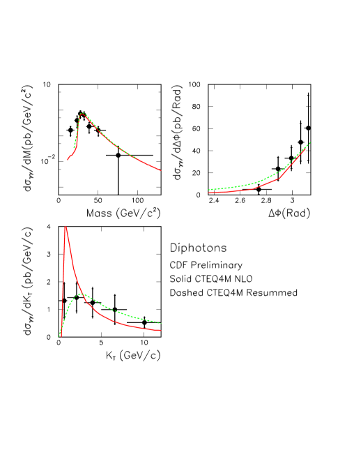
Figure 44: A comparison of the NLO and ResBos predictions for di-photon production at the Tevatron for the di-photon mass, the di-photon azimuthal angle (denoted here by $\Delta\phi$) and the di-photon transverse momentum (denoted here by $K_{T}$).

Phenomenology
Our understanding of photon pair production is already tested at the Tevatron [553, 554, 555]. A comparison of the CDF di-photon cross section to NLO and resummed predictions is shown in Fig. 44 (for a recent comparison with D$\not{\!0}$ data see, e.g., [237]). Measured inclusive observables, such as the invariant mass distribution, each photon’s $p_{T}$ distribution, the azimuthal angle ($\phi_{\gamma\gamma}$) distribution of pairs, agree reasonably well with NLO calculations [544, 545, 235, 546, 547, 237]. However, the measured di-photon $q_{T}$ distribution is noticeably broader than the NLO prediction, but it is in agreement with the resummed prediction of [236, 548]. This is expected since the $q_{T}$ distribution is particularly sensitive to soft gluon effects [196].

Figure 45: Top: di-photon differential cross section $d\sigma/dm_{\gamma\gamma}$ vs. $m_{\gamma\gamma}$ at LHC, with isolation criterion $E_{T\,max}=5$ GeV in $R=0.4$, for the scale choice $M=\mu=m_{\gamma\gamma}/2$. Bottom: factorization ($M$) and renormalization ($\mu$) scale dependences of the NLO cross section $d\sigma/dm_{\gamma\gamma}$ vs. $m_{\gamma\gamma}$, normalized by $d\sigma/dm_{\gamma\gamma}|_{M=\mu=m_{\gamma\gamma}/2}$.

The results from Run 1 at the Tevatron were obtained with less than 100 $pb^{-1}$ of data. During Run 2, a data sample approximately 20 times as large will be available, allowing both the di-photon signal and its background to be studied in detail. In particular, the di-photon $q_{T}$ distribution will be measured to much greater precision, allowing a study of the $q_{T}$ resummation techniques for a $gg$ initial state, necessary for both Higgs and di-photon production at the LHC [196].

On the theoretical side, scale ambiguities as well as the uncertainties from unknown beyond NLO corrections plague the predictions. A study of scale uncertainties has been performed [237] for inclusive observables such as the invariant mass distribution of photon pairs at LHC in the range 90 - 140 GeV, (Fig. 45). In the isolated case with $E_{T\,max}=5$ GeV inside a cone with $R=0.4$, the scale uncertainties are dominated by the dependences on the factorization and renormalization scales $M$ and $\mu$; while the fragmentation scale ($M_{f}$) dependence is negligible due to the strong suppression of the fragmentation contribution. The scale uncertainties are rather small (less than 5%) when the factorization and renormalization scales are set to be equal and are varied between $m_{\gamma\gamma}/2$ and $2m_{\gamma\gamma}$. On the other hand, anti-correlated variations of $M$ and $\mu$ in the same range lead to still rather large (up to 20%) uncertainties. In summary, the higher order corrections in prompt photon pair production are not fully under control yet. The consistent calculation at full NNLO accuracy would involve, in particular, two-loop $q\overline{q}\rightarrow\gamma\gamma$ amplitudes and the NNLO evolution of the parton distributions. Despite recent progress [288, 290, 289, 70] in this direction, such a NNLO description is not yet available. Furthermore, the box contribution $gg\rightarrow\gamma\gamma$ is the lowest order term of a new subprocess. Reducing its scale dependence would involve the calculation of N³LO corrections. Meanwhile, preliminary numerical comparisons have been initiated between these new NLO (and resummed) partonic calculations, and Monte Carlo event generators [196]. They have to be pushed further.

9.2.2 Reducible background

Before any cut is applied, most of the $H\rightarrow\gamma\gamma$ background comes from large-$p_{T}$ $\pi^{0}$, $\eta$ or $\omega$, decaying into photons. It can be severely reduced by imposing combined geometric and calorimetric isolation criteria. A small fraction of this huge background, consisting in large-$p_{T}$ isolated $\pi^{0}$ or $\eta$ may still pass such cuts. Earlier estimations of this background rely on Monte Carlo event generators, in which the tails of fragmentation distributions near the end point are rather poorly known. An improvement can be provided by using isolated $\pi^{0}$ pairs and $\gamma\pi^{0}$ Tevatron data, compared with Monte-Carlo type NLO calculations, such as [556], to improve NLO fragmentation functions at large $z$.

Like continuum di-photon production, its background from $\gamma\pi^{0}$ and $\pi^{0}\pi^{0}$ production has been extensively studied at the Tevatron [553, 554, 555]. This study can serve as a useful benchmark for the reducible background prediction, as well as for very useful tests of QCD. The inclusive $\pi^{0}\pi^{0}$ and $\gamma\pi^{0}$ cross sections are orders of magnitude larger than the $\gamma\gamma$ cross sections, making an extraction of the latter difficult, unless additional selection criteria are applied. As in essentially all collider photon measurements, an isolation cut needs to be applied to each of the di-photon candidates. In the case of CDF (in Run 1B), the isolation cut requires that any additional energy in a cone of radius R = 0.4 ($R=\sqrt{\Delta\eta^{2}+\Delta\phi^{2}}$) around the photon direction be less than 1 GeV. This requirement is basically saturated by the energy deposited by the di-photon underlying event and any additional minimum bias interactions that may have occurred during the same crossing. Such a strict isolation requirement rejects the majority of the $\gamma\pi^{0}$ and $\pi^{0}\pi^{0}$ backgrounds while retaining the true di-photon events with 80% efficiency.

The isolation cut suppresses the di-photon backgrounds to the point where they are comparable to the di-photon signal. One still needs a technique that allows for the separation of the di-photon signal from the background, in a Monte Carlo independent manner. CDF uses two such techniques: a measurement of the electro-magnetic shower width using a wire chamber placed at the EM shower maximum position, and a measurement of the fraction of the photon candidates that have converted in the magnet coil. The two photons from the $\pi^{0}$ can not be separately reconstructed given the tower granularity, but they do have a different shower width distribution and a different conversion probability than single photons. These differences allow the extraction of the di-photon signal, not on an event-by-event basis, but on a statistical basis, at each kinematic point being considered. The latter consideration is important since the background fraction does vary with the kinematics of the events being considered.

With the 1 GeV isolation cut for each photon, the di-photon signal fraction varies from about 30% at low $E_{T}$ to essentially 100% at high $E_{T}$ (50 GeV). The dominant source of background was determined to be from $\pi^{0}\pi^{0}$ production. Note that if the leakage of the electro-magnetic shower energy into the isolation cone is correctly accounted for, there is no reason to have a fractional isolation scale (some fixed fraction of the photon energy) rather than a fixed amount of energy allowed in the isolation cone. A fixed energy isolation cut provides a discrimination against jet backgrounds that increases in effectiveness as the energy of the photon candidate increases. At higher transverse energies, the isolation cut requires the jet to fragment into a $\pi^{0}$ at larger values of the fragmentation variable $z$, a process greatly suppressed by the steeply falling fragmentation function. The large $z$ ( $z>0.95$) region is poorly known since inclusive measurements of jet fragmentation [311] have few statistics in this region. This statement is even more true for the case of gluon jets, which form the bulk of the background source at the LHC. The di-photon trigger at the Tevatron selects those rare jets that fragment into isolated $\pi^{0}$’s. Thus, it would be useful to try to normalize the predictions of the event generators such as PYTHIA [115], which are used for background studies at the LHC to the background data at the Tevatron. Such a comparison is now in progress [557].

9.2.3 Production in association with jets

In order to improve the signal/background ratio, it has been suggested [549, 550] to study the associated production of $H(\rightarrow\gamma\gamma)+$ jet. For this process, both signal $S$ and background $B$ are reduced but still remain at the level of $\sim 100$ signal events at low LHC luminosity. The LO estimate has shown that the $S/B$ ratio is improved critically with the same level of significance $S/\sqrt{B}$. Furthermore, higher order corrections to the background have been shown recently [558] to be under better control than in the inclusive case.

Background: associated vs. inclusive
Indeed, the situations in the inclusive and associated channels are quite different. In the inclusive case, the main reason why the magnitude of the NNLO box contribution is comparable to the LO cross section is that the latter is initiated by $q\overline{q}$, whereas the former involves $gg$. The $gg$ luminosity, much larger than the $q\overline{q}$ one, compensates numerically the extra $\alpha_{s}^{2}$ factor of the box. This is not the case in the channel $\gamma\gamma$ + jet, since the LO cross section is dominated instead by a $qg$ initiated subprocess. The $qg$ luminosity is sizably larger than the $q\overline{q}$ one, which guarantees that the corresponding NNLO contribution remains small (less than 20% for $p_{T}>30$ GeV) compared to the LO result [558]. Thus, expecting that the subprocess $gg\rightarrow\gamma\gamma g$ gives the main NNLO correction, a quantitative description of the background with an accuracy better than 20% could be achieved already at NLO in the $\gamma\gamma$+ jet channel for a high-$p_{T}$ jet. All the helicity amplitudes needed for the implementation of the (“direct” contribution to the) background to NLO accuracy are now available [269, 559, 560].

Signal vs. background
The 3-body kinematics of the process allows more refined cuts to improve the $S/B$ ratio up to $1/2-1/3$ [549, 550] (to be compared with $S/B\geq 1/7$ for the inclusive channel). Due to helicity and total angular momentum conservation the $s$-wave state does not contribute to the dominant signal subprocess $gg\rightarrow Hg$. On the contrary, all angular momentum states contribute to the subprocesses $gq\rightarrow\gamma\gamma q$ and $q\overline{q}\rightarrow\gamma\gamma g$. Therefore, the signal has a more suppressed threshold behaviour compared to the background. The $S/B$ ratio can thus be improved by increasing the partonic c.m.s. energy $\sqrt{\hat{s}}$ far beyond threshold. Indeed, a cut $\sqrt{\hat{s}}>300$ GeV has been found to give the best S/B ratio for the LHC. The effect can not be fully explained by the threshold behavior only, since that would result in a uniform suppression factor. It was shown in [549, 550] (see Figs. 5 and 6 there) that the dependences of the background and the signal on the c.m.s. angular variables are quite different, therefore, the strong $\hat{s}$ cut affects them with different suppression factors (see [549, 550] for more details). This effect can be exploited to enhance the significance $S/\sqrt{B}$ at the same level as $S/B$. If the cut $\cos({\vartheta^{*})({j\gamma})}<-0.87$ on the jet-photon angle in the partonic c.m.s. is applied for $\sqrt{\hat{s}}<300$ GeV and combined with the cut $\sqrt{\hat{s}}>300$ GeV, the change on $S/B$ is rather small, while the significance is improved by a factor $\sim$ 1.3. The same effect can be observed with the cut on the jet angle $\vartheta^{*}({j})$ in the partonic c.m.s. (cf. the Fig. 5 mentioned above), but one should notice that the two variables, $\vartheta^{*}({j\gamma})$ and $\vartheta^{*}({j})$, are correlated. Therefore, it is desirable to perform a multi-variable optimization of the event selection. Notice that the present discussion is based on a LO analysis, and concerns only what was defined above as the “direct” component of the irreducible background. One now has to understand how this works at NLO.

Other, reducible, sources of background are potentially dangerous. The above-defined “single-fragmentation” component to the so-called irreducible background, and the reducible background coming from misidentification of jet events were treated on a similar footing in the LO analysis of [549, 550] as a de facto reducible background (see footnote 88). In [549, 550], a rough analysis found that this reducible background is less than 20% of the irreducible one after cuts are imposed. The misidentification rate is given mainly by the subprocesses $gq\rightarrow\gamma gq$, $gg\rightarrow\gamma q\overline{q}$ and $qq^{\prime}\rightarrow\gamma q(g)q^{\prime}(g)$, when the final state parton produces an energetic isolated photon but other products of the hadronization escape the detection as a jet. There, a $\gamma(\pi^{0})/\mbox{jet}$ rejection factor equal to 2500 for a jet misidentified as a photon and 5000 for a well separated $\gamma(\pi^{0})$ production by a jet were used. No additional $\pi^{0}$ rejection algorithms were applied. Furthermore, this reducible background is expected to be suppressed even more strongly than the irreducible background of “direct” type when a cut on $\sqrt{\hat{s}}$ is applied.

In summary, the associated channel $H(\rightarrow\gamma\gamma)+$ jet with jet transverse energy $E_{T}>30$ GeV and rapidity $|\eta|<4.5$ (thus involving forward hadronic calorimeters) opens a promising possibility for discovering the Higgs boson with a mass of 100-140 GeV at LHC even at low luminosity. However, to perform a quantitative analysis, the NLO calculations of the background have to be completed and included in a more realistic final state analysis.

Signal at NLO
The exact calculation of the NLO corrections to the signal is very complex, since the gluons interact with the Higgs boson via virtual quark loops. Fortunately, the effective field theory approach [561, 562] applicable in the large top mass limit with effective gluon-gluon-Higgs boson coupling gives an accurate approximation with an error less than 5%, provided $m_{H}\leq 2m_{t}$. Recently, in this approximation and using the helicity method, the transition amplitudes relevant to the NLO corrections have been analytically calculated for all contributing subprocesses (loop corrections [563] and bremsstrahlung [564, 565]). The subtraction method of [161, 227] has been used to cancel analytically the soft and collinear singularities and to implement the amplitudes into a numerical program of Monte-Carlo type which allows to calculate any infrared-safe observable for the production of a Higgs boson with one jet at NLO accuracy [197].

One of the main results of the calculation is that the NLO corrections are large and increase considerably the cross section, with a $K$ factor $\sim$ 1.5-1.6 ($K=\sigma^{NLO}/\sigma^{LO}$) and almost constant for a large kinematical range of $p_{T}$ and rapidity of the Higgs boson. Furthermore, the NLO result is less dependent on variations of the factorization and renormalization scales. Fig. 46(a) displays the $p_{T}$ distribution at both LO and NLO for a Higgs boson with $m_{H}=120$ GeV. The curves correspond to three different renormalization/factorization scale choices $Q=\mu\,(m_{H}^{2}+p_{T}^{2})^{1/2}$, with $\mu=0.5,1,2$, and show that the scale dependence is reduced at NLO. The same features can be observed in more detail in Fig. 46(b), where the LO and NLO cross sections integrated for $p_{T}$ larger than 30 and 70 GeV are shown as a function of the renormalization/factorization scale. Both the LO and NLO cross sections increase monotonically with decreasing $\mu$, down to the limiting value where perturbative QCD can still be applied, indicating that the stability of the NLO result is not completely satisfactory. However, in the usual range of variation of $\mu$ from 0.5 to 2, the LO scale uncertainty amounts to $\pm$ 35%, whereas at NLO it is reduced to $\pm$ 20%.

Figure 46: Scale dependence of LO and NLO distributions for Higgs boson production. (a) $p_{T}$ distributions at different scales and (b) the scale dependence of the integrated cross sections for $p_{T}>30$ and $70$ GeV. The MRST parton distributions are used.

9.3 Multi-lepton channels in the mass range $m_{H}\geq 140$ GeV.

Above 140 GeV, the most promising channel is $H\rightarrow ZZ^{(*)}\rightarrow 4$ leptons. The corresponding irreducible background comes mainly from the non resonant $ZZ^{(*)}$ production. Severe isolation cuts are needed to suppress reducible $t\overline{t}$ and $Zb\overline{b}$ backgrounds for Higgs boson masses below the $ZZ$ threshold. The topic of weak boson pair production is presented in a dedicated Section of the Electroweak Physics Chapter of this Report. In particular, the latter gathers the effects of NLO contributions to distributions of invariant mass, or transverse momentum of weak boson pairs, and comparisons between Monte Carlo event generators and recent NLO partonic calculations.

The $H\rightarrow WW\rightarrow 2l+\not{\!\!E}_{T}$ channels was recently found [566, 567] to be very promising in this mass range around 170 GeV, where the significance of the $H\rightarrow ZZ^{*}\rightarrow 4l$ channel is relatively small due to the suppression of $ZZ^{*}$ branching ratio as the $WW$ mode opens up. In this mass range, the leptonic branching ration of the $WW$ mode is approximately 100 times larger than the $ZZ^{*}\rightarrow 4l$ mode. Although the Higgs boson mass peak cannot be directly reconstructed in this case, the transverse mass distribution can be used to sign the Higgs boson and extract information on its mass.

The multileptonic channels $H\rightarrow WW^{(*)}$ and $H\rightarrow ZZ^{(*)}$ are also of great interest for the associated $WH$ production. Although the cross section for the associated production is a factor 50 to 100 lower than for the inclusive production, the $S/B$ ratio is substantially improved. They are also interesting to determine the Higgs boson couplings, since only the couplings to gauge bosons appear in the production and decay chain. The observability of $WH$ with $H\rightarrow WW^{*}\rightarrow 2l\;2\nu$ has been recently proposed in [568] and experimentally studied in [1]. The observability of the associated production $WH$, $H\rightarrow ZZ^{*}\rightarrow 4l$ has been recently considered in [569] and is sketched below. Due to the small number of events expected for $ZH$ and $t\overline{t}H$ production, only the $WH$ process has been investigated.

9.3.1 Associated $WH$ production, five lepton channel

Selection criteria
All simulations of Higgs boson and background events have been made with the PYTHIA 5.702 and JETSET 7.408 Monte Carlo programs implemented in the CMSIM/CMANA package [570]. The processes implemented in PYTHIA were simulated with parton showers, with the exception of internal bremsstrahlung, generated by PHOTOS [571]. No $K$ factors were used, so the final numbers of signal events may be underestimated by about a factor 1.3 [572]. The experimental resolution of CMS for lepton reconstruction was simulated by a Gaussian smearing:

$\Delta p_{T}/p_{T}=4.5\%\sqrt{p_{T}/1000}$  for muons,

$(\Delta E/E)^{2}=(4\%/\sqrt{E})^{2}+(0.230/E)^{2}+(0.55\%)^{2}$  for electrons,

where $p_{T}$ and $E$ are expressed in GeV. Dedicated programs calculate the dependence on $\eta$ and $p_{T}$ of the geometrical and kinematical acceptances, the invariant mass cuts to select the $Z$ or $Z^{*}$, and the rejection of non isolated leptons in jets with cuts selecting leptons without charged tracks above $p_{T}>$ 2 GeV in a cone $R<0.1$ ($R^{2}=\Delta\eta^{2}+\Delta\phi^{2}$). A few events were also fully generated and visualized in CMS by CMSIM. The reactions $W^{\pm}H\rightarrow\mu^{\pm}\nu_{\mu}ZZ^{(*)}\rightarrow 5\mu^{\pm}\nu_{\mu}$ and $W^{\pm}H\rightarrow e^{\pm}\nu_{e}ZZ^{(*)}\rightarrow 5e^{\pm}\nu_{e}$ have been studied in details. Although the branching ratios are identical, some differences between these channels are expected due to differences in acceptances and trigger efficiencies. The generated leptons are sorted in decreasing $p_{T}$ order, from 1 to 5, then the following cuts are applied.
For muon events :

• $\mid\eta\mid<2.1$ for $\mu_{1}$ and $\mu_{2}$ $\;\;\;\;\;\mid\eta\mid<2.5$ for $\mu_{3}$ to $\mu_{5}$

• $p_{T}>20$ GeV for $\mu_{1}$ $\;\;\;\;\;\;p_{T}>10$ GeV for $\mu_{2}$ $\;\;\;\;\;\;p_{T}>5$ or $10$ GeV for $\mu_{3},\mu_{4}$ and $\mu_{5}$

For electron events :

• $\mid\eta\mid<2.5$ for $e_{1}$ to $e_{5}$

• $p_{T}>20$ GeV for $e_{1}$ $\;\;\;\;\;\;p_{T}>15$ GeV for $e_{2}$ $\;\;\;\;\;\;p_{T}>7,10$ or $15$ GeV for $e_{3},e_{4}$ and $e_{5}$

Leptons 1 and 2 are the ones used to trigger events, leptons 3 to 5 $p_{T}$ thresholds can be set at lower values. Almost no difference is observed when the trigger threshold is set at a higher value (30 and 20 GeV), as expected since leptons 1 and 2 produced by $W$ and $Z$ decays are very energetic. The other possible final states: $2e+3\mu$, $2\mu+3e$, $4e+1\mu$ and $4\mu+1e$ are also good candidates. Since only small numerical differences were found in the results between the pure electronic and muonic final states, the 4 mixed ones were not simulated and the total number of expected events was multiplied by a factor 8. As the expected cross section is very low, the present search would be meaningful at high luminosity only. The pile-up at high luminosity has a minor impact for the detection of leptons. Nevertheless it has to be taken into account when using the isolation cuts.

	no cut	isolation cut	$Z$ mass cut	all cuts
$WH,M_{H}=150GeV$	3.56	3.42	2.89	2.69
$t\overline{t}$ background	141.	3.10	26.1	0.098
$Zb\overline{b}$ background	17.3	3.46	13.8	3.46
$WH,M_{H}=200GeV$	5.92	5.55	3.95	3.76
$WH,M_{H}=300GeV$	1.45	1.30	0.91	0.86
$t\overline{t}$ background	141.	3.10	0.098	0.098
$Zb\overline{b}$ background	17.3	3.46	1.73	0

Table 6: Number of events in the 5 leptons channel for $L=10^{5}pb^{-1}$, $p_{T}$ cut = 10 GeV. No mass window on 4 leptons is applied.

$H\rightarrow ZZ^{*}$
This channel concerns the mass range $m_{H}<2m_{Z}$. The irreducible background, due to the non resonant $WZZ^{*}$ production, is not included in PYTHIA. In order to get a rough order of magnitude, the $S/B$ ratio was then assumed to be of the same order as the one of direct production of $H\rightarrow ZZ^{*}$, compared to non resonant $ZZ^{*}$. This ratio has been estimated in [573] to be lower than 10 % for $m_{H}$ = 150 GeV. The reducible background comes from the $t\overline{t}$ and $Zb\overline{b}$ channels with three leptons coming from semi-leptonic decays of $B$ and $D$ mesons. The initial cross sections of these processes are very high and, without cut, this background is much higher than the irreducible one.

The selection requests one pair of opposite sign muons or electrons with a mass equal to $m_{Z}\pm 5$ GeV, and one pair of opposite sign muons or electrons with a mass below $m_{Z}$. This removes only 19 % of the signal events which fall in the tails of the mass distributions. An additional effect of widening the Z mass would come from the $e^{\pm}$ bremsstrahlung in the tracker material [574] and contribute to decrease the acceptance. The lepton pair mass spectra of the $t\overline{t}$ and $Zb\overline{b}$ backgrounds exhibit a peak at low mass. A cut at $m_{Z^{*}}>10$ GeV would further reduce these backgrounds by 20 % without affecting the signal. No detector reconstruction inefficiency was considered at this level. The isolation cut is used to reject leptons from $b$ or $c$ quark decay, in the reducible background channels. The events exhibiting tracks with $p_{T}>2$ GeV contained in a cone $R<$ 0.1 around any of the five leptons are rejected (Fig. 47). Actually a better rejection is expected in the CMS detector when using the information from the $b$ vertex position [575].

Another reducible background was considered: the non resonant production of $ZZ^{*}$ where one of the $Z^{(*)}$ decays into two leptons and the other decays into $b\overline{b}$, the $b$ quarks decaying semi-leptonically. The number of events before acceptance, mass and isolation cut is about 70 % of the signal, but as we expect the leptons from the $b$’s to be very soft and non isolated, that this background can be considered as negligible.

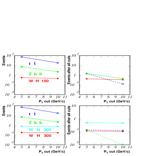
Figure 47: Number of events at $L=10^{5}pb^{-1}$ for $WH\rightarrow 5\mu$ channel and background for M_H = 150 GeV (top), 200 and 300 GeV (bottom) after kinematical cuts (left), isolation and $ZZ$ mass cuts combined (right). $P_{T}$ cut refers to the softest of the five muons. Dotted line is an upper limit (no Monte Carlo event survive the cuts).

$H\rightarrow ZZ$
This channel is similar to the previous one except that we request two pairs of opposite sign muons or electrons with masses equal to $m_{Z}\pm 5$ GeV. This cut removes 32 to 34 % of the signal events. It is now much more efficient against the $t\overline{t}$ background than against the $Zb\overline{b}$, because the $Zb\overline{b}$ channel involves a real $Z$. The calculations were made for Higgs bosons with $m_{H}=200$ and 300 GeV (Fig. 47). The acceptances of the signal vary only slightly as a function of $p_{T}$ cut and other selection cuts. The four leptons mass spectrum for the background is a wide distribution centered around 150 GeV. A cut on this spectrum can be used to obtain an additional rejection factor of the order of 10 to 50, after the Higgs boson mass has been previously measured in a more sensitive channel, like the inclusive $H\rightarrow 4l$ [575].

Results
The number of expected 5 muons or 5 electrons events for one year of running at high luminosity $100fb^{-1}$ is low: 0.34 for a Higgs boson mass of 150 GeV, 0.47 for 200 GeV and 0.11 for 300 GeV/c. Considering all the possible 5 leptons channels, these numbers must be multiplied by a factor 8. They are summarized in table 1, together with the corresponding backgrounds (not including the cut on the four leptons mass spectrum described above). The $S/B$ ratio is better for $m_{H}=200$ GeV and is unacceptable for $m_{H}=150$ GeV. Thus this channel can be considered almost hopeless for the discovery of the Higgs boson below the $ZZ$ threshold. On the other hand, if the Higgs boson is in the mass range 200 to 300 GeV, the detection of these rare 5 lepton events above a low background would be a valuable information for the study of the Higgs boson couplings.

However, before drawing any definitive conclusion, several issues should be improved concerning the backgrounds. Firstly the irreducible $WZZ^{*}$ background has to be calculated, e.g. using an automatized calculation like [138] and included in the analysis. Moreover the reducible $Zb\overline{b}$ process should be revisited with another Monte Carlo generator, as the implementation in PYTHIA 5.7 for the $Zb\overline{b}$ process is known to suffer from an instability in the phase space generation (this implementation has been removed from the version PYTHIA 6.1 for this reason). Finally, another source of 5 leptons events, not evaluated with enough statistics so far is the semi-leptonic decay of $b\overline{b}$ or $c\overline{c}$ generated by initial or final gluon radiation.

An extension of this study would also be the investigation of the associated production of a higher mass Higgs boson using other decay modes with larger branching ratios like $Z\rightarrow$ jet jet.

References

- [1] ATLAS Collaboration, ATLAS Detector and Physics Performance Technical Design Report, CERN/LHCC/99-14 and CERN/LHCC/99-15 (1999).
- [2] Proceedings of the “LHC workshop”, Aachen 1990, G. Jarlskog and D. Rein editors, report CERN 90-10.
- [3] TOTEM Collaboration, Technical Proposal, CERN/LHCC/99-7 (1999).
- [4] See R.K. Ellis, W.J. Stirling and B.R. Webber, QCD and collider physics (Cambridge University Press, Cambridge, 1996), and references therein.
- [5] See J.C. Collins, D.E. Soper and G. Sterman, in Perturbative Quantum Chromodynamics, ed. A.H. Mueller (World Scientific, Singapore, 1989), p. 1, and references therein.
- [6] S. D. Ellis, Z. Kunszt and D. E. Soper, Phys. Rev. Lett. 69 (1992) 1496.
- [7] H. L. Lai et al. [CTEQ Collaboration], Eur. Phys. J. C12 (2000) 375 [hep-ph/9903282].
- [8] S. Catani, Y. L. Dokshitzer, M. H. Seymour and B. R. Webber, Nucl. Phys. B406 (1993) 187.
- [9] S. D. Ellis and D. E. Soper, Phys. Rev. D48 (1993) 3160 [hep-ph/9305266].
- [10] A. D. Martin, R. G. Roberts, W. J. Stirling and R. S. Thorne, hep-ph/9907231.
- [11] O. V. Tarasov, A. A. Vladimirov and A. Y. Zharkov, Phys. Lett. B93 (1980) 429.
- [12] T. van Ritbergen, J. A. Vermaseren and S. A. Larin, Phys. Lett. B400 (1997) 379 [hep-ph/9701390].
- [13] C. Caso et al., Eur. Phys. J. C3 (1998) 1, and 1999 off-year partial update for the 2000 edition available on the PDG WWW pages (URL: http://pdg.lbl.gov/).
- [14] V. N. Gribov and L. N. Lipatov, Sov. J. Nucl. Phys. 15 (1972) 438.
- [15] V. N. Gribov and L. N. Lipatov, Sov. J. Nucl. Phys. 15 (1972) 675.
- [16] G. Altarelli and G. Parisi, Nucl. Phys. B126 (1977) 298.
- [17] Yu. L. Dokshitzer, Sov. Phys. JETP 46 (1977) 641.
- [18] E. G. Floratos, D. A. Ross and C. T. Sachrajda, Nucl. Phys. B129 (1977) 66, E ibid. B139 (1978) 545.
- [19] E. G. Floratos, D. A. Ross and C. T. Sachrajda, Nucl. Phys. B152 (1979) 493.
- [20] A. Gonzalez-Arroyo, C. Lopez and F. J. Yndurain, Nucl. Phys. B153 (1979) 161.
- [21] A. Gonzalez-Arroyo and C. Lopez, Nucl. Phys. B166 (1980) 429.
- [22] G. Curci, W. Furmanski and R. Petronzio, Nucl. Phys. B175 (1980) 27.
- [23] W. Furmanski and R. Petronzio, Phys. Lett. B97 (1980) 437.
- [24] E. G. Floratos, C. Kounnas and R. Lacaze, Nucl. Phys. B192 (1981) 417.
- [25] S. A. Larin, T. van Ritbergen and J. A. Vermaseren, Nucl. Phys. B427 (1994) 41.
- [26] S. A. Larin, P. Nogueira, T. van Ritbergen and J. A. Vermaseren, Nucl. Phys. B492 (1997) 338 [hep-ph/9605317].
- [27] G. Altarelli, R. K. Ellis and G. Martinelli, Nucl. Phys. B157 (1979) 461.
- [28] A. D. Martin, R. G. Roberts, W. J. Stirling and R. S. Thorne, Eur. Phys. J. C4 (1998) 463 [hep-ph/9803445].
- [29] S. Alekhin, hep-ph/9910490.
- [30] S. I. Alekhin, hep-ph/9912484.
- [31] T. Matsuura, R. Hamberg and W. L. van Neerven, Nucl. Phys. B345 (1990) 331.
- [32] R. Hamberg, W. L. van Neerven and T. Matsuura, Nucl. Phys. B359 (1991) 343.
- [33] W. L. van Neerven and E. B. Zijlstra, Nucl. Phys. B382 (1992) 11.
- [34] J. Blumlein, S. Riemersma, M. Botje, C. Pascaud, F. Zomer, W. L. van Neerven and A. Vogt, hep-ph/9609400.
- [35] W. T. Giele and S. Keller, Phys. Rev. D58 (1998) 094023 [hep-ph/9803393].
- [36] S. Alekhin, Eur. Phys. J. C10 (1999) 395 [hep-ph/9611213].
- [37] R.D. Ball and J. Huston, in the proceedings of the Les Houches Workshop ‘Physics at TeV Colliders’, June 1999.
- [38] G. D’Agostini, hep-ph/9512295.
- [39] G. D’Agostini, CERN-99-03.
- [40] Parton Distribution working group of the QCD and Weak Boson Physics workshop in preparation for Run II at the Fermilab Tevatron, March 1999-January 2000
- [41] Workshop on ‘Confidence Limits’, 17-18 January 2000, CERN, organized by F. James and L. Lyons.
- [42] D. A. Kosower, Nucl. Phys. B520 (1998) 263 [hep-ph/9708392].
- [43] D. A. Kosower, Nucl. Phys. B506 (1997) 439 [hep-ph/9706213].
- [44] Fig. 21 in Ref. [28]: S.K. thanks W.J. Stirling for pointing this out.
- [45] L. W. Whitlow, E. M. Riordan, S. Dasu, S. Rock and A. Bodek, Phys. Lett. B282 (1992) 475.
- [46] A. C. Benvenuti et al. [BCDMS Collaboration], Phys. Lett. B223 (1989) 485.
- [47] A. C. Benvenuti et al. [BCDMS Collaboration], Phys. Lett. B237 (1990) 592.
- [48] M. Arneodo et al. [New Muon Collaboration], Nucl. Phys. B483 (1997) 3 [hep-ph/9610231].
- [49] M. R. Adams et al. [E665 Collaboration], Phys. Rev. D54 (1996) 3006.
- [50] S. Aid et al. [H1 Collaboration], Nucl. Phys. B470 (1996) 3 [hep-ex/9603004].
- [51] M. Derrick et al. [ZEUS Collaboration], Z. Phys. C72 (1996) 399 [hep-ex/9607002].
- [52] J. Blumlein and W. L. van Neerven, Phys. Lett. B450 (1999) 412 [hep-ph/9811519].
- [53] G.B. West, Annal. Phys. 74 (1972) 464.
- [54] J. Gomes et al., Phys. Rev. D49 (1994) 4348.
- [55] W. Melnitchouk, I. R. Afnan, F. Bissey and A. W. Thomas, hep-ex/9912001.
- [56] U. K. Yang and A. Bodek, hep-ph/9912543.
- [57] T. Adams et al. [NuTeV Collaboration], hep-ex/9906037.
- [58] A. L. Kataev, G. Parente and A. V. Sidorov, hep-ph/9905310.
- [59] A. L. Kataev, G. Parente and A. V. Sidorov, hep-ph/9907310.
- [60] http:www.ihep.sualekhinpdf99.
- [61] W. L. van Neerven and E. B. Zijlstra, Phys. Lett. B272 (1991) 127.
- [62] E. B. Zijlstra and W. L. van Neerven, Phys. Lett. B273 (1991) 476.
- [63] E. B. Zijlstra and W. L. van Neerven, Phys. Lett. B297 (1992) 377.
- [64] E. B. Zijlstra and W. L. van Neerven, Nucl. Phys. B383 (1992) 525.
- [65] J. Blumlein and A. Vogt, Phys. Lett. B370 (1996) 149 [hep-ph/9510410].
- [66] S. Catani and F. Hautmann, Nucl. Phys. B427 (1994) 475 [hep-ph/9405388].
- [67] V. S. Fadin and L. N. Lipatov, Phys. Lett. B429 (1998) 127 [hep-ph/9802290].
- [68] J. Blumlein and A. Vogt, Phys. Rev. D58 (1998) 014020 [hep-ph/9712546].
- [69] J. Blumlein, V. Ravindran, W. L. van Neerven and A. Vogt, hep-ph/9806368.
- [70] W. L. van Neerven and A. Vogt, hep-ph/9907472.
- [71] W.L. van Neerven and A. Vogt, INLO-PUB 04/00 (to appear)
- [72] J. A. Gracey, Phys. Lett. B322 (1994) 141 [hep-ph/9401214].
- [73] J. F. Bennett and J. A. Gracey, Nucl. Phys. B517 (1998) 241 [hep-ph/9710364].
- [74] E. B. Zijlstra and W. L. van Neerven, Nucl. Phys. B417 (1994) 61.
- [75] For a recent review, see M. Beneke, Phys. Rept. 317 (1999) 1 [hep-ph/9807443].
- [76] Y. L. Dokshitzer, G. Marchesini and B. R. Webber, Nucl. Phys. B469 (1996) 93 [hep-ph/9512336].
- [77] D. V. Shirkov and I. L. Solovtsov, Phys. Rev. Lett. 79 (1997) 1209 [hep-ph/9704333].
- [78] I. L. Solovtsov and D. V. Shirkov, Theor. Math. Phys. 120 (1999) 1220 [hep-ph/9909305].
- [79] A. L. Kataev, A. V. Kotikov, G. Parente and A. V. Sidorov, Phys. Lett. B388 (1996) 179 [hep-ph/9605367].
- [80] A. L. Kataev, A. V. Kotikov, G. Parente and A. V. Sidorov, Phys. Lett. B417 (1998) 374 [hep-ph/9706534].
- [81] W. G. Seligman et al., Phys. Rev. Lett. 79 (1997) 1213.
- [82] M. Dasgupta and B. R. Webber, Phys. Lett. B382 (1996) 273 [hep-ph/9604388].
- [83] G. Parisi and N. Sourlas, Nucl. Phys. B151 (1979) 421.
- [84] I. S. Barker, C. S. Langensiepen and G. Shaw, Nucl. Phys. B186 (1981) 61.
- [85] J. Chyla and J. Rames, Z. Phys. C31 (1986) 151.
- [86] V. G. Krivokhizhin, S. P. Kurlovich, V. V. Sanadze, I. A. Savin, A. V. Sidorov and N. B. Skachkov, Z. Phys. C36 (1987) 51.
- [87] V. G. Krivokhizhin et al., Z. Phys. C48 (1990) 347.
- [88] S. A. Larin and J. A. Vermaseren, Phys. Lett. B303 (1993) 334 [hep-ph/9302208].
- [89] G. Parente, A. V. Kotikov and V. G. Krivokhizhin, Phys. Lett. B333 (1994) 190 [hep-ph/9405290].
- [90] J.A.M. Vermaseren, private communication to A.L.K., W.L. van Neerven and A. Vogt, November 1999.
- [91] M. Virchaux and A. Milsztajn, Phys. Lett. B274 (1992) 221.
- [92] V.A. Matveev, R.M. Muradyan, A.N. Tavkhelidze, Lett. Nuov. Cim. 7 (1973) 719.
- [93] S. J. Brodsky and G. R. Farrar, Phys. Rev. Lett. 31 (1973) 1153.
- [94] E. L. Berger and S. J. Brodsky, Phys. Rev. Lett. 42 (1979) 940.
- [95] J. F. Gunion, P. Nason and R. Blankenbecler, Phys. Rev. D29 (1984) 2491.
- [96] W. Bernreuther and W. Wetzel, Nucl. Phys. B197 (1982) 228; Err. ibid. B513 (1998) 758.
- [97] S. A. Larin, T. van Ritbergen and J. A. Vermaseren, Nucl. Phys. B438 (1995) 278 [hep-ph/9411260].
- [98] K. G. Chetyrkin, B. A. Kniehl and M. Steinhauser, Phys. Rev. Lett. 79 (1997) 2184 [hep-ph/9706430].
- [99] J. Santiago and F. J. Yndurain, Nucl. Phys. B563 (1999) 45 [hep-ph/9904344].
- [100] F. J. Yndurain, Phys. Lett. B74 (1978) 68.
- [101] M. Dittmar, F. Pauss and D. Zurcher, Phys. Rev. D56 (1997) 7284 [hep-ex/9705004].
- [102] F. Behner, Talk given at International Europhysics Conference on High-Energy Physics (HEP 97), Jerusalem, Israel, 19-26 Aug 1997.
- [103] P. Chiappetta, G. J. Gounaris, J. Layssac and F. M. Renard, Phys. Rev. D59 (1999) 014016 [hep-ph/9807563].
- [104] D. Bandourin, V. Konoplyannikov, N. Skachkov; Using photon–jet final states to constrain the gluon luminosity at the LHC, CMS note in preparation.
- [105] M. Dittmar and K. Mazumdar; the possibility to measure the charm, beauty and strange quark luminosity at the LHC; CMS note in preparation.
- [106] S.D. Drell and T. Yan, Phys. Rev. Lett. 25 (1970) 316.
- [107] E.L. Berger, L.E. Gordon and M. Klasen, Phys. Rev. D58 (1998) 074012, hep-ph/9803387;
- [108] E. L. Berger and M. Klasen, hep-ph/9906402.
- [109] M. Klasen, G. Kramer and B. Pötter, Eur. Phys. J. C1 (1998) 261, hep-ph/9703302.
- [110] P.B. Arnold and R.P. Kauffman, Nucl. Phys. B349 (1991) 381.
- [111] H.L. Lai et al., Phys. Rev. D55 (1997) 1280, hep-ph/9606399.
- [112] C. Albajar et al. [UA1 Collaboration], Phys. Lett. 209B (1988) 397.
- [113] M. Glück, E. Reya and A. Vogt, Eur. Phys. J. C5 (1998) 461, hep-ph/9806404.
- [114] M. Glück, E. Reya and A. Vogt, Z. Phys. C53 (1992) 127.
- [115] T. Sjostrand, Comput. Phys. Commun. 82 (1994) 74.
- [116] G. Marchesini, B. R. Webber, G. Abbiendi, I. G. Knowles, M. H. Seymour and L. Stanco, Comput. Phys. Commun. 67 (1992) 465.
- [117] G. Marchesini, B. R. Webber, G. Abbiendi, I. G. Knowles, M. H. Seymour and L. Stanco, hep-ph/9607393.
- [118] G. Corcella et al., hep-ph/9912396.
- [119] F. E. Paige, S. D. Protopopescu, H. Baer and X. Tata, hep-ph/9810440.
- [120] H. Baer, F. E. Paige, S. D. Protopopescu and X. Tata, hep-ph/0001086.
- [121] Z. Kunszt and W. J. Stirling, Phys. Rev. D37 (1988) 2439.
- [122] F. A. Berends and H. Kuijf, Nucl. Phys. B353 (1991) 59.
- [123] F. A. Berends, H. Kuijf, B. Tausk and W. T. Giele, Nucl. Phys. B357 (1991) 32.
- [124] F. A. Berends and W. T. Giele, Nucl. Phys. B306 (1988) 759.
- [125] M. L. Mangano and S. J. Parke, Phys. Rept. 200 (1991) 301.
- [126] P. De Causmaecker, R. Gastmans, W. Troost and T. T. Wu, Nucl. Phys. B206 (1982) 53.
- [127] F. A. Berends, R. Kleiss, P. De Causmaecker, R. Gastmans, W. Troost and T. T. Wu, Nucl. Phys. B206 (1982) 61.
- [128] F. A. Berends, P. De Causmaecker, R. Gastmans, R. Kleiss, W. Troost and T. T. Wu [CALKUL Collaboration], Nucl. Phys. B264 (1986) 265.
- [129] S. Dittmaier, Phys. Rev. D59 (1999) 016007 [hep-ph/9805445].
- [130] H. Tanaka, T. Kaneko and Y. Shimizu, Comput. Phys. Commun. 64 (1991) 149.
- [131] T. Ishikawa et al., GRACE manual, KEK Report 92-19, February 1993; see also [132].
-
[132]
An extensive reference list for CompHEP and Grace
can be found at:
http://wwwlapp.in2p3.fr/cpp/papers/preprints/preprints.html - [133] T. Stelzer and W. F. Long, Comput. Phys. Commun. 81 (1994) 357 [hep-ph/9401258].
- [134] F. Caravaglios and M. Moretti, Phys. Lett. B358 (1995) 332 [hep-ph/9507237].
- [135] A. Ballestrero and E. Maina, Phys. Lett. B350 (1995) 225 [hep-ph/9403244].
- [136] E. Accomando and A. Ballestrero, Comput. Phys. Commun. 99 (1997) 270 [hep-ph/9607317].
- [137] F. Caravaglios, M. L. Mangano, M. Moretti and R. Pittau, Nucl. Phys. B539 (1999) 215 [hep-ph/9807570].
- [138] A. Pukhov et al., hep-ph/9908288.
- [139] F. Yuasa, D. Perret-Gallix, S. Kawabata and T. Ishikawa, Nucl. Instrum. Meth. A389 (1997) 77.
- [140] F. Yuasa, Y. Kurihara and S. Kawabata, Phys. Lett. B414 (1997) 178 [hep-ph/9706225].
- [141] G. P. Lepage, J. Comput. Phys. 27 (1978) 192.
- [142] W.H. Press, S.A. Teukolsky, W.T. Vetterling and B.P. Flannery, Numerical Recipes in Fortran (Cambridge University Press, Cambridge, 1992).
- [143] S. Kawabata, Comput. Phys. Commun. 41 (1986) 127.
- [144] S. Kawabata, Comput. Phys. Commun. 88 (1995) 309.
- [145] G.I. Manankova, A.F. Tatarchenko and F.V. Tkachov, Contribution to AIHENP-95, Pisa, Italy, April 3-8, 1995 (extended version).
- [146] S. Jadach, physics/9910004.
- [147] V. A. Ilyin, D. N. Kovalenko and A. E. Pukhov, Int. J. Mod. Phys. C7 (1996) 761 [hep-ph/9612479].
- [148] F. A. Berends, R. Pittau and R. Kleiss, Comput. Phys. Commun. 85 (1995) 437 [hep-ph/9409326].
- [149] D. N. Kovalenko and A. E. Pukhov, Nucl. Instrum. Meth. A389 (1997) 299.
- [150] G. Corcella and M. H. Seymour, Phys. Lett. B442 (1998) 417 [hep-ph/9809451].
- [151] J. Andre and T. Sjostrand, Phys. Rev. D57 (1998) 5767 [hep-ph/9708390].
- [152] G. Mahlon and S. Parke, hep-ph/9912458.
- [153] R. K. Ellis, G. Marchesini and B. R. Webber, Nucl. Phys. B286 (1987) 643, Erratum Nucl. Phys. B294 (1987) 1180.
- [154] J. Fujimoto et al., Comput. Phys. Commun. 100 (1997) 128 [hep-ph/9605312].
- [155] K. Odagiri, JHEP 9810 (1998) 006 [hep-ph/9806531].
- [156] H. Dreiner, P. Richardson and M. H. Seymour, hep-ph/9912407.
- [157] J. Kublbeck, M. Bohm and A. Denner, Comput. Phys. Commun. 60 (1990) 165.
- [158] R. Mertig, M. Bohm and A. Denner, Comput. Phys. Commun. 64 (1991) 345.
- [159] T. Hahn, hep-ph/9905354.
- [160] W. T. Giele and E. W. Glover, Phys. Rev. D46 (1992) 1980.
- [161] S. Frixione, Z. Kunszt and A. Signer, Nucl. Phys. B467 (1996) 399 [hep-ph/9512328].
- [162] S. Catani and M. H. Seymour, Nucl. Phys. B485 (1997) 291 [hep-ph/9605323], Erratum Nucl. Phys. 510 (1997) 503.
- [163] M. H. Seymour, Comput. Phys. Commun. 90 (1995) 95 [hep-ph/9410414].
- [164] G. Corcella and M. H. Seymour, Nucl. Phys. B565 (2000) 227 [hep-ph/9908388].
- [165] G. Miu and T. Sjostrand, Phys. Lett. B449 (1999) 313 [hep-ph/9812455].
- [166] S. Mrenna, hep-ph/9902471.
- [167] C. Friberg and T. Sjostrand, hep-ph/9906316.
- [168] J. Collins, hep-ph/0001040.
- [169] T. Sjostrand, Phys. Lett. B157 (1985) 321.
- [170] M. Bengtsson, T. Sjostrand and M. van Zijl, Z. Phys. C32 (1986) 67.
- [171] G. Marchesini and B. R. Webber, Nucl. Phys. B310 (1988) 461.
- [172] S. Catani, B. R. Webber and G. Marchesini, Nucl. Phys. B349 (1991) 635.
- [173] A. Del Fabbro and D. Treleani, hep-ph/9911358.
- [174] A. Kulesza and W. J. Stirling, hep-ph/9912232.
- [175] F. Abe et al. [CDF Collaboration], Phys. Rev. Lett. 79 (1997) 584.
- [176] F. Abe et al. [CDF Collaboration], Phys. Rev. D56 (1997) 3811.
- [177] G. Calucci and D. Treleani, Phys. Rev. D57 (1998) 602 [hep-ph/9708233].
- [178] G. Calucci and D. Treleani, Phys. Rev. D60 (1999) 054023 [hep-ph/9902479].
- [179] G. Calucci and D. Treleani, Nucl. Phys. Proc. Suppl. 71 (1999) 392 [hep-ph/9711225].
- [180] L. Lonnblad, Comput. Phys. Commun. 118 (1999) 213 [hep-ph/9810208].
- [181] Lynn Garren, StdHepC++, http://www-pat.fnal.gov/stdhep/c++/
- [182] F. Krauss, R. Kuhn and G. Soff, Acta Phys. Polon. B30 (1999) 3875 [hep-ph/9909572].
- [183] A. Donnachie and P. V. Landshoff, Phys. Lett. B296 (1992) 227 [hep-ph/9209205].
- [184] G. J. Alner et al. [UA5 Collaboration], Nucl. Phys. B291 (1987) 445.
- [185] V. A. Abramovsky, V. N. Gribov and O. V. Kancheli, Sov. J. Nucl. Phys. 18 (1974) 308.
- [186] G. Marchesini and B. R. Webber, Phys. Rev. D38 (1988) 3419.
- [187] B. Abbott et al. [D0 Collaboration], Phys. Rev. Lett. 80 (1998) 5498 [hep-ex/9803003].
- [188] T. Affolder et al. [CDF Collaboration], Phys. Rev. Lett. 84 (2000) 845 [hep-ex/0001021].
- [189] G. Corcella and M.H. Seymour, hep-ph/9911536.
- [190] S. Frixione, P. Nason and G. Ridolfi, collisions,” Nucl. Phys. B542 (1999) 311 [hep-ph/9809367].
- [191] R. K. Ellis and S. Veseli, Nucl. Phys. B511 (1998) 649 [hep-ph/9706526].
- [192] J. C. Collins, D. E. Soper and G. Sterman, Nucl. Phys. B250 (1985) 199.
- [193] C. Balazs, J. Huston and I. Puljak, hep-ph/0002032.
- [194] C. Balazs and C. P. Yuan, Phys. Rev. D56 (1997) 5558 [hep-ph/9704258].
- [195] C. Balazs and C. P. Yuan, hep-ph/0001103.
- [196] Proceedings of Les Houches Workshop on Physics at TeV Colliders, 1999, QCD Working Group (Conveners S. Catani, M. Dittmar, J. Huston, D. Soper and S. Tapprogge), eds. P. Aurenche, G. Belanger, F. Boudjema, J.P. Guillet and E. Pilon, to be available on hep-ph.
- [197] D. de Florian, M. Grazzini and Z. Kunszt, Phys. Rev. Lett. 82 (1999) 5209 [hep-ph/9902483].
- [198] Pythia manual update for version 6.1.
- [199] D. Denegri, private communication.
- [200] A. D. Martin, W. J. Stirling and R. G. Roberts, Phys. Lett. B354 (1995) 155 [hep-ph/9502336].
- [201] A.E. Pukhov et al., CompHEP v.41, to appear.
- [202] T. Abe, J. Fujimoto, T. Ishikawa, Y. Kurihara, K. Kato and T. Watanabe, Prepared for Workshop on Monte Carlo Generators for HERA Physics, Hamburg, Germany, 27-30 Apr 1998.
- [203] J. Kalinowski, K. Konishi, P. N. Scharbach and T. R. Taylor, Nucl. Phys. B181 (1981) 253.
- [204] J. Kalinowski, K. Konishi and T. R. Taylor, Nucl. Phys. B181 (1981) 221.
- [205] K. Kato and T. Munehisa, Phys. Rev. D36 (1987) 61.
- [206] M. Mangano, S. Parke and Z. Xu, FERMILAB-CONF-87/78-T Presented at Les Rencontres de Physique de la Vallee d’Aoste, La Thuile, Italy, Mar 1-7, 1987 .
- [207] F. A. Berends and W. Giele, Nucl. Phys. B294 (1987) 700.
- [208] M. Mangano, S. Parke and Z. Xu, Nucl. Phys. B298 (1988) 653.
- [209] S. J. Parke and T. R. Taylor, Phys. Rev. Lett. 56 (1986) 2459.
- [210] J. C. Collins, Nucl. Phys. B304 (1988) 794.
- [211] I. G. Knowles, Nucl. Phys. B310 (1988) 571.
- [212] P.N. Burrows et al., hep-ex/9612012, Presented at 1996 DPF / DPB Summer Study on New Directions for High-Energy Physics (Snowmass 96).
- [213] M. Schmelling, hep-ex/9701002, Talk given at 28th International Conference on High-energy Physics (ICHEP 96), Warsaw, Poland.
- [214] S. Catani, hep-ph/9712442, in Proc. of the XVIII International Symposium on Lepton-Photon Interactions, LP97, eds. A. De Roeck and A. Wagner (World Scientific, Singapore, 1998), p. 147, and references therein.
- [215] S. Bethke, hep-ex/0001023, Lectures given at International Summer School on Particle Production Spanning MeV and TeV Energies (Nijmegen 99), Nijmegen, Netherlands.
- [216] L. N. Lipatov, Sov. J. Nucl. Phys. 20 (1975) 94.
- [217] D. R. Yennie, S. C. Frautschi and H. Suura, Annals Phys. 13 (1961) 379.
- [218] A. Bassetto, M. Ciafaloni and G. Marchesini, Phys. Rept. 100 (1983) 201.
- [219] F. A. Berends and W. T. Giele, Nucl. Phys. B313 (1989) 595.
- [220] Z. Kunszt and D. E. Soper, Phys. Rev. D46 (1992) 192.
- [221] Z. Kunszt, A. Signer and Z. Trocsanyi, Nucl. Phys. B420 (1994) 550 [hep-ph/9401294].
- [222] W. T. Giele, E. W. Glover and D. A. Kosower, Nucl. Phys. B403 (1993) 633 [hep-ph/9302225].
- [223] E. W. Glover and M. R. Sutton, Phys. Lett. B342 (1995) 375 [hep-ph/9410234].
- [224] S. Keller and E. Laenen, Phys. Rev. D59 (1999) 114004 [hep-ph/9812415].
- [225] Z. Nagy and Z. Trocsanyi, Nucl. Phys. B486 (1997) 189 [hep-ph/9610498].
- [226] S. Catani and M. H. Seymour, Phys. Lett. B378 (1996) 287 [hep-ph/9602277].
- [227] S. Frixione, Nucl. Phys. B507 (1997) 295 [hep-ph/9706545].
- [228] W. B. Kilgore and W. T. Giele, hep-ph/9903361.
- [229] H. Baer, J. Ohnemus and J. F. Owens, Phys. Rev. D42 (1990) 61.
- [230] L. E. Gordon and W. Vogelsang, Phys. Rev. D50 (1994) 1901.
- [231] S. Frixione, hep-ph/9809397.
- [232] S. Frixione, Phys. Lett. B429 (1998) 369 [hep-ph/9801442].
- [233] F. Aversa, P. Chiappetta, M. Greco and J. P. Guillet, Nucl. Phys. B327 (1989) 105.
- [234] P. Aurenche, R. Baier, M. Fontannaz and D. Schiff, Nucl. Phys. B297 (1988) 661.
- [235] B. Bailey, J. F. Owens and J. Ohnemus, Phys. Rev. D46 (1992) 2018.
- [236] C. Balazs, E. L. Berger, S. Mrenna and C. P. Yuan, Phys. Rev. D57 (1998) 6934 [hep-ph/9712471].
- [237] T. Binoth, J. P. Guillet, E. Pilon and M. Werlen, hep-ph/9911340. See also [196].
- [238] U. Baur, T. Han and J. Ohnemus, Phys. Rev. D48 (1993) 5140 [hep-ph/9305314].
- [239] U. Baur, T. Han and J. Ohnemus, Phys. Rev. D57 (1998) 2823 [hep-ph/9710416].
- [240] D. De Florian and A. Signer, hep-ph/0002138.
- [241] J. Ohnemus and J. F. Owens, Phys. Rev. D43 (1991) 3626.
- [242] J. Ohnemus, Phys. Rev. D44 (1991) 1403.
- [243] J. Ohnemus, Phys. Rev. D44 (1991) 3477.
- [244] U. Baur, T. Han and J. Ohnemus, Phys. Rev. D51 (1995) 3381 [hep-ph/9410266].
- [245] U. Baur, T. Han and J. Ohnemus, Phys. Rev. D53 (1996) 1098 [hep-ph/9507336].
- [246] B. Mele, P. Nason and G. Ridolfi, Nucl. Phys. B357 (1991) 409.
- [247] S. Frixione, P. Nason and G. Ridolfi, Nucl. Phys. B383 (1992) 3.
- [248] S. Frixione, Nucl. Phys. B410 (1993) 280.
- [249] J. M. Campbell and R. K. Ellis, Phys. Rev. D60 (1999) 113006 [hep-ph/9905386].
- [250] L. Dixon, Z. Kunszt and A. Signer, Phys. Rev. D60 (1999) 114037 [hep-ph/9907305].
- [251] M. L. Mangano, P. Nason and G. Ridolfi, Nucl. Phys. B373 (1992) 295.
- [252] Z. Bern and D. A. Kosower, Nucl. Phys. B362 (1991) 389.
- [253] V. Del Duca, A. Frizzo and F. Maltoni, hep-ph/9909464.
- [254] V. Del Duca, L. Dixon and F. Maltoni, hep-ph/9910563.
- [255] Z. Bern, L. Dixon and D. A. Kosower, Ann. Rev. Nucl. Part. Sci. 46 (1996) 109 [hep-ph/9602280].
- [256] F. A. Berends, W. T. Giele and H. Kuijf, Nucl. Phys. B333 (1990) 120.
- [257] J. G. Kuijf, RX-1335 (LEIDEN).
- [258] F. A. Berends, W. T. Giele and H. Kuijf, Nucl. Phys. B321 (1989) 39.
- [259] P. Draggiotis, R. H. Kleiss and C. G. Papadopoulos, Phys. Lett. B439 (1998) 157 [hep-ph/9807207].
- [260] G. Passarino and M. Veltman, Nucl. Phys. B160 (1979) 151.
- [261] W. L. van Neerven and J. A. Vermaseren, Phys. Lett. B137 (1984) 241.
- [262] G. J. van Oldenborgh and J. A. Vermaseren, Z. Phys. C46 (1990) 425.
- [263] R. K. Ellis and J. C. Sexton, Nucl. Phys. B269 (1986) 445.
- [264] R. K. Ellis, D. A. Ross and A. E. Terrano, Nucl. Phys. B178 (1981) 421.
- [265] Z. Bern, L. Dixon and D. A. Kosower, Phys. Lett. B302 (1993) 299 [hep-ph/9212308].
- [266] Z. Bern, L. Dixon and D. A. Kosower, Nucl. Phys. B412 (1994) 751 [hep-ph/9306240].
- [267] Z. Bern, L. Dixon and D. A. Kosower, Phys. Rev. Lett. 70 (1993) 2677 [hep-ph/9302280].
- [268] Z. Kunszt, A. Signer and Z. Trocsanyi, Phys. Lett. B336 (1994) 529 [hep-ph/9405386].
- [269] Z. Bern, L. Dixon and D. A. Kosower, Nucl. Phys. B437 (1995) 259 [hep-ph/9409393].
- [270] Z. Bern, L. Dixon and D. A. Kosower, Nucl. Phys. Proc. Suppl. 51C (1996) 243 [hep-ph/9606378].
- [271] Z. Bern, L. Dixon and D. A. Kosower, Nucl. Phys. B513 (1998) 3 [hep-ph/9708239].
- [272] Z. Bern, L. Dixon, D. A. Kosower and S. Weinzierl, Nucl. Phys. B489 (1997) 3 [hep-ph/9610370].
- [273] E. W. Glover and D. J. Miller, Phys. Lett. B396 (1997) 257 [hep-ph/9609474].
- [274] J. M. Campbell, E. W. Glover and D. J. Miller, Phys. Lett. B409 (1997) 503 [hep-ph/9706297].
- [275] T. Binoth, J. P. Guillet and G. Heinrich, hep-ph/9911342.
- [276] J. M. Campbell and E. W. Glover, Nucl. Phys. B527 (1998) 264 [hep-ph/9710255].
- [277] S. Catani and M. Grazzini, Phys. Lett. B446 (1999) 143 [hep-ph/9810389].
- [278] S. Catani and M. Grazzini, Nucl. Phys. B570 (2000) 287 [hep-ph/9908523].
- [279] Z. Bern, V. Del Duca, W. B. Kilgore and C. R. Schmidt, Phys. Rev. D60 (1999) 116001 [hep-ph/9903516].
- [280] D. A. Kosower, Nucl. Phys. B552 (1999) 319 [hep-ph/9901201].
- [281] D. A. Kosower and P. Uwer, Nucl. Phys. B563 (1999) 477 [hep-ph/9903515].
- [282] S. Catani, Phys. Lett. B427 (1998) 161 [hep-ph/9802439].
- [283] Z. Bern and G. Chalmers, Nucl. Phys. B447 (1995) 465 [hep-ph/9503236].
- [284] G. Kramer and B. Lampe, Z. Phys. C34 (1987) 497 and Erratum C42 (1989) 504].
- [285] T. Matsuura and W. L. van Neerven, Z. Phys. C38 (1988) 623.
- [286] Z. Bern, J. S. Rozowsky and B. Yan, Phys. Lett. B401 (1997) 273 [hep-ph/9702424].
- [287] Z. Bern, L. Dixon and D. A. Kosower, JHEP 0001 (2000) 027 [hep-ph/0001001].
- [288] V. A. Smirnov, Phys. Lett. B460 (1999) 397 [hep-ph/9905323].
- [289] V. A. Smirnov and O. L. Veretin, hep-ph/9907385. [290]
- [290] J. B. Tausk, Phys. Lett. B469 (1999) 225 [hep-ph/9909506].
- [291] C. Anastasiou, E. W. Glover and C. Oleari, hep-ph/9907523.
- [292] C. Anastasiou, E. W. Glover and C. Oleari, hep-ph/9912251.
- [293] T. Gehrmann and E. Remiddi, hep-ph/9912329.
- [294] G. Heinrich and Z. Kunszt, Nucl. Phys. B519 (1998) 405 [hep-ph/9708334].
- [295] A. Bassetto, G. Heinrich, Z. Kunszt and W. Vogelsang, Phys. Rev. D58 (1998) 094020 [hep-ph/9805283].
- [296] G. Heinrich, Z. Kunszt and W. Vogelsang, in preparation.
- [297] R. Hamberg and W. L. van Neerven, Nucl. Phys. B379 (1992) 143.
- [298] J. C. Collins and R. J. Scalise, Phys. Rev. D50 (1994) 4117 [hep-ph/9403231].
- [299] Y. Matiounine, J. Smith and W. L. van Neerven, Phys. Rev. D57 (1998) 6701 [hep-ph/9801224].
- [300] S. Moch and J. A. Vermaseren, hep-ph/9912355.
- [301] P. Uwer, Talk at the Europhysics Conference on High Energy Physics (EPS-HEP99), Tampere, Finland.
- [302] V. S. Fadin, E. A. Kuraev and L. N. Lipatov, Phys. Lett. B60 (1975) 50.
- [303] L. N. Lipatov, Sov. J. Nucl. Phys. 23 (1976) 338.
- [304] E. A. Kuraev, L. N. Lipatov and V. S. Fadin, Sov. Phys. JETP 44 (1976) 443.
- [305] E. A. Kuraev, L. N. Lipatov and V. S. Fadin, Sov. Phys. JETP 45 (1977) 199
- [306] I. I. Balitsky and L. N. Lipatov, Sov. J. Nucl. Phys. 28 (1978) 822.
- [307] M. Ciafaloni and G. Camici, Phys. Lett. B430 (1998) 349 [hep-ph/9803389].
- [308] G. P. Salam, JHEP 9807 (1998) 019 [hep-ph/9806482].
- [309] M. Ciafaloni and D. Colferai, Phys. Lett. B452 (1999) 372 [hep-ph/9812366].
- [310] Y. L. Dokshitzer, V. A. Khoze, A. H. Mueller and S. I. Troian, Basics of Perturbative QCD (Editions Frontières, Gif-sur-Yvette, 1991), and references therein.
- [311] B. R. Webber, preprint CERN-TH-99-387 [hep-ph/9912292], plenary talk at 19th International Symposium on Lepton and Photon Interactions at High-Energies (LP 99), Stanford, California, August 1999.
- [312] S. Catani, L. Trentadue, G. Turnock and B. R. Webber, Nucl. Phys. B407 (1993) 3.
- [313] M. L. Mangano, preprint CERN-TH/99-337 [hep-ph/9911256], plenary talk at the 1999 International Europhysics Conference on High Energy Physics, Tampere, Finland, July 1999, and references therein.
- [314] M. H. Seymour, Nucl. Phys. B421 (1994) 545.
- [315] M. H. Seymour, Nucl. Phys. B513 (1998) 269 [hep-ph/9707338].
- [316] J. R. Forshaw and M. H. Seymour, JHEP 9909 (1999) 009 [hep-ph/9908307].
- [317] G. Parisi and R. Petronzio, Nucl. Phys. B154 (1979) 427.
- [318] G. Curci, M. Greco and Y. Srivastava, Nucl. Phys. B159 (1979) 451.
- [319] Y. L. Dokshitzer, D. I. Diakonov and S. I. Troian, Phys. Rept. 58 (1980) 269.
- [320] D. Amati, A. Bassetto, M. Ciafaloni, G. Marchesini and G. Veneziano, Nucl. Phys. B173 (1980) 429.
- [321] G. Parisi, Phys. Lett. B90 (1980) 295.
- [322] G. Curci and M. Greco, Phys. Lett. B92 (1980) 175.
- [323] G. Curci and M. Greco, Phys. Lett. B102 (1981) 280.
- [324] M. Ciafaloni and G. Curci, Phys. Lett. B102 (1981) 352.
- [325] S. D. Ellis, N. Fleishon and W. J. Stirling, Phys. Rev. D24 (1981) 1386.
- [326] P. E. Rakow and B. R. Webber, Nucl. Phys. B187 (1981) 254.
- [327] P. Chiappetta, T. Grandou, M. Le Bellac and J. L. Meunier, Nucl. Phys. B207 (1982) 251.
- [328] See G. Sterman, hep-ph/9508358, in Proc. 10th Topical Workshop on Proton-Antiproton Collider Physics, eds. R. Raja and J. Yoh (AIP Press, New York, 1996), p. 608, and references therein.
- [329] See S. Catani, Nucl. Phys. Proc. Suppl. 54A (1997) 107 [hep-ph/9610413], and references therein.
- [330] G. Sterman, Nucl. Phys. B281 (1987) 310.
- [331] S. Catani and L. Trentadue, Nucl. Phys. B327 (1989) 323.
- [332] S. Catani and L. Trentadue, Nucl. Phys. B353 (1991) 183.
- [333] G. Sterman, hep-ph/9606312.
- [334] S. Catani, M. L. Mangano, P. Nason and L. Trentadue, Nucl. Phys. B478 (1996) 273 [hep-ph/9604351].
- [335] H. Contopanagos, E. Laenen and G. Sterman, Nucl. Phys. B484 (1997) 303 [hep-ph/9604313].
- [336] N. Kidonakis and G. Sterman, Nucl. Phys. B505 (1997) 321 [hep-ph/9705234].
- [337] R. Bonciani, S. Catani, M. L. Mangano and P. Nason, Nucl. Phys. B529 (1998) 424 [hep-ph/9801375].
- [338] M. Beneke and V. M. Braun, Nucl. Phys. B454 (1995) 253 [hep-ph/9506452].
- [339] L. Magnea and G. Sterman, Phys. Rev. D42 (1990) 4222.
- [340] M. Kramer, E. Laenen and M. Spira, Nucl. Phys. B511 (1998) 523 [hep-ph/9611272].
- [341] E. Laenen, G. Sterman and W. Vogelsang, hep-ph/0002078.
- [342] L. Magnea, Nucl. Phys. B349 (1991) 703.
- [343] R. Akhoury, M. G. Sotiropoulos and G. Sterman, Phys. Rev. Lett. 81 (1998) 3819 [hep-ph/9807330].
- [344] See N. Kidonakis, hep-ph/9902484, and references therein.
- [345] E. Laenen, G. Oderda and G. Sterman, Phys. Lett. B438 (1998) 173 [hep-ph/9806467].
- [346] S. Catani, M. L. Mangano and P. Nason, JHEP 9807 (1998) 024 [hep-ph/9806484].
- [347] S. Catani, M. L. Mangano, P. Nason, C. Oleari and W. Vogelsang, JHEP 9903 (1999) 025 [hep-ph/9903436].
- [348] N. Kidonakis and J. F. Owens, hep-ph/9912388.
- [349] N. Kidonakis and V. Del Duca, hep-ph/9911460.
- [350] N. Kidonakis, G. Oderda and G. Sterman, Nucl. Phys. B525 (1998) 299 [hep-ph/9801268].
- [351] M. Cacciari, hep-ph/9910412.
- [352] L. Apanasevich et al. [Fermilab E706 Collaboration], Phys. Rev. Lett. 81 (1998) 2642 [hep-ex/9711017].
- [353] G. Sterman and W. Vogelsang, preprint YITP-00-04, hep-ph/0002132, to appear in Proc. of the Workshop Physics at the Tevatron in Run II, Fermilab, 2000.
- [354] A. Vogt, Phys. Lett. B471 (1999) 97 [hep-ph/9910545].
- [355] S. Catani, M. L. Mangano and P. Nason, results reported in Ref. [214].
- [356] W. B. Kilgore and W. T. Giele, Phys. Rev. D55 (1997) 7183 [hep-ph/9610433].
- [357] Proceedings of the Workshop on Physics at the Tevatron in Run II, Fermilab, 2000 (to appear). See: http://www-theory.fnal.gov/people/ellis/QCDWB/QCDWB.html
- [358] J. C. Collins and D. E. Soper, Nucl. Phys. B193 (1981) 381; erratum Nucl. Phys. B213 (1983) 545.
- [359] J. C. Collins and D. E. Soper, Nucl. Phys. B197 (1982) 446.
- [360] R. K. Ellis, D. A. Ross and S. Veseli, Nucl. Phys. B503 (1997) 309 [hep-ph/9704239].
- [361] J. Kodaira and L. Trentadue, Phys. Lett. B112 (1982) 66.
- [362] S. Catani, E. D’Emilio and L. Trentadue, Phys. Lett. B211 (1988) 335.
- [363] C. T. Davies and W. J. Stirling, Nucl. Phys. B244 (1984) 337.
- [364] G. Altarelli, R. K. Ellis, M. Greco and G. Martinelli, Nucl. Phys. B246 (1984) 12.
- [365] C. T. Davies, B. R. Webber and W. J. Stirling, Nucl. Phys. B256 (1985) 413.
- [366] I. Hinchliffe and S. F. Novaes, Phys. Rev. D38 (1988) 3475.
- [367] R. P. Kauffman, Phys. Rev. D44 (1991) 1415.
- [368] R. P. Kauffman, Phys. Rev. D45 (1992) 1512.
- [369] A. Kulesza and W. J. Stirling, Nucl. Phys. B555 (1999) 279 [hep-ph/9902234].
- [370] A. Kulesza and W. J. Stirling, JHEP 0001 (2000) 016 [hep-ph/9909271].
- [371] A. Kulesza and W.J. Stirling, in preparation.
- [372] P. Desgrolard, L. Jenkovszky, A. Lengyel and F. Paccanoni, Phys. Lett. B459 (1999) 265 [hep-ph/9903397].
- [373] J. R. Cudell, V. Ezhela, K. Kang, S. Lugovsky and N. Tkachenko, Phys. Rev. D61 (2000) 034019 [hep-ph/9908218].
- [374] A. Donnachie and P. V. Landshoff, Phys. Lett. B437 (1998) 408 [hep-ph/9806344].
- [375] A. Donnachie and P. V. Landshoff, Phys. Lett. B470 (1999) 243 [hep-ph/9910262].
- [376] H. Georgi and H. D. Politzer, Phys. Rev. D9 (1974) 416.
- [377] D. J. Gross and F. Wilczek, Phys. Rev. D9 (1974) 980.
- [378] A. De Rujula, S. L. Glashow, H. D. Politzer, S. B. Treiman, F. Wilczek and A. Zee, Phys. Rev. D10 (1974) 1649.
- [379] R. D. Ball and S. Forte, Phys. Lett. B335 (1994) 77 [hep-ph/9405320].
- [380] R. D. Ball and S. Forte, Phys. Lett. B336 (1994) 77 [hep-ph/9406385].
- [381] S. Forte and R. D. Ball, Acta Phys. Polon. B26 (1995) 2097 [hep-ph/9512208].
- [382] F. Wilczek, Dirac Medal Lecture, hep-th/9609099.
- [383] M. Botje, hep-ph/9905518.
- [384] V. Barone, C. Pascaud and F. Zomer, Eur. Phys. J. C12 (2000) 243 [hep-ph/9907512].
- [385] M. Klein, hep-ex/0001059.
- [386] P. Marage, hep-ph/9911426.
- [387] R.D. Ball, in Ref. [196].
- [388] J. Santiago and F. J. Yndurain, hep-ph/9907387.
- [389] T. Jaroszewicz, Phys. Lett. B116 (1982) 291.
- [390] S. Catani, F. Fiorani and G. Marchesini, Nucl. Phys. B336 (1990) 18.
- [391] S. Catani, F. Fiorani, G. Marchesini and G. Oriani, Nucl. Phys. B361 (1991) 645.
- [392] S. Catani and F. Hautmann, Phys. Lett. B315 (1993) 157.
- [393] V. S. Fadin, M. I. Kotsky and R. Fiore, Phys. Lett. B359 (1995) 181.
- [394] V. S. Fadin, R. Fiore and M. I. Kotsky, Phys. Lett. B387 (1996) 593 [hep-ph/9605357].
- [395] V. S. Fadin and L. N. Lipatov, Nucl. Phys. B406 (1993) 259.
- [396] V. Fadin, R. Fiore and A. Quartarolo, Phys. Rev. D50 (1994) 5893 [hep-th/9405127].
- [397] V. S. Fadin, R. Fiore and M. I. Kotsky, Phys. Lett. B389 (1996) 737 [hep-ph/9608229].
- [398] V. S. Fadin and L. N. Lipatov, Nucl. Phys. B477 (1996) 767 [hep-ph/9602287].
- [399] V. S. Fadin, R. Fiore, A. Flachi and M. I. Kotsky, Phys. Lett. B422 (1998) 287 [hep-ph/9711427].
- [400] G. Camici and M. Ciafaloni, Phys. Lett. B412 (1997) 396 [hep-ph/9707390].
- [401] V. Del Duca, Phys. Rev. D54 (1996) 989 [hep-ph/9601211].
- [402] V. Del Duca, Phys. Rev. D54 (1996) 4474 [hep-ph/9604250].
- [403] V. Del Duca and C. R. Schmidt, Phys. Rev. D57 (1998) 4069 [hep-ph/9711309].
- [404] R. D. Ball and S. Forte, Phys. Lett. B351 (1995) 313 [hep-ph/9501231].
- [405] M. Ciafaloni, Phys. Lett. B356 (1995) 74 [hep-ph/9507307].
- [406] R. D. Ball and S. Forte, Phys. Lett. B359 (1995) 362 [hep-ph/9507321].
- [407] G. Camici and M. Ciafaloni, Nucl. Phys. B496 (1997) 305 [hep-ph/9701303].
- [408] R. K. Ellis, F. Hautmann and B. R. Webber, Phys. Lett. B348 (1995) 582 [hep-ph/9501307].
- [409] S. Catani, Z. Phys. C70 (1996) 263 [hep-ph/9506357].
- [410] S. Catani, Z. Phys. C75 (1997) 665 [hep-ph/9609263].
- [411] S. Forte and R. D. Ball, hep-ph/9607291.
- [412] I. Bojak and M. Ernst, Phys. Lett. B397 (1997) 296 [hep-ph/9609378].
- [413] I. Bojak and M. Ernst, Nucl. Phys. B508 (1997) 731 [hep-ph/9702282].
- [414] R. D. Ball and S. Forte, hep-ph/9805315.
- [415] R. D. Ball and S. Forte, Phys. Lett. B465 (1999) 271 [hep-ph/9906222].
- [416] S. J. Brodsky, V. S. Fadin, V. T. Kim, L. N. Lipatov and G. B. Pivovarov, JETP Lett. 70 (1999) 155 [hep-ph/9901229].
- [417] C. R. Schmidt, Phys. Rev. D60 (1999) 074003 [hep-ph/9901397].
- [418] J. R. Forshaw, D. A. Ross and A. Sabio Vera, Phys. Lett. B455 (1999) 273 [hep-ph/9903390].
- [419] G. Altarelli, R. D. Ball and S. Forte, hep-ph/9911273.
- [420] M. Ciafaloni, D. Colferai and G. P. Salam, Phys. Rev. D60 (1999) 114036 [hep-ph/9905566].
- [421] M. Ciafaloni, D. Colferai and G. P. Salam, JHEP 9910 (1999) 017 [hep-ph/9907409].
- [422] J. C. Collins and P. V. Landshoff, Phys. Lett. B276 (1992) 196.
- [423] M. F. McDermott, J. R. Forshaw and G. G. Ross, Phys. Lett. B349 (1995) 189 [hep-ph/9501311].
- [424] J. Bartels, H. Lotter and M. Vogt, Phys. Lett. B373 (1996) 215 [hep-ph/9511399].
- [425] L. P. Haakman, O. V. Kancheli and J. H. Koch, Nucl. Phys. B518 (1998) 275 [hep-ph/9707262].
- [426] Y. V. Kovchegov and A. H. Mueller, Phys. Lett. B439 (1998) 428 [hep-ph/9805208].
- [427] N. Armesto, J. Bartels and M. A. Braun, Phys. Lett. B442 (1998) 459 [hep-ph/9808340].
- [428] R. D. Ball and S. Forte, Phys. Lett. B405 (1997) 317 [hep-ph/9703417].
- [429] R. G. Roberts, Eur. Phys. J. C10 (1999) 697 [hep-ph/9904317].
- [430] I. Balitsky, Phys. Rev. Lett. 81 (1998) 2024 [hep-ph/9807434].
- [431] I. Balitsky, Phys. Rev. D60 (1999) 014020 [hep-ph/9812311].
- [432] M. Gluck, E. Reya and A. Vogt, Phys. Rev. D48 (1993) 116, Erratum Phys. Rev. D51 (1995) 1427.
- [433] L. Bourhis, M. Fontannaz and J. P. Guillet, Eur. Phys. J. C2 (1998) 529 [hep-ph/9704447].
- [434] E. Witten, Nucl. Phys. B120 (1977) 189.
- [435] P. Aurenche, M. Fontannaz, J. P. Guillet, B. Kniehl, E. Pilon and M. Werlen, Eur. Phys. J. C9 (1999) 107 [hep-ph/9811382].
- [436] P. Aurenche, P. Chiappetta, M. Fontannaz, J. P. Guillet and E. Pilon, Nucl. Phys. B399 (1993) 34.
- [437] L. E. Gordon and W. Vogelsang, Phys. Rev. D48 (1993) 3136.
- [438] M. Werlen, Fortran Code available on request, Monique.Werlen@cern.ch.
- [439] P. Aurenche, R. Baier and M. Fontannaz, Phys. Rev. D42 (1990) 1440.
- [440] E. L. Berger and J. Qiu, Phys. Rev. D44 (1991) 2002.
- [441] E. W. Glover and W. J. Stirling, Phys. Lett. B295 (1992) 128.
- [442] Z. Kunszt and Z. Trocsanyi, Nucl. Phys. B394 (1993) 139 [hep-ph/9207232].
- [443] S. Catani, M. Fontannaz and E. Pilon, Phys. Rev. D58 (1998) 094025 [hep-ph/9803475].
- [444] S. Frixione and W. Vogelsang, hep-ph/9908387.
- [445] S. Catani and B. R. Webber, JHEP 9710 (1997) 005 [hep-ph/9710333].
- [446] S. Catani, M. Fontannaz, J.-Ph. Guillet and E. Pilon, in preparation.
- [447] T. Binoth, J.P. Guillet and E. Pilon, work in preparation.
- [448] S. Abachi et al. [D0 Collaboration], Phys. Rev. Lett. 77 (1996) 595 [hep-ex/9603010].
- [449] S. Aid et al. [H1 Collaboration], Phys. Lett. B356 (1995) 118 [hep-ex/9506012].
- [450] J. Breitweg et al. [ZEUS Collaboration], Eur. Phys. J. C6 (1999) 239 [hep-ex/9805016].
- [451] C. Adloff et al. [H1 Collaboration], Nucl. Phys. B538 (1999) 3 [hep-ex/9809028].
- [452] M. Acciarri et al. [L3 Collaboration], Phys. Lett. B453 (1999) 333.
- [453] S. D. Ellis, Z. Kunszt and D. E. Soper, Phys. Rev. Lett. 69 (1992) 3615 [hep-ph/9208249].
- [454] F. Abe et al. [CDF Collaboration], Phys. Rev. Lett. 69 (1992) 2896.
- [455] H. Weerts [D0 Collaboration], FERMILAB-CONF-94-035-E, presented at 9th Topical Workshop on Proton–Antiproton Collider Physics, Tsukuba, Japan, Oct 1993.
- [456] F. Abe et al. [CDF Collaboration], Phys. Rev. Lett. 77 (1996) 5336, E ibid. 78 (1997) 4307 [hep-ex/9609011].
- [457] B. Abbott et al. [D0 Collaboration], Phys. Rev. Lett. 80 (1998) 666 [hep-ex/9707016].
- [458] A. H. Mueller and H. Navelet,! Nucl. Phys. B282 (1987) 727.
- [459] V. Del Duca and C. R. Schmidt, Phys. Rev. D49 (1994) 4510 [hep-ph/9311290].
- [460] W. J. Stirling, Nucl. Phys. B423 (1994) 56 [hep-ph/9401266].
- [461] B. L. Combridge and C. J. Maxwell, Nucl. Phys. B239 (1984) 429.
- [462] L. H. Orr and W. J. Stirling, Phys. Lett. B429 (1998) 135 [hep-ph/9801304].
- [463] B. Abbott et al. [D0 Collaboration], hep-ex/9912032.
- [464] R. Peschanski and C. Royon, hep-ph/0003195.
- [465] A. H. Mueller, Nucl. Phys. Proc. Suppl. 18C (1991) 125.
- [466] W. Tang, Phys. Lett. B278 (1992) 363.
- [467] J. Bartels, A. de Roeck and M. Loewe, Z. Phys. C54 (1992) 635.
- [468] J. Kwiecinski, A. D. Martin and P. J. Sutton, Phys. Rev. D46 (1992) 921.
- [469] J. Bartels, V. Del Duca, A. De Roeck, D. Graudenz and M. Wusthoff, Phys. Lett. B384 (1996) 300 [hep-ph/9604272].
- [470] L. H. Orr and W. J. Stirling, hep-ph/9804431. Presented at 29th International Conference on High-Energy Physics (ICHEP 98), Vancouver, Canada.
- [471] S. J. Brodsky, F. Hautmann and D. E. Soper, Phys. Rev. D56 (1997) 6957 [hep-ph/9706427].
- [472] J. Bartels, A. De Roeck and H. Lotter, Phys. Lett. B389 (1996) 742 [hep-ph/9608401].
- [473] V. Del Duca and C. R. Schmidt, hep-ph/9410341. Talk at 6th Rencontres de Blois, France, 1994.
- [474] V. Del Duca and C. R. Schmidt, Nucl. Phys. Proc. Suppl. 39BC (1995) 137 [hep-ph/9408239].
- [475] V. Del Duca and C. R. Schmidt, Phys. Rev. D51 (1995) 2150 [hep-ph/9407359].
- [476] L. H. Orr and W. J. Stirling, Phys. Rev. D56 (1997) 5875 [hep-ph/9706529].
- [477] W. T. Giele, E. W. Glover and D. A. Kosower, Phys. Rev. Lett. 73 (1994) 2019 [hep-ph/9403347].
- [478] C. R. Schmidt, Phys. Rev. Lett. 78 (1997) 4531 [hep-ph/9612454].
- [479] L. H. Orr and W. J. Stirling, Phys. Lett. B436 (1998) 372 [hep-ph/9806371].
- [480] B. R. Webber, Phys. Lett. B444 (1998) 81 [hep-ph/9810286].
- [481] C. Ewerz and B. R. Webber, JHEP 9904 (1999) 022 [hep-ph/9904244].
- [482] C. Ewerz and B. R. Webber, JHEP 9908 (1999) 019 [hep-ph/9907430].
- [483] G. P. Salam, JHEP 9903 (1999) 009 [hep-ph/9902324].
- [484] M. Ciafaloni, Nucl. Phys. B296 (1988) 49.
- [485] S. Catani, F. Fiorani and G. Marchesini, Phys. Lett. B234 (1990) 339.
- [486] V. S. Fadin and L. N. Lipatov, Sov. J. Nucl. Phys. 50 (1989) 712.
- [487] S. Catani, M. Ciafaloni and F. Hautmann, Phys. Lett. B242 (1990) 97.
- [488] S. Catani, M. Ciafaloni and F. Hautmann, Nucl. Phys. B366 (1991) 135.
- [489] V. S. Fadin, hep-ph/9807528. Talk given at LAFEX International School on High-Energy Physics (LISHEP 98), Rio de Janeiro, Brazil.
- [490] V. Del Duca and C. R. Schmidt, Phys. Rev. D59 (1999) 074004 [hep-ph/9810215].
- [491] V. Fadin, R. Fiore and A. Quartarolo, Phys. Rev. D53 (1996) 2729 [hep-ph/9506432].
- [492] J. Blumlein, V. Ravindran and W. L. van Neerven, Phys. Rev. D58 (1998) 091502 [hep-ph/9806357].
- [493] D. A. Ross, Phys. Lett. B431 (1998) 161 [hep-ph/9804332].
- [494] S. J. Brodsky, G. P. Lepage and P. B. Mackenzie, Phys. Rev. D28 (1983) 228.
- [495] B. Andersson, G. Gustafson and J. Samuelsson, Nucl. Phys. B467 (1996) 443.
- [496] E. Levin, hep-ph/9806228.
- [497] R. S. Thorne, hep-ph/9912284.
- [498] G. Pancheri and Y. N. Srivastava, Phys. Lett. B182 (1986) 199.
- [499] S. Lomatch, F. I. Olness and J. C. Collins, Nucl. Phys. B317 (1989) 617.
- [500] L. Ametller and D. Treleani, Int. J. Mod. Phys. A3 (1988) 521.
- [501] N. Brown, Mod. Phys. Lett. A4 (1989) 2447.
- [502] P. V. Landshoff and J. C. Polkinghorne, Phys. Rev. D18 (1978) 3344.
- [503] F. Takagi, Phys. Rev. Lett. 43 (1979) 1296.
- [504] C. Goebel, F. Halzen and D. M. Scott, Phys. Rev. D22 (1980) 2789.
- [505] N. Paver and D. Treleani, Nuovo Cim. 70A (1982) 215.
- [506] B. Humpert, Phys. Lett. B131 (1983) 461.
- [507] M. Mekhfi, Phys. Rev. D32 (1985) 2380.
- [508] M. Mekhfi, Phys. Rev. D32 (1985) 2371.
- [509] B. Humpert and R. Odorico, Phys. Lett. B154 (1985) 211.
- [510] T. Sjostrand and M. van Zijl, Phys. Rev. D36 (1987) 2019.
- [511] F. Halzen, P. Hoyer and W. J. Stirling, Phys. Lett. B188 (1987) 375.
- [512] M. Mangano, Z. Phys. C42 (1989) 331.
- [513] R. M. Godbole, S. Gupta and J. Lindfors, Z. Phys. C47 (1990) 69.
- [514] M. Drees and T. Han, Phys. Rev. Lett. 77 (1996) 4142 [hep-ph/9605430].
- [515] T. Akesson et al. [Axial Field Spectrometer Collaboration], Z. Phys. C34 (1987) 163.
- [516] J. Alitti et al. [UA2 Collaboration], Phys. Lett. B268 (1991) 145.
- [517] F. Abe et al. [CDF Collaboration], Phys. Rev. D47 (1993) 4857.
- [518] G. Calucci and D. Treleani, Phys. Rev. D57 (1998) 503 [hep-ph/9707389].
- [519] F. A. Berends, W. T. Giele and H. Kuijf, Phys. Lett. B232 (1989) 266.
- [520] A. Del Fabbro and D. Treleani, Phys. Rev. D61 (2000) 077502 [hep-ph/9911358].
- [521] S. Moretti, hep-ph/9612310.
- [522] Z. Kunszt, S. Moretti and W. J. Stirling, Z. Phys. C74 (1997) 479 [hep-ph/9611397].
- [523] H. Murayama, I. Watanabe and K. Hagiwara, KEK-91-11.
- [524] CMS Collaboration, Technical Proposal, CERN/LHCC/94-38, 15 December 1994.
- [525] L. Maiani, G. Parisi and R. Petronzio, Nucl. Phys. B136 (1978) 115.
- [526] N. Cabibbo, L. Maiani, G. Parisi and R. Petronzio, Nucl. Phys. B158 (1979) 295.
- [527] R. Dashen and H. Neuberger, Phys. Rev. Lett. 50 (1983) 1897.
- [528] D. J. Callaway, Nucl. Phys. B233 (1984) 189.
- [529] M. A. Beg, C. Panagiotakopoulos and A. Sirlin, Phys. Rev. Lett. 52 (1984) 883.
- [530] M. Lindner, Z. Phys. C31 (1986) 295.
- [531] G. Altarelli and G. Isidori, Phys. Lett. B337 (1994) 141.
- [532] J. A. Casas, J. R. Espinosa and M. Quiros, Phys. Lett. B342 (1995) 171 [hep-ph/9409458].
- [533] J. A. Casas, J. R. Espinosa and M. Quiros, Phys. Lett. B382 (1996) 374 [hep-ph/9603227].
- [534] B. Grzadkowski and M. Lindner, Phys. Lett. 178B (1986) 81.
- [535] T. Hambye and K. Riesselmann, Phys. Rev. D55 (1997) 7255 [hep-ph/9610272].
- [536] The LEP Collaborations ALEPH, DELPHI, L3, OPAL, the LEP Electroweak Working Group and the Heavy Flavour and Electroweak Groups, CERN-EP/99-15.
- [537] P. Janot, Proc. of the Worshop on LEP-SPS Performance, Chamonix IX, CERN-SL-99-007 DI (1999) and references therein.
- [538] D. Rainwater and D. Zeppenfeld, JHEP 9712 (1997) 005 [hep-ph/9712271].
- [539] D. Rainwater, D. Zeppenfeld and K. Hagiwara, Phys. Rev. D59 (1999) 014037 [hep-ph/9808468].
- [540] T. Plehn, D. Rainwater and D. Zeppenfeld, hep-ph/9911385.
- [541] D. Rainwater and D. Zeppenfeld, Phys. Rev. D60 (1999) 113004 [hep-ph/9906218].
- [542] Simona Murgia, Ph.D. thesis, Michigan State University (2000); CDF collaboration, paper in preparation.
- [543] B. Abbott et al. [D0 Collaboration], Phys. Rev. Lett. 82 (1999) 2244 [hep-ex/9811029].
- [544] P. Aurenche, A. Douiri, R. Baier, M. Fontannaz and D. Schiff, Z. Phys. C29 (1985) 459.
- [545] P. Aurenche, M. Bonesini, L. Camilleri, M. Fontannaz and M. Werlen, in Ref. [2], vol. 2, p. 83.
- [546] B. Bailey and J. F. Owens, Phys. Rev. D47 (1993) 2735.
- [547] B. Bailey and D. Graudenz, Phys. Rev. D49 (1994) 1486 [hep-ph/9307368].
- [548] C. Balazs and C. P. Yuan, Phys. Rev. D59 (1999) 114007 [hep-ph/9810319]. See also [196].
- [549] M. Dubinin and V. Ilyin, CMS Note 97/101, 1997.
- [550] S. Abdullin, M. Dubinin, V. Ilyin, D. Kovalenko, V. Savrin and N. Stepanov, Phys. Lett. B431 (1998) 410 [hep-ph/9805341].
- [551] E. L. Berger, X. Guo and J. Qiu, Phys. Rev. Lett. 76 (1996) 2234 [hep-ph/9512281].
- [552] E. L. Berger, X. Guo and J. Qiu, Phys. Rev. D54 (1996) 5470 [hep-ph/9605324].
- [553] F. Abe et al. [CDF Collaboration], Phys. Rev. Lett. 70 (1993) 2232.
- [554] T. Takano, Ph.D. thesis, U. Tsukuba (1998); CDF Collaboration, paper in preparation.
- [555] W. Chen, Ph.D thesis, State University of New York, Stony Brook, NY (1997); D0 collaboration, paper in preparation.
- [556] P. Chiappetta, R. Fergani and J. P. Guillet, Z. Phys. C69 (1996) 443.
- [557] J. Huston, study in progress; see http://www.pa.msu.edu/~huston/lhc/diphoton/.
- [558] D. de Florian and Z. Kunszt, Phys. Lett. B460 (1999) 184 [hep-ph/9905283].
- [559] A. Signer, Phys. Lett. B357 (1995) 204 [hep-ph/9507442].
- [560] V. Del Duca, W. B. Kilgore and F. Maltoni, hep-ph/9910253.
- [561] S. Dawson, Nucl. Phys. B359 (1991) 283.
- [562] A. Djouadi, M. Spira and P. M. Zerwas, Phys. Lett. B264 (1991) 440.
- [563] C. R. Schmidt, Phys. Lett. B413 (1997) 391 [hep-ph/9707448].
- [564] S. Dawson and R. P. Kauffman, Phys. Rev. Lett. 68 (1992) 2273.
- [565] R. P. Kauffman, S. V. Desai and D. Risal, Phys. Rev. D55 (1997) 4005 [hep-ph/9610541].
- [566] M. Dittmar and H. Dreiner, Phys. Rev. D55 (1997) 167 [hep-ph/9608317].
- [567] M. Dittmar and H. Dreiner, hep-ph/9703401.
- [568] H. Baer and J. D. Wells, Phys. Rev. D57 (1998) 4446 [hep-ph/9710368].
- [569] Ph. Miné, S. Moreau and I. Puljak, CMS Note 1999/071.
- [570] C. Charlot et al., CMS Note 1993/063.
- [571] E. Barberio, B. van Eijk and Z. Was, Comput. Phys. Commun. 66 (1991) 115.
- [572] M. Spira, Fortsch. Phys. 46 (1998) 203 [hep-ph/9705337].
- [573] D. Bomestar, R. Kinnunen, D. Denegri and A. Nikitenko, CMS Note 1995/018.
- [574] C. Charlot and I. Puljak, CMS Note 1997/043.
- [575] I. Iashvili, R. Kinnunen and A. Nikitenko, CMS Note 1995/059.