Ugo Aglietti$\;{}^{a}$ and Giulia Ricciardi$\;{}^{b}$

^aCERN-TH, Geneva, Switzerland, and I.N.F.N., Sezione di Roma, Italy.

^bDipartimento di Scienze Fisiche, Universitá di Napoli “Federico II”
and I.N.F.N., Sezione di Napoli, Italy.

The structure function of semi-inclusive heavy flavour decays in field theory

1 Introduction

Nowadays there are many facilities that allow an accurate experimental study of heavy flavour decays. It is therefore becoming more and more important to improve the accuracy and the reliability of the theoretical calculations. In this paper, we study the properties of the decays of heavy flavour hadrons into inclusive hadronic states $X$  “tight” in mass, i.e. with an invariant mass $m_{X}$ small with respect to the energy $E_{X}$:

$$m_{X}\ll E_{X}.$$ (1)

More specifically, we consider the situation where

$$m_{X}^{2}\sim O\left(E_{X}\,\Lambda_{QCD}\right),$$ (2)

so that

$$\frac{m_{X}^{2}}{E_{X}^{2}}\sim O\left(\frac{\Lambda_{QCD}}{E_{X}}\right)\ll 1\qquad\left(E_{X}\gg\Lambda_{QCD}\right).$$ (3)

A formal definition of kinematics (2) is the limit, in the heavy quark rest frame:

$$E_{X} \rightarrow \infty,$$

$$m_{X}^{2} \rightarrow \infty$$

with

$$\frac{m_{X}^{2}}{E_{X}}={\rm const.}$$ (4)

The divergence of $m_{X}^{2}$ - even though slower than the one of $E_{X}^{2}$ - implies that the final hadronic state can be replaced with a partonic one, i.e. that the use of perturbation theory is fully justified. Heavy flavour decays are characterized by three mass or energy scales: the mass of the heavy flavour $m_{Q}$, the energy $E_{X}$, and the invariant mass $m_{X}$ of the final hadronic state. Limit (4) implies also the limit of infinite mass for the heavy flavour $Q$:

$$m_{Q}\rightarrow\infty,$$ (5)

since $m_{Q}\geq E_{X}$. Another consequence of (4) is that

$$\frac{m_{X}^{2}}{E_{X}^{2}}\,\rightarrow\,0,$$ (6)

i.e. we are in the so-called threshold region.

The study of these processes has both a theoretical and a phenomenological interest. On the theoretical side, in heavy decays the infrared perturbative structure of gauge theories - the Sudakov form factor [1, 2] - enters in a rather “pure” form, owing to the absence of initial state mass singularities. On the phenomenological side, the computation of many relevant distributions requires a good theoretical control over the region (1). As examples, let us quote the electron spectrum $d\Gamma/dE_{e}$ close to the endpoint $E_{e}\lesssim m_{B}/2$ [3] and the hadron mass distribution $d\Gamma/dm_{X}$ at small $m_{X}$ [4] in semileptonic $b\rightarrow u$ decays, such as

$$B\rightarrow X_{u}+e+\nu,$$ (7)

or the photon energy distribution $d\Gamma/dE_{\gamma}$ close to the endpoint $E_{\gamma}\lesssim m_{B}/2$ in $b\rightarrow s\gamma$ decays. For the electron or photon spectrum, the region (1) is involved because the requirement of a large energy of  the lepton or of the photon pushes down to zero the mass of the recoiling hadronic system. As is well known, the above mentioned distributions in (7) allow an inclusive determination of the CKM-matrix element $|V_{ub}|$ [5], while a large photon energy in the rare decay, $E_{\gamma}\gtrsim 2.1$ GeV is required to cut experimental backgrounds.

In general, the dynamics in region (1) is rather intricate as it involves an interplay of non-perturbative and perturbative contributions. These are related to the Fermi motion of the heavy quark inside the hadron and to the Sudakov suppression in the threshold region (6), respectively. Even though these two effects are physically distinguishable and are treated as independent in various models [3], they are ultimately both described by the same quantum field theory, QCD. Therefore the problem arises of describing them consistently, i.e. without double countings, inconsistencies, etc. Our idea is to subtract from the hadronic tensor encoding $all$ QCD dynamics,

$$W_{\mu\nu}\ \equiv\sum_{X}\,\langle\,H_{Q}|J_{\nu}^{+}|X\rangle\,\langle X|J_{\mu}|H_{Q}\rangle\,\delta^{4}(p_{B}-q-p_{X}),$$ (8)

each of the perturbative components - associated with the Sudakov form factor and with other short-distance corrections - to end up with an explicit representation of the non-perturbative component. In eq. (8), we have defined

$$J_{\mu}(x)\equiv\overline{q}(x)\Gamma_{\mu}Q(x),$$ (9)

where $\Gamma_{\mu}$ is a matrix in Dirac algebra, $p_{X}$ is the momentum of the final hadronic jet, and $H_{Q}$ is a hadron containing the heavy quark $Q$. The non-perturbative component is identified with an ultraviolet (UV) regularized expression for the structure function, or shape function, in the effective theory. The shape function $f(k_{+})$ has been introduced using the Operator Product Expansion $(OPE)$ and can be defined as [6]

$$f(k_{+})\equiv\langle H_{Q}\mid h_{v}^{\dagger}\,\delta(k_{+}-iD_{+})\,h_{v}\mid H_{Q}\rangle,$$ (10)

where $h_{v}$ is a field in the Heavy Quark Effective Theory (HQET) with 4-velocity $v$; $D_{+}$ is the plus component of the covariant derivative, i.e. $D_{+}\equiv D^{0}+D^{3}$. The shape function represents the probability that the heavy quark has a momentum $m_{B}v+k^{\prime}$  with a given plus component $k_{+}^{\prime}=k_{+}$. This function can also be interpreted (see section 4.4) as the probability that $Q$ has an effective mass

$$m_{\ast}=m_{B}+k_{+}$$ (11)

at disintegration time. The renormalization properties of the shape function have also been analysed [7, 8, 9, 10]. Because of UV divergences affecting its matrix elements, $f(k_{+})$ needs to be renormalized and it consequently acquires a dependence on the renormalization point $\mu$: $f(k_{+};\mu)$. The non-perturbative information about Fermi motion enters in this framework as the initial value for the $\mu$-evolution. The shape function can be extracted from a reference process and used to predict other processes, analogously to the parton distribution functions in usual hard processes such as Deep Inelastic Scattering (DIS) or Drell–Yan [11]. In principle, it can also be computed with a non-perturbative technique, for example lattice QCD [12].

Our approach aims at a deeper understanding of perturbative and non-perturbative effects with respect to the standard OPE in dimensional regularization (DR). We compare different regularization schemes and find that the factorization procedure is substantially scheme-dependent. By that, we mean a much stronger scheme dependence than the usual one, typically related to the finite part of one-loop amplitudes, corresponding in DR to a replacement of the form $1/\epsilon\rightarrow 1/\epsilon+$const. The shape function, in contrast to naive expectations, is not a physical distribution, but it is affected by regularization scheme effects even at the leading, double-logarithmic level. We show, however, that it factorizes most of the non perturbative effects in a class of regularization schemes.

This paper is devoted to a wide audience, i.e. not only to perturbative QCD experts, but also to phenomenologists who are interested in the field theoretic aspects of this area of $B$ physics, as well as to lattice-QCD physicists who may wonder about the possibility of simulating the shape function. We have therefore tried to give a plain presentation of our method, together with a self-consistent description of the known results to be found in the literature.

In section 2 we give a simple introduction to the physics of semi-inclusive heavy flavour decays. In section 3 we present our strategy, based on factorization, in order to consistently combine perturbative and non-perturbative contributions and to arrive at a formal definition of the shape function in field theory; we outline the main steps and the relevant issues. In section 4 we review the standard $OPE$ derivation of the shape function in the effective theory; this section can be skipped by the experienced reader. In section 5 we return to the strategy outlined in section 4 and apply our factorization procedure in the quantum theory to a specific class of loop corrections. Our technique is completely general, but we believe that it is better illustrated by treating in detail a simple computation, which illustrates most of the general features. In section 6 we discuss factorization in the framework of the effective theory on the light-cone, the so called Large Energy Effective Theory (LEET), which is the relevant effective theory for these processes at low energy. In section 7 we describe the properties of the shape function in the effective theory in various regularizations and its evolution with the UV cutoff or renormalization scale. We also discuss our results on factorization and clarify a controversial factor of 2 in the evolution kernel of the shape function. Section 8 contains the conclusions.

2 Physics of semi-inclusive heavy flavour decays

Let us begin by discussing Fermi motion. This phenomenon, originally discovered in nuclear physics, is classically described as a small oscillatory motion of the heavy quark inside the hadron, due to the interaction with the valence quark; in the quantum theory it is also the virtuality of the heavy flavour that matters. Generally, as the mass of the heavy flavour becomes large, i.e. as we take the limit (5), we expect that the heavy particle decouples from the light degrees of freedom and becomes “frozen” with respect to strong interactions. That is indeed true in the “bulk” of the phase space of the decay products, but it is untrue close to kinematical boundaries, as in region (1). This is because a kinematical amplification effect occurs, according to which a small virtuality of the heavy flavour in the initial state produces relatively large variations of the fragmentation mass in the final state. To see how this works in detail, let us begin with a picture of the initial bound state. We assume that the momentum exchanges $r_{\mu}$ between the heavy flavour and the light degrees of freedom are of the order of the hadronic scale,

$$|r_{\mu}|\sim O\left(\Lambda_{QCD}\right),$$ (12)

as we take the infinite mass limit (5). In other words, we assume that the momentum transfer does not scale with the heavy mass but remains essentially constant. This assumption, which is rather reasonable from a physical viewpoint, is at the basis of the application of the HQET [14]. Let us discuss for example the decay (7). The initial meson has momentum

$$p_{B}=m_{B}v,$$ (13)

where $v$ is the 4-velocity, which we can take at rest without any loss of generality: $v^{\mu}=(1;0,0,0)$. The final hadronic state $X$  has a momentum

$$Q=m_{B}v-q$$ (14)

and invariant mass

$$m_{X}^{2}\equiv Q^{2}.$$ (15)

In eq. (14) $q_{\mu}$ is the momentum of the virtual $W$ or, equivalently, of the leptonic pair. We isolate in the decay a hard subprocess consisting in the fragmentation of the heavy quark. If the valence quark - in general the light degrees of freedom in the hadron - have momentum $-k^{\prime}$, the heavy quark has a momentum

$$p_{Q}=m_{B}v+k^{\prime}$$ (16)

and a virtuality

$$p_{Q}^{2}-m_{B}^{2}=2m_{B}v\cdot k^{\prime}+k^{\prime 2}\neq 0\quad\left({\rm in\,\,general}\right).$$ (17)

The final invariant mass of the hard subprocess, i.e. the fragmentation mass, is

$$\widehat{m}_{X}^{2}\equiv\left(p_{Q}-q\right)^{2}=\left(Q+k^{\prime}\right)^{2}=m_{X}^{2}+2Q\cdot k^{\prime}+k^{\prime 2}\simeq m_{X}^{2}+2Q\cdot k^{\prime}$$ (18)

and this is the mass that controls the kinematic of the hard subprocess, i.e. the Sudakov form factor (the difference between $m_{X}^{2}$ and $\widehat{m}_{X}^{2}$ is that we do not include in the latter the momentum of the valence quark). The term $k^{\prime 2}$ has been neglected in the last member of eq. (18) because it is small, as gluon exchanges are soft according to the assumption (12). We take the motion of the final $up$ quark in the $-z$ direction, so that the vector $Q$ has large zero and third components, both of order $E_{X},$ and a small square; we have therefore for the average in the meson state:

$$\langle Q\cdot k^{\prime}\rangle=Q\cdot\langle k^{\prime}\rangle\sim O\left(E_{X}\,\Lambda_{QCD}\right).$$ (19)

A fluctuation in the heavy quark momentum of order $\Lambda_{QCD}$ in the initial state produces a variation of the final invariant mass of the hard subprocess of order

$$\delta\widehat{m}_{X}^{2}\sim O\left(\Lambda_{QCD}\,E_{X}\right).$$ (20)

An amplification by a factor $E_{X}$ has occurred, as anticipated. The fluctuation (20) is of the order of (2) and so it must be taken into account.

We will discuss the shape function at length in sections 4 and 7, but let us introduce now some of its more important properties. If we consider a heavy quark with the given off-shell momentum (16), we find for the shape function

$$f(k_{+})^{part}=\delta\left(k_{+}-k_{+}^{\prime}\right)+O\left(\alpha_{S}\right),$$ (21)

where

$$k_{+}\equiv-\frac{m_{X}^{2}}{2E_{X}}.$$ (22)

Selecting the hadronic final state, i.e. $k_{+}$, we select the light-cone virtuality $k_{+}^{\prime}=k_{+}$ of the heavy flavour which participates in the decay. After inclusion of the radiative corrections, we find that in general $k_{+}^{\prime}\geq k_{+}$ . Equation (21) is analogous to the relation between the Bjorken variable $x_{B}\equiv-q^{2}/\left(2p\cdot q\right)$ ($p$ is the momentum of the hadron and $q$ that of the space-like photon) and the momentum fraction $x$ of partons in the naive parton model, where we have

$$q\left(x\right)^{part}=\delta\left(x-x_{B}\right)+O\left(\alpha_{S}\right).$$ (23)

In this case, as is well known, by selecting final state kinematics, i.e. $x_{B}$, one selects the momentum fraction $x=x_{B}$ of the partons that participate in the hard scattering. Just as in the heavy flavour decay, radiative corrections lead to a softening of the above condition in $x\geq x_{B}$, due to the emission of collinear partons.

We note that even with the amplification effect (20), Fermi motion effects are irrelevant in most of the phase space, where typical values for the final hadron mass are

$$\widehat{m}_{X}^{2}\sim O(E_{X}^{2}).$$ (24)

This is in agreement with physical intuition.

As will be proved in section 4.4, the shape function can be interpreted as the distribution of a variable mass. The virtuality of the heavy flavour  can be represented by a shift of its mass, $m_{b}\rightarrow m_{\ast}$. In other words, an off-shell particle with a given mass, i.e. with the momentum (16), can be replaced by an on-shell particle with a variable, virtuality dependent, mass, i.e. with a momentum $m_{\ast}\left(k_{+}\right)v$. The physical distribution is obtained by convoluting the distribution of an isolated quark of mass $m_{\ast}$ with the probability distribution for such a mass (see eq. (74)): this is the basis of the factorization theory for the semi-inclusive heavy flavour decays.

Fermi motion is a non-perturbative effect in QCD because it involves low momentum transfers to the heavy flavour (cf. eq. (12)), at which the coupling is large; it does however occur also in QED bound states, where it can be treated with perturbation theory .

The second phenomenon relevant in region (1) is related to soft gluon emission and it is of a perturbative nature - it is a case of the Sudakov form factor in QCD [15]. The $up$ quark emitted by the fragmentation of the heavy flavour with a large virtuality - of the order of the final hadronic energy $E_{X}$ - evolves in the final state, emitting soft and collinear partons, either real or virtual. Since the final state is selected to have a small invariant mass (cf. eq. (6)), real radiation is inhibited with respect to the virtual one. That means that infrared (IR) singularities coming from real and virtual diagrams still cancel, but leave a large residual effect in the form of large logarithms:

$$\alpha_{S}\left(\frac{\log m_{X}^{2}/E_{X}^{2}}{m_{X}^{2}/E_{X}^{2}}\right)_{+}.$$ (26)

Schematically, the rate for final states with an invariant mass $m_{X}^{2}$ has double-logarithmic contributions at order $\alpha_{S}$, of the form:

$${\rm real}=\alpha_{S}\int_{0}^{E_{X}}\int_{0}^{1}\frac{d\epsilon}{\epsilon}\frac{d\theta^{2}}{\theta^{2}}\,\,\delta\left(\epsilon\theta^{2}-\frac{m_{X}^{2}}{E_{X}}\right)$$ (27)

and

$${\rm virtual}=-\alpha_{S}\,\delta\left(\frac{m_{X}^{2}}{E_{X}}\right)\int_{0}^{E_{X}}\int_{0}^{1}\frac{d\epsilon}{\epsilon}\frac{d\theta^{2}}{\theta^{2}},$$ (28)

where $\epsilon$ is the gluon energy, $\theta$ is the angle between the $up$ and the gluon, and $\Theta=\pi-\theta$ is the polar angle of the gluon 3-momentum. The perturbative corrections of the form (26) blow up at the Born kinematics $m_{X}=0$, which is the threshold of the inelastic channels. For this reason, the above corrections are often called threshold logarithms and need a resummation to any order in $\alpha_{S}$.

3 Overview of Factorization

The aim of this paper is a detailed study of factorization in semi-inclusive heavy flavour decays and of the properties of the shape function in field theory. In order to trace all the perturbative and non-perturbative contributions to the process, it is convenient to perform the factorization in two steps. In the first step the heavy flavour is replaced by a static quark. That is accomplished by taking the infinite mass limit (5), keeping $E_{X}$ and $m_{X}$ fixed. With this, the hadronic tensor loses a kinematical scale, namely the heavy flavour mass $m_{Q}$:

$$W_{\mu\nu}\left(m_{Q},E_{X},m_{X}\right)\rightarrow\widetilde{W}_{\mu\nu}\left(E_{X},m_{X}\right),$$ (29)

where the effective hadronic tensor is defined as

$$\widetilde{W}_{\mu\nu}\ \equiv\sum_{X}\,\langle H_{Q}|\widetilde{J}_{\nu}^{\dagger}|X\rangle\langle X|\widetilde{J}_{\mu}|H_{Q}\rangle\,\delta^{4}(p_{B}-q-p_{X}),$$ (30)

and it contains the static-to-light currents

$$\widetilde{J}_{\mu}(x)=\overline{q}(x)\Gamma_{\mu}\widetilde{Q}(x).$$ (31)

The difference between the two tensors in eq. (29) is incorporated into a first coefficient function or hard factor. While in full QCD the vector and axial currents are conserved, or partially conserved, so the renormalization constants are UV-finite and anomalous dimensions vanish, this property does not hold anymore in the HQET: the effective current with a static quark is not conserved and it acquires an anomalous dimension $\widetilde{\gamma_{J}}$ [16]:

$$\left(\frac{d}{d\log\mu}+\widetilde{\gamma_{J}}\right)\langle\widetilde{J}_{\mu}\rangle=0.$$ (32)

As a consequence also the hadronic tensor acquires an anomalous dimension, which equals twice that of the vector or axial current:

$$\left(\frac{d}{d\log\mu}+2\widetilde{\gamma_{J}}\right)\widetilde{W}_{\mu\nu}=0.$$ (33)

All this is very easily understood by observing that the original QCD tensor $W_{\mu\nu}$ is UV-finite at one loop but it does contain $\alpha_{S}\log\,m_{Q}$ terms, and so it is divergent in the infinite-mass limit (5). If this limit is taken ab initio, i.e. before regularization, these terms manifest themselves as new ultraviolet divergences, an heritage of the $\log\,m_{Q}$ terms of the original tensor. We may say that the dependence on the heavy mass is promoted to UV divergence; in practice

$$\alpha_{S}\,\log\,\frac{m_{Q}}{E_{X}}\rightarrow\alpha_{S}\,\log\frac{\Lambda_{1}}{E_{X}},$$ (34)

where $\Lambda_{1}$ is an UV cutoff  if we deal with the bare theory, or a renormalization point if we deal with the renormalized theory; in principle $\Lambda_{1}\ll m_{Q}$. At the end of the game, the effective hadronic tensor still depends on three scales, just like the original one,

$$\widetilde{W}_{\mu\nu}=\widetilde{W}_{\mu\nu}\left(E_{X},m_{X};\Lambda_{1}\right).$$ (35)

The original tensor $W_{\mu\nu}$ is parametrized in terms of five independent form factors [17]. For the HQET hadronic tensor (30) there are instead relations between the form factors originating from the spin-symmetry of the HQET. In particular, the structure in $\log m_{Q}/E_{X}$ of the original QCD tensor can be understood by looking at the UV divergences of  $\widetilde{W}_{\mu\nu}~{}$.

After the first step $\widetilde{W}_{\mu\nu}$ still contains perturbative contributions. The latter are factorized with a second step, which corresponds to the limit (4). Additional UV divergences are introduced also with this second step, which must be regulated with a new cutoff $\Lambda_{2}$. In principle $\Lambda_{2}\ll E_{X}$, since $E_{X}\rightarrow\infty$. As before with the heavy mass logarithms, soft and collinear logarithms are promoted to ultraviolet logarithms:

$$\alpha_{S}\left(\frac{\log m_{X}^{2}/E_{X}^{2}}{m_{X}^{2}/E_{X}^{2}}\right)_{+}\rightarrow\alpha_{S}\left(\frac{\log\left(-2k_{+}/\Lambda_{2}\right)}{-2k_{+}/\Lambda_{2}}\right)_{+}.$$ (36)

The second factorization step involves double-logarithmic effects of an infrared nature, in contrast with the single logarithms of the large mass of the first step. In practice, we separate perturbative contributions from non-perturbative ones starting with a cutoff

$$\Lambda_{2}\sim E_{X}$$ (37)

and lowering it to a much smaller value

$$\Lambda_{2}^{\prime}\ll E_{X}.$$ (38)

The contributions of the fluctuations with energy between $\Lambda_{2}$ and $\Lambda_{2}^{\prime}$ are put into a second coefficient function, while the contributions below $\Lambda_{2}^{\prime}$ are factorized inside the shape function. The latter is defined in the framework of a low-energy effective theory, with a cutoff given by

$$\Lambda_{ET}=\Lambda_{2}^{\prime}.$$ (39)

Most of the non-perturbative effects in lattice-like regularizations are contained in the shape function, which uniquely determines the final, non-perturbative, hadronic tensor

$$\widetilde{\widetilde{W}}_{\mu\nu}\ \equiv\sum_{X}\,\langle H_{Q}|\widetilde{\widetilde{J}}_{\nu}^{\dagger}|X\rangle\langle X|\widetilde{\widetilde{J}}_{\mu}|H_{Q}\rangle\,\delta^{4}(p_{B}-q-p_{X}),$$ (40)

containing the effective-heavy-to-effective-light currents

$$\widetilde{\widetilde{J}}_{\mu}(x)=\overline{\widetilde{q}}(x)\Gamma_{\mu}\widetilde{Q}(x).$$ (41)

It is worth noting that the tensor (40) involves a single form factor, proportional to the shape function itself (see eq. (65)). That is again a consequence of the spin-symmetry of both HQET and LEET [18], which is more efficient than that one of the HQET alone. The shape function is completely non-perturbative and perturbative factors can no longer be extracted.

The effect of lowering the UV cutoff (eqs. (37) and (38)) is incorporated inside a coefficient function, which, unlike more simple cases such as the light-cone expansion in DIS, is not completely short-distance dominated. Some long-distance effects are left in the coefficient function, but they are expected to be suppressed on physical grounds. Finally, the introduction of ultraviolet divergences with factorization, implies scheme-dependence issues for the shape function, which are rather dramatic because of the double-logarithmic nature of the problem (cf. eqs.(27) and (28)).

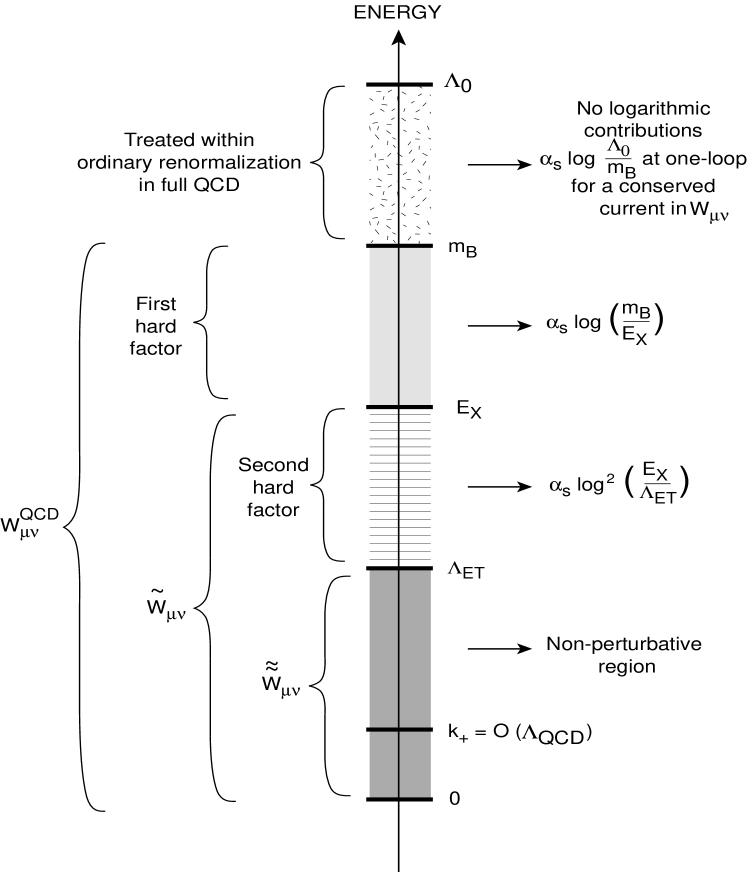
Figure 1: Pictorial description of factorization in the effective theory.

In fig. 1, we give a pictorial description of the above procedure.

4 OPE

The amplitude for the decay (7), which we take as our example from now on, can be written at the lowest order in the weak coupling as

$$A=\frac{G_{F}}{\sqrt{2}}\,\langle l\nu\mid L_{\mu}\mid 0\rangle\,\langle X|J^{\mu}|B\rangle,$$ (42)

where $L_{\mu}$ is the leptonic current and $J_{\mu}$ is the hadronic one:

$$J_{\mu}(x)\equiv\overline{q}(x)\Gamma_{\mu}b(x)$$ (43)

with $\Gamma_{\mu}=\gamma_{\mu}(1-\gamma_{5})$, $q(x)$ a light quark field and $b(x)$ the beauty quark field. Taking the square of (42) and summing over the final states, we arrive at the hadronic tensor defined in eq. (8). By the optical theorem, we can relate the hadronic tensor $W_{\mu\nu}$ to the imaginary part of the Green function or forward hadronic tensor $T_{\mu\nu}$:

$$W_{\mu\nu}=-\frac{1}{\pi}{\rm Im}\,\,T_{\mu\nu},$$ (44)

where

$$T_{\mu\nu}\ \equiv-i\int d^{4}x\,e^{-iqx}\langle B|T\left(J_{\mu}^{\dagger}(x)J_{\nu}(0)\right)|B\rangle.$$ (45)

4.1 The HQET

We are interested in the evaluation of $T_{\mu\nu}$ in the effective theory and we discuss in this section the first factorization step: replacing the beauty quark by a quark in the HQET. As is well known, we can decompose the heavy quark field $b(x)$ into two effective quark and antiquark fields $h_{v}$ and $H_{v}$ 

$$b(x)=e^{-im_{B}v\cdot x}\left[h_{v}(x)+H_{v}(x)\right],$$ (46)

satisfying

$$P_{+}\ h_{v}=h_{v},\ \ P_{-}\ h_{v}=0,\ \ \ P_{-}\ H_{v}=H_{v},\ \ P_{+}\ H_{v}=0,$$ (47)

where $P_{\pm}=(1\pm\hat{v})/2$ are the projectors over the components with positive and negative energies, respectively. The field $H_{v}$ is neglected (which amounts to neglecting heavy-pair creation), so that

$$b(x)\simeq e^{-im_{B}v\cdot x}\ h_{v}(x).$$ (48)

By using eq. (48) we obtain

$$\widetilde{T}_{\mu\nu}=-i\int d^{4}x\ e^{iQ\cdot x}\langle B(v)|T\ \bar{h}_{v}(x)\Gamma_{\mu}^{\dagger}\ q(x)\ \bar{q}(0)\Gamma_{\nu}\ h_{v}(0)|B(v)\rangle.$$ (49)

We now use the Wick theorem and we single out the only contraction that is relevant to $B$ decay:

$$\widetilde{T}_{\mu\nu}=\int d^{4}x\ e^{iQx}\langle B|\bar{h}_{v}(x)\Gamma_{\mu}^{\dagger}\,S(x|0)\Gamma_{\nu}h_{v}(0)|B\rangle,$$ (50)

where $S(x|0)$ is the light quark propagator. Note that the operator entering the right-hand side of eq. (50) is already normal ordered, since $h_{v}$ has only the component that annihilates heavy quarks, while $\bar{h}_{v}$ only the components that create them. We can express the Fourier transform of the light quark propagator as

$$S(Q+iD)=\frac{1}{i\hat{D}+\hat{Q}+i0}=\frac{i\hat{D}+\hat{Q}}{Q^{2}+2iD\cdot Q-D^{2}-g/2\ \sigma_{\mu\nu}G^{\mu\nu}+i0}$$ (51)

where $\sigma_{\mu\nu}\equiv i/2[\gamma_{\mu},\gamma_{\nu}]$ is a generator of the Lorentz group, $G_{\mu\nu}\equiv-i/g[D_{\mu},D_{\nu}]$ is the field strength and $D_{\mu}\equiv\partial_{\mu}-igA_{\mu}$ is the covariant derivative. In eq. (51), $0$ denotes, as usual, an infinitesimal positive number and gives the prescription to deal with pole or branch-cut singularities. There are three different regions according to the value of the jet invariant mass, which are described by three different full or effective theories:

$$i)\qquad m_{X}^{2} \sim O(E_{X}^{2}),$$

$$ii)\qquad m_{X}^{2} \sim O(\Lambda_{QCD}^{2}\,),$$

$$iii)\qquad m_{X}^{2} \sim O(\Lambda_{QCD}\,E_{X}).$$ (52)

Since the derivative of the rescaled $h_{v}$ field brings down the residual momentum $k^{\prime}$, and it is therefore an operator with matrix elements of order $O\left(\Lambda_{QCD}\right)$, the matrix elements of the operators entering the light quark propagator have a size of the order of

$$\langle\,i\hat{D}\,\rangle \sim O(\Lambda_{QCD}),$$

$$\langle\,2iD\cdot Q\ \rangle \sim O(\Lambda_{QCD}\,E_{X}),$$

$$\langle\,D^{2}\,\rangle \sim O(\Lambda_{QCD}^{2}),$$

$$\langle\,\sigma_{\mu\nu}G^{\mu\nu}\,\rangle \sim O(\Lambda_{QCD}^{2}).$$ (53)

Let us discuss these regions in turn in the next section.

4.2 General kinematical regions

$i)$

This region corresponds to a jet $X$ with a large invariant mass, of the order of the energy:

$$m_{X}\sim O\left(E_{X}\right)\,.$$ (54)

To a first approximation all the covariant derivative terms can be neglected, so that

$$S(Q+iD)\ \simeq\ \frac{\hat{Q}}{Q^{2}+i0},$$ (55)

i.e. the light quark can be described as a free quark. A higher accuracy is reached when expanding the propagator in powers of the covariant derivative operators up to the required order. We have here an application of the $1/m_{B}$ expansion up to a prescribed (finite) order . In this region there are no large adimensional ratios of scales, the latter being all of the same order. This implies that in perturbation theory we do not hit large logarithmic corrections to be resummed to all orders in $\alpha_{S}.$ This region is not relevant to the endpoint electron spectrum because the hadronic jets takes away most of the available energy. This region will not be discussed further here.

$ii)$

This region involves a recoiling hadronic system with a mass of the order of the hadronic one: it can be a single hadron or very few hadrons. The dynamics is dominated by the emission, with consequent decay, of few resonances; it is a completely non-perturbative problem. According to the estimates (53), no term can be neglected in the light quark propagator. We are faced with full QCD dynamics as far as the final hadronic state is concerned. This region must be evaluated by an explicit sum over all the kinematically possible hadronic states, and the latter have to be computed with a non-perturbative technique such as a quark model or lattice QCD. This region will not be discussed here either.

$iii)$

This region is intermediate between $i)$ and $ii)$ and as such it has both perturbative and non-perturbative components. Roughly speaking, we have to take into account non-perturbative effects for the initial state hadron, while we can neglect final state binding effects. This region is characterized by a small ratio of the jet invariant mass to the jet energy, and thus involves the large adimensional ratio in (3). As always is the case, perturbation theory generates logarithms of the above adimensional ratio, eq. (26). The term $2\,iD\cdot Q$ at the denominator cannot be brought at the numerator (with a truncated operatorial expansion) because it is of the same order as $m_{X}^{2}.$ At lowest order, the other covariant derivative terms can be neglected, to give:

$$S(Q+iD)\simeq\frac{\hat{Q}}{m_{X}^{2}+2iD\cdot Q+i0}.$$ (56)

One can reach a higher level of accurary keeping these latter corrections up to a given order. The rest of the paper deals with region $iii)$ at the lowest order in $1/m_{B}$.

4.3 The LEET

In this section we discuss the second factorization step, which involves the description of the final $up$ quark in the LEET, according to eq. (56). Let us define the adimensional vector $n_{\mu}$ as:

$$n_{\mu}=\frac{Q_{\mu}}{Q\cdot v}~{}.$$ (57)

This $n_{\mu}$ has a normalized time component, $n_{0}=1$. In the “semi-inclusive” endpoint region $iii)$:

$$n^{2}~{} = \frac{m_{X}^{2}}{E_{X}^{2}}$$ (58)

$$= O\left(\frac{\Lambda_{QCD}}{E_{X}}\right)~{}\ll 1.$$

We will show later that $n$ can be replaced by a vector lying exactly on the light-cone, i.e.

$$n\rightarrow\overline{n},$$ (59)

where $\overline{n}^{\mu}=(1;0,0,-1)$ ( $\overline{n}^{\,2}=0$), representing the direction of the hadronic jet, the $-z$ axis. We can write

$$S(Q+iD)=\frac{1}{2v\cdot Q}\;\ \frac{\hat{Q}}{iD_{+}-k_{+}+i0},$$ (60)

where $k_{+}$ has been defined in eq. (22) and $D_{+}\equiv\overline{n}\cdot D.$ We can simplify the tensor structure of $T_{\mu\nu}$ by using the identity

$$\bar{h}_{v}\Gamma_{\mu}h_{v}=\frac{1}{2}{\rm Tr}(\Gamma_{\mu}P_{+})\ \bar{h}_{v}h_{v}-\frac{1}{2}{\rm Tr}(\gamma_{\mu}\gamma_{5}P_{+}\Gamma_{\mu}P_{+})\,\bar{h}_{v}\gamma^{\mu}\gamma_{5}h_{v},$$ (61)

which is valid for any $\Gamma_{\mu}$. The matrix element of the axial vector current between the $B$-meson states vanishes by parity invariance, so that :

$$\widetilde{\widetilde{T}}_{\mu\nu}=\;s_{\mu\nu}\;\frac{1}{2v\cdot Q}\ F(k_{+}),$$ (62)

where we have defined the “light-cone” function

$$F(k_{+})\equiv\langle B(v)\mid h_{v}^{\dagger}\frac{1}{iD_{+}-k_{+}+i0}h_{v}\mid B(v)\rangle,$$ (63)

and

$$s_{\mu\nu}\equiv\frac{1}{2}\,{\rm Tr}\left[\Gamma_{\mu}^{\dagger}\hat{Q}\Gamma_{\nu}P_{+}\right]\;$$ (64)

is the “spin factor”, containg the leading spin effects. The factor $1/(2v\cdot Q)$ is a jacobian, which appears as we go from the full QCD variable $Q^{2}$ to the effective theory variable $k_{+}.$

Taking the imaginary part of $T_{\mu\nu}$, we obtain (see relation (44)):

$$\widetilde{\widetilde{W}}_{\mu\nu}=\;s_{\mu\nu}\;\frac{1}{2v\cdot Q}\ f(k_{+}),$$ (65)

where

$$f(k_{+})\equiv-\frac{1}{\pi}{\rm Im}\,F(k_{+})$$ (66)

is the shape function. By using the formula

$$\frac{1}{iD_{+}-k_{+}+i0}={\rm P}\frac{1}{i\,D_{+}-k_{+}}-i\pi\,\delta(iD_{+}-k_{+}),$$ (67)

we recover the definition of the shape function given by eq. (10). Note that it involves the non-local operator $h_{v}^{\dagger}\,\delta(k_{+}-iD_{+})\,h_{v}$, which results from the resummation of the towers of operators of the form $\left(Q\cdot D\right)^{n}$.

4.4 The Variable Mass

The hadronic tensor can be written in the effective theory in terms of the shape function as:

$$\widetilde{\widetilde{W}}_{\mu\nu}=\ s_{\mu\nu}\int_{-\infty}^{0}dk_{+}\ \delta\left(Q^{2}+2k_{+}v\cdot Q\right)\,f(k_{+});$$ (68)

in the second member, $k_{+}$ is an integration, i.e. dummy, variable. In the free theory, with an on-shell $b$-quark (i.e. $k^{\prime}=0$ in eq. (16)),

$$f^{0}(k_{+})=\delta(k_{+}-0),$$ (69)

so that

$$W_{\mu\nu}^{0}=s_{\mu\nu}\ \delta(Q^{2}-0).$$ (70)

The hadronic tensor can be written, up to terms of order $k_{+}^{2}\sim O\left(\Lambda_{QCD}^{2}\right),$ as

$$\widetilde{\widetilde{W}}_{\mu\nu}=\ s_{\mu\nu}(Q)\int dm_{\ast}\ \delta\left(Q_{\ast}^{2}-0\right)\,f(m_{\ast}-m_{B}),$$ (71)

where we have defined

$$Q_{\ast}\equiv m_{\ast}v-q$$ (72)

and $m_{\ast}$ is the “variable” or “fragmentation” mass, defined in eq.(11). Since $m_{\ast}$ is just a shift of $k_{+}$, the range is

$$-\infty<m_{\ast}\leq m_{B}.$$ (73)

Inside $s_{\mu\nu}$ we can replace $Q$ with $Q_{\ast},$ because that amounts only to a correction of order $k_{+}=O(\Lambda_{QCD})$, so that

$$\widetilde{\widetilde{W}}_{\mu\nu}(v,Q)=\ \int_{0}^{m_{B}}dm_{\ast}\ \varphi(m_{\ast})\,\ W_{\mu\nu}^{0}(v,Q_{\ast}),$$ (74)

where

$$W_{\mu\nu}^{0}(v,Q^{\ast})=\ s_{\mu\nu}(Q_{\ast})\ \delta\left(Q_{\ast}^{2}-0\right)$$ (75)

is the hadronic tensor in the free theory for a heavy quark of mass $m_{\ast}$ and

$$\varphi(m_{\ast})\equiv f(m_{\ast}-m_{B})$$ (76)

is the distribution for the effective mass $m_{\ast}$ of the $b$-quark inside the $B$-meson at disintegration time. Equation (74) is the fundamental result of factorization in semi-inclusive heavy flavour decays: it says that the hadronic tensor in the effective theory can be expressed as the convolution of the hadronic tensor in the free theory with a variable mass times a distribution probability for this mass. That offers also the physical interpretation to the shape function anticipated in the introduction: it represents the probability that the $b$ quark has an effective mass $m_{\ast}$ at the decay time. Since this tensor encodes all the hadron dynamics, $any$ distribution can be expressed in a similar factorized form.

5 Factorization in the quantum theory

In this section we discuss factorization in the quantum theory, i.e. the separation of short-distance and long-distance contributions, including loop effects.

A shape function $f(k_{+})^{QCD}$ and a light-cone function $F(k_{+})^{QCD}$ can also be defined in full QCD by means of the relations [10]:

$$T_{\mu\nu}^{QCD}\equiv\left(s_{\mu\nu}\;+\Delta s_{\mu\nu}\right)\frac{1}{2v\cdot Q}\ F(k_{+})^{QCD}$$

and

$$W_{\mu\nu}^{QCD}\equiv\left(s_{\mu\nu}\;+\Delta s_{\mu\nu}^{\prime}\right)\frac{1}{2v\cdot Q}\ f(k_{+})^{QCD},$$

where $\Delta s_{\mu\nu}$ and $\Delta s_{\mu\nu}^{\prime}$ are defined as the part of the spin structure not proportional to $s_{\mu\nu}$. The tensors $\Delta s_{\mu\nu}$ and $\Delta s_{\mu\nu}^{\prime}$ represent residual spin effects not described by the effective theory (ET), which do not contribute to the Double-Logarithmic Approximation (DLA). In DLA the forward tensor can therefore be written as

$$T_{\mu\nu}^{QCD}=\;s_{\mu\nu}\;\frac{1}{2v\cdot Q}\ F(k_{+})^{QCD},$$ (77)

where the “light-cone function” is given by

$$F(k_{+})^{QCD}\equiv\frac{1}{-k_{+}+i0}\left[1+a\,C\right],$$ (78)

$a\equiv\alpha_{S}$

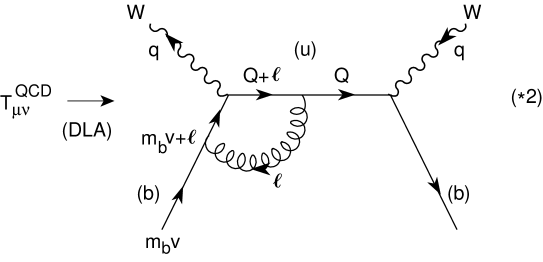
Figure 2: Vertex corrections to the light-cone function $F^{QCD}(k_{+})$

$C_{F}/\pi$ and $C$ is the scalar triangle diagram (see fig. 2):

$$C\equiv\ -i\,v\cdot Q\int\frac{d^{4}l}{\pi^{2}}\ \frac{1}{(l+Q)^{2}+i0}~{}\ \frac{1}{v\cdot l+l^{2}/2m+i0}~{}\ \frac{1}{l^{2}+i0}.$$ (79)

We have set the light quark mass equal to zero [21].

The hadronic tensor relevant to the decay is obtained by taking the imaginary part according to eq. (44). This transforms the products in convolutions, which are converted again into ordinary products by the well-known Mellin transform [22].

Infrared singularities (soft & collinear) are regulated by the virtuality $Q^{2}\neq 0$ of the external $up$ quark. We may write

$$Q^{\mu}\cong E_{X}\left(1+\frac{n^{2}}{4};0,0,-1+\frac{n^{2}}{4}\right)=E_{X}\,\left(v_{-}+\frac{n^{2}}{4}v_{+}\right)$$ (80)

and

$$n^{\mu}\cong v_{-}^{\mu}+\frac{n^{2}}{4}v_{+}^{\mu}\,,\qquad\overline{n}^{\,\mu}=v_{-}^{\mu}$$ (81)

where we defined the light-cone versors

$$v_{+}\equiv\left(1;0,0,1\right),\qquad v_{-}\equiv\left(1;0,0,-1\right).$$ (82)

Let us now consider the properties of the integral $C$. First, it is adimensional. Second, it is UV-finite for power counting: the integrand has three ordinary scalar propagators with a total of six powers of momentum at the denominator. This implies that $C$ does not depend on an ultraviolet cutoff $\Lambda_{UV}$ as long as it is larger than any physical scale of the process, namely

$$\Lambda_{UV}\gg m_{B}.$$ (83)

Third, as already discussed, $C$ is also IR-finite as long as $Q^{2}\neq 0.$ For $Q^{2}>0$ there is an imaginary part, related to the propagation of the real $up$ and gluon pair, while for $Q^{2}<0$ the integral is real. Therefore $C$ does depend on adimensional ratios of three different scales: $m_{B},E_{X}$ and $m_{X}.$ There are only two independent ratios, which we choose as $m_{B}/E_{X}$ and$\,\,m_{X}/E_{X}.$ We are going to decompose the integral $C$ in a sum of various integrals; at the end, one of them will correspond to the double-logarithmic contribution to the shape function $f(k_{+})$ in the low-energy ET. The other integrals represent additional contributions and they are mostly short-distance dominated in lattice-like regularizations. This decomposition consists of two separate steps, which will be described in the following sections.

5.1 From QCD to HQET

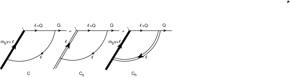
Figure 3: First decomposition in $T_{\mu\nu}$. The thick, thin and double lines represent the massive quadratic, massless quadratic and time-like eikonal propagators, respectively.

In the first step we isolate a hard factor by simply subtracting and adding back the integral with the full beauty quark propagator replaced by a static one (see fig. 3)

$$C=C_{s}+C_{h},$$ (84)

where

$$C_{s}\equiv-iv\cdot Q\int\frac{d^{4}l}{\pi^{2}}\ \frac{1}{(l+Q)^{2}+i0}~{}\ \frac{1}{v\cdot l+i0}~{}\ \frac{1}{l^{2}+i0},$$ (85)

and

$$C_{h}\equiv i\frac{v\cdot Q}{2m}\int\frac{d^{4}l}{\pi^{2}}\ \frac{1}{(l+Q)^{2}+i0}\ \frac{1}{v\cdot l+i0}\,\frac{1}{v\cdot l+l^{2}/2m+i0}.$$ (86)

The above decomposition parallels that one performed in section 4 in operatorial language. The light-cone function factorizes at order $\alpha_{S}$ according to

$$F(k_{+})^{QCD}=\frac{1}{-k_{+}+i0}\left[1+a\,C\right]=\frac{1}{-k_{+}+i0}\left[1+a\,C_{h}\right]\left[1+a\,C_{s}\right].$$ (87)

We expect that $C_{s}$ has the same infrared behaviour as $C$; it will be subjected to a further decomposition in the next sections; $C_{h}$  is the “hard factor”, i.e. the difference between QCD and the static limit for the $b$ quark. The latter integral is both UV- and IR-finite. The ultraviolet finiteness stems from power counting: the integrand has two scalar propagators and a static propagator with a total of five powers of momentum in the denominator . In the infrared region, all the components of the loop momentum are small

$${\rm IR}:\quad l_{\mu}\rightarrow\rho l_{\mu},\quad\rho\rightarrow 0,$$ (88)

so we can neglect the terms that are quadratic in $l^{\mu}$ in the propagator denominators:

$$C_{h\,,IR}\sim\int d^{4}l\frac{1}{2l\cdot Q+Q^{2}+i0}~{}~{}\ \frac{1}{(v\cdot l+i0)^{2}}.$$ (89)

Integrating over $l_{0}$, and closing the contour in the upper half of the $l_{0}$-plane, we see that there are no enclosed poles and the integral vanishes (QED). Inside $C_{h}$ we can therefore make the replacement 

$$Q^{\mu}\quad\rightarrow\quad\overline{Q}^{\,\mu}\equiv E_{X}\,v_{-}\qquad\qquad(\overline{Q}^{\,2}=0).$$ (90)

It follows that $C_{h}$ depends only on $m_{B}$ and $E_{X}$: $C_{h}=C_{h}(m_{B},E_{X}).$ Since it is adimensional, it may depend only on the adimensional hadronic energy

$$z\equiv\frac{2E_{X}}{m_{B}},$$ (91)

i.e. $C_{h}=C_{h}(z).$ An explicit computation gives

$$C_{h}=\log\left(1-z\right)\log z+Li_{2}(z)\simeq-z\log z\quad\left(z\ll 1\right),$$ (92)

$C_{h}$ does not contain large logarithmic contributions in the limit $z\rightarrow 0$, i.e. $\log z$ terms . This is related to the fact that $C_{h}$ and $C_{s}$ are UV-convergent. In general, single logarithms of the hadronic energy, $\log z,$ do appear, representing the difference between the interaction of a full propagating heavy quark, of mass $m_{B},$ and that one of a static quark. The relevant interaction energies are between the beauty mass $m_{B}$ and the hadronic energy $E_{X}$,

$$\alpha_{S}\,\int_{z^{2}m_{B}^{2}}^{m_{B}^{2}}\frac{dk^{2}}{k^{2}}=-2\,\alpha_{S}\,\log z.$$ (94)

The logarithms (94) are resummed, as usual, by replacing the bare coupling with the running coupling and exponentiating, so that the above formula is corrected into:

$$1+\gamma_{0}\alpha_{S}\int_{z^{2}m_{B}^{2}}^{m_{B}^{2}}\frac{dk^{2}}{k^{2}}\quad \rightarrow \quad\exp\left[\gamma_{0}\int_{z^{2}m_{B}^{2}}^{m_{B}^{2}}\frac{dk^{2}}{k^{2}}\,\alpha_{S}(k^{2})\right]$$ (95)

$$= \exp\left[-2\,\alpha_{S}\gamma_{0}\log z+2\gamma_{0}\beta_{0}\,\alpha_{S}^{2}\,\log^{2}z+\cdots\right],\quad$$

where $\beta_{0}\equiv 1/(4\pi)(11/3\,N_{c}-2/3\,n_{f})$ and $\alpha_{S}\equiv\alpha_{S}(m_{B})$.

Let us summarize the above discussion. A first coefficient function is introduced, which takes into account the fluctuations with energy $\varepsilon$ in the range

$$E_{X}<\varepsilon<m_{B}.$$ (96)

In the language of Wilson’s renormalization group, we are lowering the UV cutoff of the effective hamiltonian from $m_{B}$ to $E_{X}$.

5.2 Infrared factorization

The second factorization step involves the separation of the various infrared contributions to the process, one of which will ultimately lead to the shape function. This step forces us to introduce explicitly an ultraviolet cutoff $\Lambda$ from which the various factors depend separately. In other words, the decomposition of $C_{s}$ introduces fictitious UV divergences, which cancel in the sum. As anticipated in the overview section, infrared factorization in our scheme involves two different operations:

• the separation of the various pole contributions to the QCD amplitude according to the Cauchy theorem;

• the lowering of the UV cutoff from $\Lambda_{UV}\gtrsim E_{X}$ to $\Lambda_{UV}=\Lambda_{ET}\ll E_{X},$where $\Lambda_{ET}$ is the cutoff of the final low-energy effective theory, in which the shape function is defined (the latter contains the majority of the non-perturbative effects).

Step 1) will be discussed in this section, while step 2) is treated mostly in the next section.

$C_{s}$ is UV-convergent, as is clear again from power counting, and it does not depend on the beauty mass $m_{B}$, which has been sent to infinity, so that $C_{s}=C_{s}(E_{X},m_{X}).$ The only adimensional variable that can be constructed out of $E_{X}$ and $m_{X}$ is their ratio or, equivalently, $n^{2}$ (see eq. (58)). Since $C_{s}$ is adimensional it may depend only on $n^{2}$: $C_{s}=C_{s}(n^{2}).$ The explicit computation in DLA gives

$$C_{s}=-\frac{1}{2}\log^{2}(-n^{2}-i0)\qquad\quad\quad\quad\left(DLA\right).$$ (97)

The infrared factorization is performed by integrating $C_{s}$ over the energy $l_{0}$ using the Cauchy theorem. There are three poles in the lower half of the $l_{0}$-plane related to the propagation of a real static quark, a real gluon and a real $up$ quark, located respectively at

$$l_{0}=-i0,\qquad l_{0}=+|\overrightarrow{l}|-i0,\qquad l_{0}=-Q_{0}+\sqrt{(Q_{3}+l_{3})^{2}+l_{\bot}^{2}}-i0.$$ (98)

In the upper half-plane, instead, there are only two poles, related to the gluon and the up propagator:

$$l_{0}=-|\overrightarrow{l}|+i0,\qquad l_{0}=-Q_{0}-\sqrt{(Q_{3}+l_{3})^{2}+l_{\bot}^{2}}+i0$$ (99)

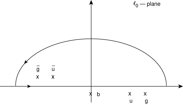
Figure 4: Poles of $C_{s}$ in the $l_{0}$-plane. The crosses labelled by $b$, $u$ and $g$ represent the particle poles in the static beauty, $up$ and gluon propagators, respectively. The crosses labelled by $\bar{u}$ and $\bar{g}$, instead, represent the antiparticle poles in the $up$-quark and gluon propagators.

The poles in (99) are conventionally related to a propagation that goes backward in time; they will therefore be called the antiparticle poles. We close for simplicity the integration contour in the upper half-plane and we have two residue contributions related to the antigluon pole ad the anti-$up$ pole respectively (see fig.4):

$$C_{s}=C_{g}+C_{q}.$$ (100)

The antigluon and the anti-$up$ contributions are given respectively by

$$C_{g} = \frac{2}{\pi}v\cdot Q\int d^{3}l~{}\ \left.\ \frac{1}{l_{0}-|\overrightarrow{l}|+i0}\,\frac{1}{v\cdot l+i0}\frac{1}{Q^{2}+2l\cdot Q+i0}\right|_{l_{0}=-|\overrightarrow{l}|+i0}$$ (101)

$$C_{q} = \ \frac{2}{\pi}v\cdot Q\int d^{3}l\ \left.\frac{1}{l_{0}+Q_{0}-|\overrightarrow{l}+\overrightarrow{Q}|+i0}\frac{1}{v\cdot l+i0}\frac{1}{l^{2}+i0}\right|_{l_{0}=-Q_{0}-\sqrt{(Q_{3}+l_{3})^{2}+l_{\bot}^{2}}+i0}$$

As we see by power counting, $C_{g}$ and $C_{q}$ are UV-divergent and it is therefore necessary to introduce an ultraviolet regularization to treat them separately.

The light-cone function factorizes after this second step as

$$F(k_{+})^{QCD}=\frac{1}{-k_{+}+i0}\left[1+a\,C_{h}\right]\left[1+a\,C_{q}\right]\left[1+a\,C_{g}\right],$$ (102)

i.e. as a product of three factors.

5.2.1 Wilson line representation

Before explicitly computing these 3-dimensional integrals, let us represent them as 4-dimensional ones, i.e. as one-loop integrals of a properly chosen field theory:

$$C_{g}\equiv-iv\cdot Q\int\frac{d^{4}l}{\pi^{2}}\ \frac{1}{Q^{2}+2l\cdot Q+i0}~{}\ \frac{1}{v\cdot l+i0}~{}\ \frac{1}{l^{2}+i0}$$ (103)

and

$$C_{q}\equiv iv\cdot Q\int\frac{d^{4}l}{\pi^{2}}\ \frac{1}{(l+Q)^{2}+i0}~{}\ \frac{1}{v\cdot l+i0}~{}\ \frac{1}{Q^{2}+2l\cdot Q+i0}$$ (104)

The proof of the above equations is just by integration over $l_{0}$: closing the integration contour in the upper half-plane of $l_{0}$, we enclose a single pole, whose residue gives the 3-dimensional integrals in eqs. (101); $C_{g}$ and $C_{q}$ involve one full - i.e. quadratic - propagator and two eikonal - i.e. linear - propagators. It is easy to check that the algebraic sum of $C_{g}$ and $C_{q}$ in the above expressions reproduces the integral $C_{s}$ defined in eq. (85). Introducing the variable $k_{+}$, the integral $C_{g}$ can be written in the “familiar” form

$$C_{g}(k_{+})\equiv\frac{-i}{2}\int\frac{d^{4}l}{\pi^{2}}\ \frac{1}{-k_{+}+l\cdot n+i0}~{}\ \frac{1}{v\cdot l+i0}~{}\ \frac{1}{l^{2}+i0}.$$ (105)

The geometrical interpretation is the following: $C_{g}(k_{+})$ is the one-loop correction to a vertex composed of an on-shell Wilson line along the time axis, and a Wilson line along the direction $n$ off-shell by $k_{+}$. Note that

$$l\cdot n=l_{+}+\frac{n^{2}}{4}l_{-},$$ (106)

so that eq. (105) represents the vertex correction in Feynman gauge to the function

$$F(k_{+})_{n^{2}\neq 0}\equiv\langle B(v)\mid h_{v}^{\dagger}\frac{1}{iD_{+}+in^{2}/4D_{-}-k_{+}+i0}h_{v}\mid B(v)\rangle.$$ (107)

The imaginary part of the above function equals $-1/\pi$ times the shape function off the light-cone, $n^{2}\neq 0$:

$$f(k_{+})_{n^{2}\neq 0}\equiv\langle B(v)\mid h_{v}^{\dagger}\,\delta\left(k_{+}-iD_{+}-in^{2}/4D_{-}\right)\,h_{v}\mid B(v)\rangle.$$ (108)

In the limit $n^{2}\rightarrow 0$ (see section 6) we recover the correction to the light-cone function $F(k_{+})$, which was computed in ref.  [8, 9, 10].

We can give a similar description for $C_{q}$. The 4-dimensional representation for $C_{q}$ involves an on-shell Wilson line along the time direction, a Wilson line along the direction $n$ off-shell by $k_{+}$, and a light quark propagator with momentum $l+Q$

$$C_{q}\equiv\frac{i}{2}\int\frac{d^{4}l}{\pi^{2}}\ \frac{1}{-k_{+}+l\cdot n+i0}~{}\ \frac{1}{v\cdot l+i0}\,\,\frac{1}{(l+Q)^{2}+i0}.$$ (109)

Note that the expressions for $C_{g}$ and $C_{q}$ are very similar: they differ by an overall sign and by the replacement in the quadratic propagator of $l\rightarrow l+Q$. For future reference, let us note that the latter shift involves only the zero and the third components of $l$, not the transverse ones.

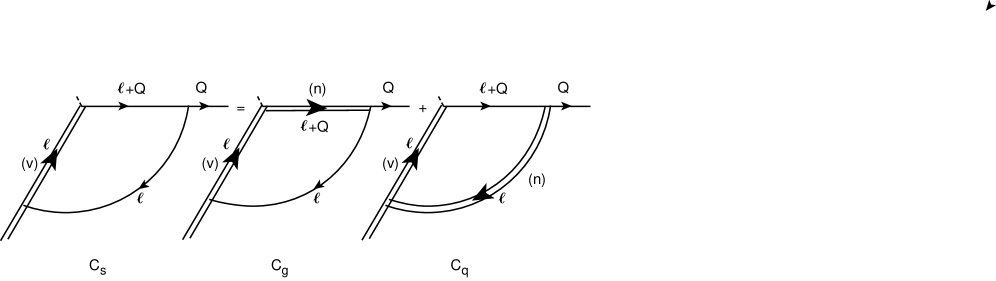
Figure 5: Second decomposition in $T_{\mu\nu}$. The thin and double lines represent the massless quadratic and eikonal propagators, respectively. The symbols (v) and (n) indicate that the eikonal propagators must be taken along the directions $v$ and $n$.

In fig.5 the decomposition of $C_{s}$ into $C_{g}$ and $C_{q}$ is represented.

5.2.2 Space Momenta Cutoff

We consider the bare theory with the regularization introduced in ref. [10]: a sharp cutoff on the spatial loop momenta $\Lambda_{S}$ (see next section). Integrating $C_{g}$ over $l_{0}$ by closing the integration contour upward and integrating over the azimuthal angle, we obtain

$$C_{g}=-\int_{0}^{\Lambda_{S}}dl\int_{-1}^{1}d\cos\theta\frac{1}{k_{+}+l\left(1-\cos\theta\right)+n^{2}l/4\left(1+\cos\theta\right)},$$ (110)

where we have used the definition of $Q^{\mu}$ in eq. (80) and $l\equiv|\overrightarrow{l}|$. Integrating over the polar angle, we obtain

$$C_{g}=-\int_{0}^{2\Lambda_{S}}\frac{dl}{l}\log\left[\frac{k_{+}+l}{k_{+}+n^{2}\,l/4}\right].$$ (111)

Assuming a cutoff much larger than any physical scale in the process, i.e.

$$\Lambda_{S}\gg E_{X},$$ (112)

we obtain in DLA

$$C_{g}=-\frac{1}{2}\log^{2}\frac{E_{X}}{k_{+}-i0}-\log\frac{\Lambda_{S}}{E_{X}}\log\frac{E_{X}}{-k_{+}+i0}.$$ (113)

Three scales enter in $C_{g}$: $k_{+},\,\Lambda_{S}$ and $E_{X}.$ The appearance of $k_{+}$ and the cutoff $\Lambda_{S}$ was expected, because these two quantities represent the infrared and the ultraviolet scale, respectively. The noticeable fact is that also the hadronic energy $E_{X}$ makes its appearance. $C_{g}$ contains a double-logarithm of the infrared kinematical scale $k_{+}$ (related to the overlap of the soft and the collinear region, which extends up to $\Lambda_{S}$); it also contains a single logarithm of the cutoff. The appearance of the hadronic energy $E_{X}$ comes from the necessity of a third mass scale for the function $C_{g}$, which behaves like $\log^{2}k_{+}$ in $k_{+}$ and like $\log\Lambda_{S}$ in $\Lambda_{S}.$

When $l\gg E_{X}$ the integrand behaves as

$$-\frac{1}{l}\log\left[\frac{k_{+}+l}{k_{+}+n^{2}\,l/4}\right]\sim\frac{1}{l}\log\frac{n^{2}}{4}$$ (114)

and produces a single-logarithmic ultraviolet divergence. As eq. (114) clearly indicates, $n^{2}\neq 0$ regulates the collinear or light-cone singularity: up to now we have indeed taken kinematics into account exactly together with a large cutoff. It is interesting to note that if we take a cutoff much smaller than the hadronic energy (as we will do in the “final” low-energy effective theory),

$$\Lambda_{ET}\,\ll\,E_{X},$$ (115)

we have

$$n^{2}\,l\,\leq\,\frac{m_{X}^{2}}{E_{X}^{2}}\,\,\Lambda_{ET}\,\ll\,k_{+},$$ (116)

and $C_{g}$ simplifies in

$$C_{g}\left(\Lambda_{ET}\right)\simeq-\int_{0}^{2\Lambda_{ET}}\frac{dl}{l}\log\left(\frac{k_{+}+l}{k_{+}}\right).$$ (117)

The quantity $n^{2}$ does not enter anymore and the integrand is the same as that with the approximate light-cone kinematics $n^{2}=0$, i.e. with $n$ replaced by $\overline{n}$. The physical explanation is that soft gluons are not able to distinguish between the two slightly different directions $n$ and $\overline{n}$. Formally, with the small cutoff (115) we can take the limit (6) inside the integral. In other words, in the low-energy effective theory, we effectively are always in the light-cone limit. For $l\gg k_{+}$, the integrand in eq. (117) has the asymptotic behaviour

$$\frac{1}{l}\log\frac{l}{k_{+}},$$ (118)

implying a double-logarithmic behaviour with respect to $\Lambda_{ET}$ upon integration over $l$, in contrast with the single logarithmic behaviour of the integrand in (114). These properties will be studied systematically in the next section, in which we consider the effective theory on the light-cone.

For the computation of $C_{q}$, it is convenient to first make the shift $l\rightarrow l-Q$ in the expression of $C_{q},$ eq. (104), and then to compute the residue of the light quark pole at $l_{0}=-|\overrightarrow{l}|+i0$: this is legitimate if condition (112) holds. We find

$$C_{q}=\log\frac{\Lambda_{S}}{E_{X}}\log\frac{E_{X}}{-k_{+}+i0}\quad\quad\quad(\Lambda_{S}\gg E_{X}).$$ (119)

The three scales appearing in $C_{g}$ do appear also in $C_{q}$. We note that $C_{q}$ contains a single logarithm of $k_{+}$, i.e. it is subleading by one logarithm in the infrared counting with respect to $C_{g}$. It has a single-logarithmic UV divergence.

If we compute the integral in eq. (104) with a small cutoff (115), we do not find any infrared logarithm, in contrast with what happens instead with $C_{g}$. Thus the logarithmic contributions to $C_{q}$ come from high-energy gluons and that is an indication that $C_{q}$, unlike $C_{g}$, is short-distance dominated.

One can check that the correct value of $C_{s}$ is reproduced by summing $C_{g}$ and $C_{q}$; in particular, UV divergences cancel.

At the level of logarithmic accuracy, we can replace the strong inequality (112) with a weaker one:

$$\Lambda_{S}\geq E_{X}.$$ (120)

Setting in particular

$$\Lambda_{S}=E_{X},$$ (121)

the expressions for the gluon and quark-pole residue read

$$C_{g}\left(\Lambda_{S}=E_{X}\right) = -\frac{1}{2}\log^{2}\frac{E_{X}}{k_{+}-i\epsilon}=C_{s},$$

$$C_{q}\left(\Lambda_{S}=E_{X}\right) = 0,$$ (122)

i.e. the gluon-pole term gives the whole contribution while the quark-pole factor vanishes. The term $C_{q}$ therefore has the role of correcting $C_{g}$ when $\Lambda_{S}\neq E_{X}.$

Since ultraviolet singularities are single-logarithmic for a large cutoff (eqs. (113) and (119)), other regularizations such as DR give similar results. In other words, the regularization scheme dependence is the usual one: the logarithmic term in the one-loop amplitude is scheme independent while the finite part is scheme dependent.

6 The effective theory on the light-cone, the LEET

In full QCD infrared singularities are regulated by the unique quantity $m_{X}^{2}\neq 0$. In the effective theory, the light quark propagator is replaced by an eikonal one

$$\frac{1}{\left(l+Q\right)^{2}+i0}=\frac{1}{Q^{2}+2l\cdot Q+l^{2}+i0}\,\,\rightarrow\,\,\frac{1}{Q^{2}+2l\cdot Q+i0}.$$ (123)

In the expression on the right-hand side $l^{2}$ has been neglected and as a consequence $Q_{\mu}$ enters in two distinct and independent ways: its square $Q^{2}$ represents the virtuality of the eikonal line at $l_{\mu}=0$, while its components $Q^{\mu}$ are the coefficients of the linear combination of the loop-momentum components $l_{\mu}$ in the term $2\,l_{\mu}\,Q^{\mu}$. Unlike full QCD, $Q^{2}$ and $Q^{\mu}$ can be considered as independent quantities in the effective theory. We may ask ourselves what happens if we take the limit $Q^{2}\rightarrow 0$ inside the term $2l\cdot Q\rightarrow 2l\cdot\overline{Q}$ while keeping $Q^{2}\rightarrow{\rm const}\neq 0$, i.e. if we make the replacement

$$\frac{1}{Q^{2}+2l\cdot Q+i0}\,\rightarrow\,\frac{1}{Q^{2}+2l\cdot\overline{Q}+i0}.$$ (124)

In the usual notation, the above replacement reads

$$\frac{1}{-k_{+}+n\cdot l+i0}\,\rightarrow\,\frac{1}{-k_{+}+\overline{n}\cdot l+i0},$$ (125)

corresponding to the limit

$$n^{2}\rightarrow 0,\quad k_{+}\rightarrow{\rm const}\neq 0.$$ (126)

This means that we are considering an eikonal propagator that lies exactly on the light-cone, with collinear singularities regulated now by $k_{+}\neq 0$ only, instead of by $n^{2}\neq 0$ [7, 22, 24, 25]. As we saw before, the limit $n^{2}\rightarrow 0$ is “invisible” with a small cutoff, simply because the integrand does not depend on $n^{2}$ in this case. We now want to see what happens in the limit (126) with a large cutoff. To perform IR factorization in the light-cone case, it is convenient to start from the original QCD amplitude $C_{s}$ in which we make the replacement

$$\frac{1}{Q^{2}+2l\cdot Q+l^{2}+i0}\,\,\rightarrow\,\,\frac{1}{Q^{2}+2l\cdot\overline{Q}+l^{2}+i0},$$ (127)

to obtain

$$\,C_{s}\,\rightarrow\,\overline{C}_{s}\equiv-iv\cdot Q\int\frac{d^{4}l}{\pi^{2}}\ \frac{1}{Q^{2}+2l\cdot\overline{Q}+l^{2}+i0}~{}\ \frac{1}{v\cdot l+i0}~{}\ \frac{1}{l^{2}+i0}.$$ (128)

It is straightforward to check that $C_{s}$ and $\overline{C}_{s}$ coincide at the DLA level, i.e. that the approximation (127)  preserves the infrared structure,

$$\overline{C}_{s}\,=\,C_{s}\,=\,-\frac{1}{2}\log^{2}(-n^{2}-i0)\qquad\quad(DLA).$$ (129)

The gluon and the quark pole contributions are given in the light-cone limit by

$$C_{g,n^{2}=0} \equiv -iv\cdot Q\int\frac{d^{4}l}{\pi^{2}}\ \frac{1}{Q^{2}+2l\cdot\overline{Q}+i0}~{}\ \frac{1}{v\cdot l+i0}~{}\ \frac{1}{l^{2}+i0}$$ (130)

$$C_{q,n^{2}=0} \equiv iv\cdot Q\int\frac{d^{4}l}{\pi^{2}}\ \frac{1}{Q^{2}+2l\cdot\overline{Q}+l^{2}+i0}~{}\ \frac{1}{v\cdot l+i0}~{}\ \frac{1}{Q^{2}+2l\cdot\overline{Q}+i0}.$$

The above terms are usually called “soft” and “jet” (or “collinear”) factor respectively, even though we believe that this terminology can be rather misleading, as the redistribution of double logarithmic contributions in $C_{g}$ and $C_{q}$ is substantially dependent on the regularization. We will show later that it is possible, within a specific class of regularization schemes, to confine all the double logarithmic contributions in $C_{g}.$ It is immediate to check that the two above integrands sum up to the integrand of $\overline{C}_{s}$. Making the shift $l\rightarrow l-\overline{Q}$, the quark factor can also be written as

$$C_{q,n^{2}=0}\equiv iv\cdot Q\int\frac{d^{4}l}{\pi^{2}}\ \frac{1}{l^{2}+Q^{2}+i0}~{}\ \frac{1}{v\cdot l-v\cdot\overline{Q}+i0}~{}\ \frac{1}{Q^{2}+2l\cdot\overline{Q}+i0}.$$ (131)

6.1
Regularization Effects

The decomposition of  $\overline{C}_{s}$ into $C_{g,n^{2}=0}$ and $C_{q,n^{2}=0}$ is strongly dependent on the regularization scheme adopted, as a consequence of the fact that double-infrared logarithms are promoted to double-ultraviolet logarithms with the splitting. We will see that there are substantial regularization scheme effects, even for the leading DLA terms. Two different classes of regularizations are considered. To the first class belongs the regularization considered in ref. [10]: a sharp cutoff on the spatial loop momenta

$$|\overrightarrow{l}|<\Lambda_{S},$$

and a loop energy on the entire real axis,

$$-\infty<l_{0}<\infty.$$ (132)

That means, roughly speaking, a discrete space and a continuous time. We believe that this regularization gives the same double-logarithm as the ordinary lattice regularization - the Wilson action [23]. In the latter case all the components of the loop $4$-momentum are cutoff, not only the spatial ones

$$|l^{\mu}|<\Lambda_{4}\equiv\frac{\pi}{a},$$ (133)

where $a$ is the lattice spacing. The physical reason for the equality of the double-logarithmic coefficients in the regularizations (132) and (133) is the following. Soft and collinear logarithms are both related to quasi-real gluon configurations, for which

$$l_{0}\sim|\overrightarrow{l}|.$$ (134)

Cutting off the spatial momenta therefore should cut off also the relevant energies as far as soft and collinear singularities are concerned.

As a representative of the second class of UV regularizations, consider a sharp cutoff on the transverse momenta (the $x$–$y$ plane):

$$|\overrightarrow{l}_{\perp}|<\Lambda_{\perp},\quad{\rm while}\quad-\infty<l_{+},\,\,l_{-}<\infty.$$ (135)

This regularization is “effective”, i.e. it is sufficient to cut on the transverse momenta to render the integrals finite. To this class of regularizations belongs the Dimensional Regularization (DR), in which most of the effective field theory computations have been performed. Let us treat the two cases in turn.

6.1.1 Space Momenta Cutoff

An explicit computation of the gluon and the quark pole contributions on the light-cone in the $\Lambda_{S}$-regularization gives

$$C_{g,\,n^{2}=0} = -\frac{1}{2}\log^{2}\frac{\Lambda_{S}}{k_{+}-i0}$$

$$C_{q,\,n^{2}=0} = \frac{1}{2}\log^{2}\frac{\Lambda_{S}}{k_{+}-i0}-\frac{1}{2}\log^{2}\frac{E_{X}}{k_{+}-i0}.$$ (136)

The behaviour with respect to $k_{+}$ is the same as in the case $n^{2}\neq 0.$ Ultraviolet divergences are now more severe than in the case $n^{2}\neq 0$, being of double-logarithmic kind. However, the sum is again the correct one

$$C_{g,\,n^{2}=0}+C_{q,\,n^{2}=0}=C_{s}.$$ (137)

In other words, the transition to the light-cone theory implies a rearrangement of the ultraviolet structure, but the physical observable, $C_{s}$, is unchanged.

6.1.2 Transverse momenta cutoff

The factor $C_{g}$ is better computed in this case by introducing light-cone coordinates:

$$l_{+}=l_{0}+l_{3},\quad l_{-}=l_{0}-l_{3}.$$ (138)

Integrating over $l_{-}$ by closing the integration contour upward and over the transverse momentum, we obtain

$$C_{g}=-2\int_{0}^{\infty}\frac{dy\,y}{1+y^{2}}\,\frac{1}{1+n^{2}y^{2}/4}\log\left[1+\frac{\Lambda_{\perp}}{k_{+}y}\left(1+\frac{n^{2}y^{2}}{4}\right)\right].$$ (139)

Performing the final integration in the case $n^{2}=0$, we obtain

$$C_{g,\,n^{2}=0}\left(\Lambda_{\bot}\right)=-\log^{2}\frac{\Lambda_{\perp}}{k_{+}-i0}.$$ (140)

For the quark-pole factor $C_{q},$ the integration over $l_{-}$ gives

$$C_{q}=\int_{0}^{\infty}dx\,x\int_{0}^{\Lambda_{\perp}^{2}}dl_{\perp}^{2}\,\frac{1}{x^{2}l_{\perp}^{2}+2E_{X}\,x+1}\,\,\frac{1}{k_{+}\,x+1-i0}.$$ (141)

Integrating over $l_{\perp}$ we obtain, in the light-cone limit:

$$C_{q}=\int_{0}^{\infty}\frac{dx}{x}\,\frac{1}{1-n^{2}\,x/4\,-i0}\,\log\frac{\overline{\Lambda}_{\perp}^{2}\,x^{2}+x+1}{1+x},$$ (142)

with

$$\overline{\Lambda}_{\perp}\equiv\frac{\Lambda_{\perp}}{2E_{X}}.$$ (143)

The above integral has two double-logarithmic regions for $\Lambda_{\perp}\gg E_{X},$

$$(1):\,1\ll x\ll\frac{4}{n^{2}},\quad\quad(2):\,\frac{1}{\overline{\Lambda}_{\perp}}\ll x\ll 1.$$ (144)

Performing the integration in the two regions, we find

$$C_{q,\,n^{2}=0}\left(\Lambda_{\bot}\right)=\frac{1}{2}\log^{2}\frac{\Lambda_{\perp}^{2}}{E_{X}\left(k_{+}\,-i0\right)}-\log^{2}\frac{\Lambda_{\perp}}{E_{X}}\quad\quad\quad(\Lambda_{\bot}\gg E_{X}).$$ (145)

The first double-logarithm on the right-hand side is related to region $(1)$, the second one to region $(2)$. For a smaller UV cutoff, we obtain instead:

$$C_{q,\,n^{2}=0}\left(\Lambda_{\bot}\right)=\frac{1}{2}\log^{2}\frac{\Lambda_{\perp}^{2}}{E_{X}\left(k_{+}\,-i0\right)},\quad\quad\quad\left(E_{X}\,|k_{+}|\ll\Lambda_{\perp}^{2}\ll E_{X}^{2}\right).$$ (146)

Finally, for $\Lambda_{QCD}^{2}\ll\Lambda_{\perp}^{2}\ll E_{X}\,|k_{+}|$, the integral $C_{q}$ vanishes in DLA.

6.1.3 Comments

Let us comment on the results (140) and (145). As with the 3-momentum regularization, $C_{g}$ and $C_{q}$ have double-logarithmic UV divergences, again a consequence of the light-cone limit $n^{2}=0$. The most important point, however, is that $C_{g}$ has an additional factor of 2 with respect to the spatial cutoff case in the coefficient of the double-logarithm of the infrared scale, $\log^{2}k_{+}$ (cf. eqs. (113) and (140)). With the $\Lambda_{S}$ regularization, $C_{q}$ has no $\log^{2}k_{+}$ term, while with the $\Lambda_{\perp}$ regularization it does. The same double logarithm is obtained in the sum $C_{s}$ in both regularizations. In general, the appearance of $\log^{2}k_{+}$ in $C_{q}(\Lambda_{\perp})$ implies that, with the $\Lambda_{\perp}$ regularization, $C_{q}$ does not describe only collinear contributions but also soft ones . We interpret this fact by saying that the shape function, in general, does not have any physical meaning, but it just represents the gluon-pole contribution to a physical process: that result is, as far as we know, new. One generally attaches to the shape function a physical meaning - related to the Fermi motion; thus, to understand what is happening, we have to start again from the beginning. The shape function is obtained from the original QCD tensor $W_{\mu\nu}$ considering the infrared limit of small momenta compared with the hadronic energy:

$$|l_{\mu}|\,\ll\,E_{X}.$$ (147)

The tree-level rate in the ET equals the QCD one by construction. However, in loops, the condition (147) is not guaranteed: its validity depends on the regularization scheme adopted. If we cut all the loop-momentum components with a hard cutoff much smaller than the hard scale,

$$|l_{\mu}|\,\leq\,\Lambda_{UV}\,\ll\,E_{X},$$ (148)

then the condition (147) is still valid at the loop level. As a consequence, we expect that the leading, double-logarithmic term of the ET shape function will match the QCD one. That is indeed what happens with the spatial momentum regularization, as we have seen explicitly. On the other hand, when one uses a regularization such as DR or $\Lambda_{\perp}$, the equality of the double-logs is no longer guaranteed, and indeed it does not occur in $\Lambda_{\perp}$-regularization, as we have seen explicitly. This is because the longitudinal momentum of the gluon $l_{z}$, or equivalently its energy $\epsilon$, can become arbitrarily large. For the latter regularizations, even for the double-logarithm, one has to come back to the original QCD loop diagram and perform factorization into a factor $C_{g}$ and a factor $C_{q}$, as we have shown in detail. In ref. [10] it was shown that the factor of 2 in the $\log^{2}k_{+}$ term in DR is a regularization effect, i.e. it can be removed by going to a non-minimal dimensional scheme. We explicitly see, with the similar $\Lambda_{\perp}$ regularization, that by including $C_{q}$ the scheme-dependence automatically disappears. The origin of the additional factor of 2 in the transverse-momentum regularization is related to the occurrence of a second double-logarithmic region for $|l_{z}|\gg\Lambda_{\perp}$ (very large rapidity).

Finally, as already noted, let us observe that in the case $n^{2}\neq 0$ we expect the transverse momentum cutoff to give double-logarithmic results similar to those from the space momentum cutoff. That is because $n^{2}\neq 0$ cuts the collinear emission at infinite rapidity.

7 The shape function in the low-energy effective theory

With the $\Lambda_{\perp}$ regularization, double logarithms are contained in $C_{g}$ as well as in $C_{q}$. Since we want to confine double logarithmic effects inside the shape function only, let us consider from now on the $\Lambda_{S}$ regularization only. The factor $C_{q}$ is short-distance dominated in the latter regularization, so it is computed once and for all in perturbation theory and “leaves the game”.

Let us therefore return to formula (110) for $C_{g}$. Calling $\epsilon=|\overrightarrow{l}|,$ and $t=\theta^{2},$ $C_{g}$ can be written as

$$C_{g}\left(\Lambda_{S},k_{+}\right) \simeq -\int_{0}^{\Lambda_{S}}d\epsilon\int_{0}^{1}dt\frac{1}{2k_{+}+\epsilon\,t}$$ (149)

$$\simeq -\int_{0}^{\Lambda_{S}}\frac{d\epsilon}{\epsilon}\int_{0}^{1}\frac{dt}{t}\theta\left(\epsilon t-k_{+}\right)$$

$$\simeq -\frac{1}{2}\log^{2}\frac{\Lambda_{S}}{k_{+}},$$

where we have assumed $\Lambda_{S}\lesssim O\left(E_{X}\right)$ and we have used the approximation $1/\left(2k_{+}+\epsilon\,t\right)\simeq\theta\left(\epsilon t-2k_{+}\right)/\left(\epsilon\,t\right)$, which is valid in DLA. This form helps visualizing the origin of the double logarithm. We see that contributions come from soft regions, where $\epsilon\sim O\left(k_{+}\right)$, as well as from hard regions, where $\epsilon\sim O\left(\Lambda_{S}\right)$. In order to separate them, the simplest way is to introduce another UV cutoff $\Lambda_{ET}$, this time well below the hadronic energy $E_{X}$ (the hard scale of the process), such as

$$k_{+}\ll\Lambda_{ET}\ll\Lambda_{S}.$$ (150)

We can write

$$C_{g}\left(\Lambda_{S},k_{+}\right)=\delta Z\left(\Lambda_{S},\Lambda_{ET},k_{+}\right)+\delta\bar{F}^{ET}\left(\Lambda_{ET},k_{+}\right),$$ (151)

where

$$\delta Z\left(\Lambda_{S},\Lambda_{ET},k_{+}\right) \equiv -\int_{\Lambda_{ET}}^{\Lambda_{S}}\frac{d\epsilon}{\epsilon}\int_{0}^{1}\frac{dt}{t}\theta\left(\epsilon t-k_{+}\right)$$ (152)

$$= -\frac{1}{2}\log^{2}\frac{\Lambda_{S}}{k_{+}}+\frac{1}{2}\log^{2}\frac{\Lambda_{ET}}{k_{+}}$$

is a coefficient function and $\delta\bar{F}^{ET}\left(\Lambda_{ET},k_{+}\right)$ is the one-loop contribution to the light-cone function $\delta F^{ET}$, multiplied by the propagator: $\delta F^{ET}=\delta\bar{F}^{ET}/(-k_{+}+i0)$, as defined in eq. (63),

$$\delta\bar{F}^{ET}\left(\Lambda_{ET},k_{+}\right) \equiv -\int_{0}^{\Lambda_{ET}}\frac{d\epsilon}{\epsilon}\int_{0}^{1}\frac{dt}{t}\theta\left(\epsilon t-k_{+}\right)$$ (153)

$$= -\frac{1}{2}\log^{2}\left(\frac{\Lambda_{ET}}{k_{+}}\right).$$

Note that $\delta\bar{F}^{ET}$ depends only on the two scales $k_{+}$ and $\Lambda_{ET}$. This is in line with the idea of a simple low-energy effective theory, which describes infrared phenomena characterized by the scale $k_{+}$, apart from the UV cutoff that enters through loop effects.

We assume that long-distance effects can be traced by the growth of the coupling constant in the proximity of the Landau pole, and that the coupling constant must be evaluated at the transverse momentum squared [26]:

$$\alpha_{S}\rightarrow\alpha_{S}\left(k_{\perp}^{2}\right),$$ (154)

where

$$k_{\perp}^{2}\cong\epsilon^{2}t.$$ (155)

From the expression of $\delta\,Z$ we see that transverse momenta have a lower bound given by

$$l_{\perp}^{2}>l_{\perp}^{2}{}_{\min}=\Lambda_{ET}\,k_{+}.$$ (156)

According to our criteria, non-perturbative effects are absent from $Z$ as long as

$$l_{\perp}^{2}{}_{\min}\,\gg\,\Lambda_{QCD}^{2}.$$ (157)

According to eq. (156), this occurs when $k_{+}$ is non-vanishing, as it is for example if

$$k_{+}\sim O\left(\Lambda_{QCD}\right),$$ (158)

as expected from Fermi motion (since $\Lambda_{ET}\gg\Lambda_{QCD}$). However, by taking the imaginary part of $T_{\mu\nu}$ to obtain $W_{\mu\nu}$, i.e. the rate, the product of factors is converted into a convolution over $k_{+}$ and the point $k_{+}=0$ is included in the integration range. This implies that transverse momenta down to zero contribute to the coefficient function in $W_{\mu\nu}$ , i.e. that factorization of short- and long-distance effects breaks down at this point. The breakdown is related to the fact that we are cutting the energies of the gluons, but not the emission angles, which can go down to zero, implying the vanishing of the transverse momenta. That is one of the most important outcomes of our analysis. However, we believe that these long-distance contributions are suppressed. Let us present a qualitative argument. As we can see from inequalities (156) and (157), transverse momenta of the order of the hadronic scale occur in $Z$ for a very small slice of values of $k_{+}$,

$$k_{+}\lesssim\frac{\Lambda_{QCD}^{2}}{\Lambda_{ET}}\ll\Lambda_{QCD}.$$ (159)

If the integrand is not singular in this small slice, as it is natural to assume, it gives a reasonally small fraction of the total. Note that the usual factorization of mass singularities is instead “exact”. If we consider for example the moments of DIS cross-section, factorization involves a splitting of the long- and short-distance contributions of the form

$$M_{N}\left(Q^{2}\right) = \int_{0}^{1}dx_{B}\,x_{B}^{N-1}\,\sigma_{DIS}\left(x_{B},Q^{2}\right)$$

$$= 1+\gamma_{N}\alpha_{S}\int_{m^{2}}^{Q^{2}}\frac{dl_{\perp}^{2}}{l_{\perp}^{2}}=\left(1+\gamma_{N}\,\alpha_{S}\int_{\Lambda^{2}}^{Q^{2}}\frac{dl_{\perp}^{2}}{l_{\perp}^{2}}\right)\left(1+\gamma_{N}\,\alpha_{S}\int_{m^{2}}^{\Lambda^{2}}\frac{dl_{\perp}^{2}}{l_{\perp}^{2}}\right),$$

where $m$ is the mass of a light quark.

After the last step (152), the forward hadronic tensor takes the final form

$$T_{\mu\nu}^{QCD} = \frac{s_{\mu\nu}}{2v\cdot Q}\,F(k_{+})^{QCD}$$

$$= \frac{s_{\mu\nu}}{2v\cdot Q}\,\frac{1}{-k_{+}+i0}\left[1+a\,C_{h}\right]\left[1+a\,C_{q}\right]\left[1+a\,\delta Z\right]\left[1+a\,\delta\bar{F}^{ET}\right],$$

where the various factors have been introduced in eqs. (77), (78), (87) and (102). Taking the imaginary (absorptive) part, according to the optical theorem (44), we have for $W_{\mu\nu}$ the multiple convolution

$$W_{\mu\nu} = \frac{s_{\mu\nu}}{2v\cdot Q}\int dk_{1}\,dk_{2}\,dk_{3}\,dk_{4}\,\delta\left(k_{+}-k_{1}-k_{2}-k_{3}-k_{4}\right)$$ (162)

$$\left[\delta\left(k_{1}\right)+a\,c_{h}\left(k_{1}\right)\right]\left[\delta\left(k_{2}\right)+a\,c_{q}\left(k_{2}\right)\right]$$

$$\left[\delta\left(k_{3}\right)+a\,\delta z\left(k_{3}\right)\right]\left[\delta\left(k_{4}\right)+a\delta f^{ET}\left(k_{4}\right)\right],$$

where

$$f^{ET}\left(k_{+},\Lambda_{ET}\right)=\delta\left(k_{+}\right)+a\,\delta f^{ET}\left(k_{+}\right)+O(a^{2})$$ (163)

is the shape function, defined in eq. (10), for an on-shell quark ($k_{+}^{\prime}=0$); moreover, we have defined

$$c_{h}\left(k_{+}\right) \equiv -\frac{1}{\pi}{\rm{Im}}\left[\frac{1}{-k_{+}+i0}C_{h}\left(k_{+}-i0\right)\right]$$ (164)

$$= \delta\left(k_{+}\right)C_{h}\left(k_{+}\right)-\frac{1}{k_{+}}\left(-\frac{1}{\pi}\right){\rm{Im}}\,C_{h}\left(k_{+}-i0\right)$$

and analogously for the other factors. Typically, by taking the imaginary parts, for double-logarithmic contributions, we have

$$-\frac{1}{\pi}\,\frac{\log^{2}\left(k_{+}-i0\right)}{-k_{+}+i0}\, \rightarrow \,\delta\left(k_{+}\right)\log^{2}(-k_{+})+2\theta\left(-k_{+}\right)\frac{\log\left(-k_{+}\right)}{-k_{+}}$$ (165)

$$= \frac{d}{dk_{+}}\left(-\theta\left(-k_{+}\right)\log^{2}\left(-k_{+}\right)\right)$$

and for single-logarithmic ones

$$-\frac{1}{\pi}\,\frac{\log\left(k_{+}-i0\right)}{-k_{+}+i0}\, \rightarrow \,\delta\left(k_{+}\right)\log(-k_{+})+\theta\left(-k_{+}\right)\frac{1}{-k_{+}}$$ (166)

$$= \frac{d}{dk_{+}}\left(-\theta\left(-k_{+}\right)\log\left(-k_{+}\right)\right).$$

The last members of the above equations have to be interpreted as distributions. In DLA, according to eq. (153), $f^{ET}$ up to one loop reads

$$f^{ET}\left(k_{+},\Lambda_{ET}\right) = \delta\left(k_{+}\right)+a\,\,\theta\left(-k_{+}\right)\frac{\log\Lambda_{ET}/\left(-k_{+}\right)}{-k_{+}}-\frac{a}{2}\,\delta\left(k_{+}\right)\log^{2}\left(\frac{\Lambda_{ET}}{-k_{+}}\right)$$ (167)

$$= \delta\left(k_{+}\right)+\frac{a}{2}\frac{d}{dk_{+}}\left(\theta\left(-k_{+}\right)\log^{2}\left(\frac{\Lambda_{ET}}{-k_{+}}\right)\right).$$

7.1 Evolution

Taking a derivative with respect to the logarithm of the cutoff, we obtain

$$\frac{d\,f\left(k_{+},\Lambda_{ET}\right)}{d\,\log\Lambda_{ET}} = -a\,\delta\left(k_{+}\right)\log\left(\frac{\Lambda_{ET}}{-k_{+}}\right)+a\,\,\frac{\theta\left(-k_{+}\right)}{-k_{+}}$$ (168)

$$= a\frac{d}{dk_{+}}\left(\theta\left(-k_{+}\right)\log\left(\frac{\Lambda_{ET}}{-k_{+}}\right)\right).$$

Comparing the above equation with the evolution equation for the shape function

$$\frac{d\,f\left(k_{+},\Lambda_{ET}\right)}{d\,\log\Lambda_{ET}}=\int dk_{+}^{\prime}\,{\rm K}_{S}\left(k_{+}-k_{+}^{\prime};\Lambda_{ET}\right)\,f\left(k_{+}^{\prime},\Lambda_{ET}\right),$$ (169)

and taking into account that, at lowest order in $\alpha_{S}$, $f\left(k_{+}^{\prime},\Lambda_{ET}\right)=\delta\left(k_{+}^{\prime}\right)$ holds, we find for the evolution kernel at one loop

$${\rm K}_{S}\left(k_{+}-k_{+}^{\prime};\Lambda_{ET}\right) = -a\,\delta\left(k_{+}^{\prime}-k_{+}\right)\log\left(\frac{\Lambda_{ET}}{k_{+}^{\prime}-k_{+}}\right)+a\,\,\frac{\theta\left(k_{+}^{\prime}-k_{+}\right)}{k_{+}^{\prime}-k_{+}}$$

$$= a\frac{d}{dk_{+}}\left(\theta\left(k_{+}^{\prime}-k_{+}\right)\log\left(\frac{\Lambda_{ET}}{k_{+}^{\prime}-k_{+}}\right)\right)$$

$$= a\left[\frac{\theta\left(k_{+}^{\prime}-k_{+}\right)}{k_{+}^{\prime}-k_{+}}-\delta\left(k_{+}^{\prime}-k_{+}\right)\int_{0}^{\Lambda_{ET}}\frac{d\left(l_{+}^{\prime}-l_{+}\right)}{l_{+}^{\prime}-l_{+}}\right].$$

If we consider the $\Lambda_{\perp}$-regularization, the evolution kernel for the shape function is instead given by (eq. (140)):

$$K_{\perp}\left(k_{+}-k_{+}^{\prime};\Lambda_{\perp}\right) = -2a\,\delta\left(k_{+}^{\prime}-k_{+}\right)\log\left(\frac{\Lambda_{\perp}}{k_{+}^{\prime}-k_{+}}\right)+2a\,\,\frac{\theta\left(k_{+}^{\prime}-k_{+}\right)}{k_{+}^{\prime}-k_{+}}$$ (171)

$$= 2a\frac{d}{dk_{+}}\left(\theta\left(k_{+}^{\prime}-k_{+}\right)\log\left(\frac{\Lambda_{\perp}}{k_{+}^{\prime}-k_{+}}\right)\right).$$

We notice that there is a factor of 2 between the kernels (7.1) and (171) for the shape function in the two regularizations. The kernel in DR is the same as that in eq. (171), with $\Lambda_{\perp}\rightarrow\mu$.

There is a clear analogy of the evolution of the shape function with the Altarelli–Parisi evolution equation, but with an important difference: the evolution kernel in this case explicitly depends on the cutoff $\Lambda_{ET}$ of the bare theory or on the renormalization point $\mu$ if we consider the renormalized theory. All this is related to the fact that the Altarelli–Parisi evolution involves a single collinear logarithm for each loop, while our problem is double-logarithmic. Let us discuss this point with a simple analogy. The Altarelli–Parisi evolution, or in general the usual Callan–Symanzik evolution, is analogous to a first-order differential equation, which is autonomous (i.e. time-independent):

$$\frac{dx}{dt}=h(x),$$ (172)

or, in discrete form,

$$x_{n+1}=O\left(x_{n}\right),$$ (173)

where $O$ is a generic operator, such that the formal solution reads

$$x_{n}=O^{n}\left(x_{0}\right).$$ (174)

The evolution in eq. (169) is instead analogous to an evolution equation of the form

$$\frac{dx}{dt}=h(x,t),$$ (175)

or, in discrete form

$$x_{n+1}=O_{n}\left(x_{n}\right).$$ (176)

In the latter case there is a different evolution operator at each step.

We clarify at this point a discrepancy of a factor of 2 in the evolution kernel K of the shape function, computed at one loop in DR in both refs. [8] and [9]. We agree with ref. [8], where the kernel is computed from the Green function in the ET taking a $\mu$ derivative, as in eq. (171). We disagree with ref. [9], where the kernel is computed by taking the difference of the QCD Green function with the ET Green function and then differentiating with respect to $\mu$; their kernel is two times smaller than the one in eq. (171). The latter authors give for the QCD amplitude, in our notation, the result

$$F\left(k_{+}\right)^{QCD}\stackrel{{\scriptstyle?}}{{=}}\frac{1}{-k_{+}+i0}\left(-\frac{1}{2}\right)a\log^{2}\left(\frac{\mu}{k_{+}-i0}\right).$$ (177)

They find a dependence on the renormalization point $\mu$, which we do not find as the QCD diagram is ultraviolet - as well as infrared - finite [10]. If we replace in their renormalization condition, which determines the kernel, our $\mu$-independent result for the QCD Green function,

$$F\left(k_{+}\right)^{QCD}=\frac{1}{-k_{+}+i0}\left(-\frac{1}{2}\right)a\log^{2}\left(\frac{m_{b}}{k_{+}-i0}\right),$$ (178)

we find a vanishing kernel . Since the effective theory is UV-divergent and consequently $\mu$-dependent, we believe that there may be a problem with the renormalization conditions. Schematically, the matrix element of a bare operator is of the form

$$\langle p|O_{B}|p\rangle=1+c\,\frac{\alpha_{B}^{dim}}{\epsilon}\left(p^{2}\right)^{-\epsilon}+({\rm finite\,\,for\,\,}\epsilon\rightarrow 0),$$ (179)

where $c$ is a numerical constant, $p^{2}$ refers to an overall momentum scale in the external state, and $\left(p^{2}\right)^{-\epsilon}$ comes from the one-loop integral in $D=4-2\epsilon$ dimensions; $\alpha_{B}^{dim}$ is the bare coupling of the original $D$-dimensional theory: for $D<4$ it has a positive mass dimension $4-D=2\epsilon$ , and it must be kept fixed as we vary $\mu,$ which is just an arbitrary mass scale:

$$\frac{d}{d\mu}\alpha_{B}^{dim}=0.$$ (180)

This implies the well-known condition

$$\frac{d}{d\mu}\langle p|O_{B}|p\rangle=0.$$ (181)

One usually introduces an adimensionalized bare coupling multiplying $\alpha_{B}^{dim}$ by $\mu^{2\epsilon},$ where $\mu$ is just an arbitrary mass scale as we said before,

$$\alpha_{B}^{{\rm adim}}\equiv\mu^{-2\epsilon}\alpha_{B}^{dim},$$ (182)

so that the bare Green function reads

$$\langle p|O_{B}|p\rangle = 1+c\,\frac{\alpha_{B}^{{\rm adim}}}{\epsilon}\left(\frac{\mu^{2}}{p^{2}}\right)^{\epsilon}+({\rm finite\,\,for\,\,}\epsilon\rightarrow 0)$$ (183)

$$= 1+c\,\frac{\alpha_{B}^{{\rm adim}}}{\epsilon}+c\,\alpha_{B}^{{\rm adim}}\log\frac{\mu^{2}}{p^{2}}+\cdots$$

In the minimal-dimensional scheme (MS), we include the pole term in the renormalization constant

$$Z_{MS}=1+c\,\frac{\alpha_{B}^{{\rm adim}}}{\epsilon},$$ (184)

and the remaining terms in the matrix element of the renormalized operator,

$$\langle p|O_{MS}|p\rangle=1+c\,\alpha_{B}^{{\rm adim}}\log\frac{\mu^{2}}{p^{2}}+\cdots,$$ (185)

since $O_{B}=Z\,O_{R}$. It is only after this splitting that a dependence on $\mu$ is introduced separately in the renormalization constant and in the renormalized operator.

The anomalous dimension is computed from the renormalization constant keeping $\alpha_{B}^{dim}$ fixed:

$$\gamma\equiv\frac{d\log Z}{d\log\mu}=\frac{d}{d\log\mu}\left(c\,\frac{\alpha_{B}^{dim}\mu^{-2\epsilon}}{\epsilon}\right)=-2c\,\alpha_{B}^{{\rm adim}}.$$ (186)

It seems to us that a vanishing kernel or anomalous dimension in the effective theory is obtained in ref. [9] because the renormalization constant $Z$ has been identified with the whole matrix element (183).

8 Conclusions

We have discussed the properties of decays of heavy flavour hadrons into inclusive hadron states $X$ with an invariant mass $m_{X}$ small compared with the energy $E_{X}$, $m_{X}\ll E_{X}$. An explicit factorization procedure has been introduced, which holds on a integral-by-integral basis. It is based on:

• the Cauchy theorem: it is exact and leads to the replacement of ordinary propagators with eikonal propagators in loop integrals;

• the lowering of  a hard UV cutoff  from $\Lambda_{UV}\gtrsim m_{b}$ to $\Lambda_{UV}=\Lambda_{ET}\ll$ $m_{b}$, where $\Lambda_{ET}$ is the UV cutoff of the low-energy effective theory inside which the shape function is defined.

This technique has led us to a clean separation of all the perturbative and non-perturbative contributions. We have found that, while the exact kinematics of the original QCD processes involves a Wilson line off the light-cone for the final light quark, in the low-energy effective theory the light quark is necessarily described by a Wilson line on the light-cone.

We have analyzed the shape function $f\left(k_{+}\right)$ to find out which long-distance, non-perturbative, effects are contained in and which are not, in different regularization schemes. We found that $f\left(k_{+}\right)$, contrary to naive physical expectations, has no direct physical meaning even in double logarithmic approximation, as it represents a partial contribution to the complete physical process. Changing regularization, we have explicitly shown that the leading double-logarithmic contribution to $f\left(k_{+}\right)$ can be changed by a factor of 2, i.e. that the shape function is substantially regularization-scheme dependent. Only after summing the shape function with the other contributions, is a physical, scheme-independent result recovered. We have also shown that in lattice-like regularization the shape function factorizes a large part of the non-perturbative effects: it contains all the double logarithmic contributions of the full QCD process.

Subtracting from the forward hadronic tensor $T_{\mu\nu}^{QCD}$, step by step, each of the perturbative components, we end up with an explicit representation of the perturbative and non-perturbative effects. For instance, at one-loop order in DLA we have the result (see eq. (7)):

$$T_{\mu\nu}^{QCD}=\frac{s_{\mu\nu}}{2v\cdot Q}\,\frac{1}{-k_{+}+i0}\left[1+a\,C_{h}\right]\left[1+a\,C_{q}\right]\left[1+a\,\delta Z\right]\left[1+a\,\delta\bar{F}^{ET}\right].$$

The coefficient $C_{h}$ is a hard factor that takes into account the fluctuations with energy $\varepsilon$ in the range $E_{X}<\varepsilon<m_{B}.$ The other two coefficients, $C_{q}$ and $\delta Z$, are short-distance-dominated in lattice-like regularization schemes; $\delta\bar{F}^{ET}$ is long-distance-dominated in any regularization. The tensor $W_{\mu\nu}$, i.e. the rate, is obtained (as usual) by taking the imaginary part of $T_{\mu\nu}$.

Another outcome of our analysis is that, contrary to single logarithmic problems, factorization in this (double-logarithmic) problem is not exact, even in lattice-like regularization schemes. Some long-distance effects are present in the coefficient function: they come from gluons with a large energy but with a very small emission angle and consequently with a small transverse momentum. These non-perturbative effects in the coefficient function however are expected to be suppressed on physical grounds, as they occur in a small region of the phase space for a moderately large cutoff of the effective theory.

Finally, we have clarified some discrepancy in the literature about the evolution kernel for the shape-function computed in double logarithmic approximation inside dimensional regularization.

Acknowledgements

We would like to thank G. Martinelli for inspiring discussions. One of us (U.A.) has benefited from many conversations with S. Catani. We also thank D. Anselmi, M. Battaglia, M. Beneke, M. Cacciari, M. Ciafaloni, S. Frixione, M. Grazzini, M. Greco, G. Korchemsky, N. Uraltsev, B. Webber and in particular G. Veneziano. One of us (G.R.) would like to thank the Theory group of CERN, where this work was completed.

References

- [1] V. Sudakov, Sov. Phys. JETP 3:65 (1956); R. Jackiw, Annals of Physics 48:292 (1968); E. Eichten and R. Jackiw, Phys. Rev. D 4:439 (1971); Y. Dokshitzer, D. Diakonov and S. Troian, Phys. Rep. 58:269 (1980); G. Parisi and R. Petronzio, Nucl. Phys. B 154:427 (1979); G. Curci, M. Greco and Y. Srivastava, Phys. Rev. Lett. 43:134 (1979).
- [2] J. Kodaira and L. Trentadue, SLAC preprint SLAC-PUB-2934 (1982) and Phys. Lett. B 112:66 (1982), B 123:335 (1983); S. Catani and M. Ciafaloni, Nucl. Phys. B 249:301 (1985), B 264:588 (1986); S. Catani, E. D’Emilio and L. Trentadue, Phys. Lett. B 211:335 (1988); U. Aglietti, G. Corbó and L. Trentadue, Int. J. Mod. Phys. A 14:1769 (1999).
- [3] G. Altarelli, N. Cabibbo, G. Corbó, L. Maiani and G. Martinelli, Nucl. Phys. B 208:365 (1982).
- [4] V. Barger, C. Kim and J. Phillips, Phys. Lett. B 251:629 (1990); R. Dikeman and N. Uraltsev, Nucl. Phys. B 509:378 (1998); A. Falk, Z. Ligeti and M. Wise, Phys. Lett. B 406:225 (1997).
- [5] A. Liparteliani, V. Monich, Y. Nikitin and G. Volkov, Nucl. Phys. B 195:425 (1982); Erratum, ibid. B 206:496 (1982).
- [6] I. Bigi, M. Shifman, N. Uraltsev and A. Vainshtein, Phys. Rev. Lett. 71:496 (1993); A. Manohar and M. Wise, Phys. Rev. D 49:1310 (1994); M. Neubert, Phys. Rev. D 49:3392 (1994), ibid. D 49:4623 (1994); I. Bigi, M. Shifman, N. Uraltsev and A. Vainshtein, Int. J. Mod. Phys. A 9:2467 (1994); T. Mannel and M. Neubert, Phys. Rev. D 50:2037 (1994).
- [7] I. Korchemskaya and G. Korchemsky, Phys. Lett. B 287:169 (1992); G. Korchemsky and G. Sterman, Phys. Lett. B 340:96 (1994); R. Akhoury and I. Rothstein, Phys. Rev. D 54:2349 (1996); A. Leibovich and I. Rothstein, Phys. Rev. D 61:074006 (2000); A. Leibovich, I. Low and I. Rothstein, Phys. Rev. D 61:053006 (2000).
- [8] A. Grozin and G. Korchemsky, Phys. Rev. D 53:1378 (1996).
- [9] C. Balzereit, W. Kilian and T. Mannel, Phys. Rev. D 58:114029 (1998).
- [10] U. Aglietti and G. Ricciardi, Phys. Lett. B 466:313 (1999).
- [11] G. Altarelli, K. Ellis and G. Martinelli, Nucl. Phys. B 143:521 (1978), Erratum, ibid. B 146:544 (1978); J. Kubar-Andre and F. Paige, Phys. Rev. D 19:221 (1979).
- [12] U. Aglietti, M. Ciuchini, G. Corbó, E. Franco, G. Martinelli and L. Silvestrini, Phys. Lett. B 432:411 (1998).
- [13] M. Cacciari, Nucl. Phys. B 571:185 (2000).
- [14] F. Bloch and A. Nordsieck, Phys. Rev. 52:54 (1937); L. Foldy and S. Wouthuysen, Phys. Rev. 78:29 (1950); D. Yennie, S. Frautschi and H. Suura, Ann. Phys. 13:379 (1961); E. Eichten and F. Feinberg, Phys. Rev. D 23:2724 (1981); N. Isgur and M. Wise, Phys. Lett. B 237:527 (1990); H. Georgi, Phys. Lett. B 240:447 (1990); F. Hussain, J. Korner, K. Schilcher, G. Thompson and Y. Wu, Phys. Lett. B 249:295 (1990).
- [15] K. Ellis, G. Marchesini and B. Webber, QCD and Collider Physics (Cambridge University Press, 1996).
- [16] D. Politzer and M. Wise, Phys. Lett. B 206:681 (1988), B 208:504 (1988).
- [17] M. Jezabek and J. Kühn, Nucl. Phys. B 320:20 (1989); F. De Fazio, M. Neubert, JHEP 9906:017 (1999).
- [18] J. Charles, A. Le Yaouanc, L. Oliver, O. Péne and J. Raynal, Phys. Rev. D 60:014001 (1999).
- [19] U. Aglietti and G. Corbó, Phys. Lett. B 431:166 (1998); Int. J. Mod. Phys. A vol. 15, no. 3 (2000) 363.
- [20] U. Aglietti, Phys. Lett. B 281:341 (1992).
- [21] M. Abud, G. Ricciardi and G. Sterman, Phys. Lett. B 437:169 (1998).
- [22] S. Catani and L. Trentadue, Nucl. Phys. B 327:323 (1989).
- [23] U. Aglietti, Nucl. Phys. B 421:191 (1994).
- [24] M. Dugan and B. Grinstein, Phys. Lett. B 255:583 (1991).
- [25] U. Aglietti, Phys. Lett. B 292:424 (1992).
- [26] D. Amati, A. Bassetto, M. Ciafaloni, G. Marchesini and G. Veneziano, Nucl. Phys. B 173:429 (1980).