The (in)stability of global monopoles revisited

Abstract

We analyse the stability of global O(3) monopoles in the infinite cut-off (or scalar mass) limit. We obtain the perturbation equations and prove that the spherically symmetric solution is classically stable (or neutrally stable) to axially symmetric, square integrable or power-law decay perturbations. Moreover we show that, in spite of the existence of a conserved topological charge, the energy barrier between the monopole and the vacuum is finite even in the limit where the cut-off is taken to infinity. This feature is specific of global monopoles and independent of the details of the scalar potential.

I Introduction

Global monopoles have been investigated for years as possible seeds for structure formation in the Universe [1, 2]. Although they appear to be ruled out by the latest cosmological data [3], their appearance in condensed matter –and other– systems and their peculiar properties make them worthy of investigation. These objects have divergent energy, due to the slow fall-off of angular gradients in the fields, which has to be cut-off at a certain distance R (in practice, the distance to the nearest monopole or antimonopole) and has two important consequences, in particular for cosmology. First, the evolution of a network of global monopoles is very different from that of gauged monopoles, as long-range interactions enhance annihilation to the extent of eliminating the overabundance problem altogether [1]. Second, their gravitational properties include a deficit solid angle [4], which makes them rather exotic.

The stability of global $O(3)$ monopoles has been the subject of some debate in the literature [5, 6, 7]. In this paper we try to settle the issue by: a) analysing the axial perturbation equations in the limit where the cut-off is taken to infinity, and b) proving that the energy barrier between the monopole and the vacuum (meaning the extra energy required by the monopole to reach an unstable configuration that decays to the vacuum) is finite. It is somewhat surprising for different topological sectors to be separated by finite energy barriers, but in this case it is a consequence of the scale invariance of gradient energy on two dimensional surfaces ($r=$ constant), and therefore independent of the details of the scalar potential.

II The Model

We consider the simplest model that gives rise to global monopoles, the $O(3)$ model with lagrangian:

$$L={1\over 2}\partial_{\mu}\Phi^{a}\partial^{\mu}\Phi^{a}-{1\over 4}\lambda(|\Phi|^{2}-\eta^{2})^{2}\ \qquad a=1,2,3.$$ (1)

$\Phi^{a}$ is a scalar triplet, $|\Phi|\equiv\sqrt{\Phi^{a}\Phi^{a}}$ and $\mu=0,1,2,3$. The $O(3)$ symmetry is spontaneously broken to $O(2)$, leading to two Goldstone bosons and one scalar excitation with mass $m_{s}=\sqrt{2\lambda}\eta$. The set of ground states is the two-sphere $|\Phi|=\eta$ and, since $\pi_{2}(S^{2})={\rm\bf Z}$, there are field configurations with non-trivial topological charge. One such configuration with unit winding is the spherically symmetric monopole,

$$\Phi^{a}=\eta f(r){x^{a}\over r}\ \qquad,$$ (2)

where $f(0)=0$ and $f(r\to\infty)=1$. Its asymptotic behaviour is $f(r\to 0)\sim\alpha r$, $\alpha\approx 0.5$ and $f(r\to\infty)\sim 1-1/r^{2}-3/2r^{4}$, as can be seen from the e.o.m. of $f(r)$

$$f^{\prime\prime}+\frac{2}{r}f^{\prime}-\frac{2}{r^{2}}f-f\left(f^{2}-1\right)=0\qquad.$$ (3)

The two parameters ($\eta,\lambda$) appearing in the lagrangian can be absorbed by the rescaling $\Phi^{a}\to\tilde{\Phi}^{a}={\Phi^{a}/\eta},\quad x^{\mu}\to\tilde{x}^{\mu}=\sqrt{\lambda\eta^{2}}x^{\mu},$ which amounts to choosing $\eta$ as the unit of energy and the inverse scalar mass as the unit of length (up to a numerical factor). Note, however, that the energy of a configuration with non-trivial winding such as (2) is (linearly) divergent with radius, due to the slow fall-off of angular gradients and has to be cut off at $r=R$, say. Unlike $\eta$ and $\lambda$, the (rescaled) cut-off is an important parameter which could affect the dynamics of solutions with non-trivial topology. Dropping tildes:

$$E=\int_{0}^{{R}}{1\over 2}\partial_{\mu}{\Phi}^{a}\partial^{\mu}{\Phi}^{a}+{1\over 4}(|{\Phi}|^{2}-1)^{2}\ \qquad.$$ (4)

Since the energy diverges, Derrick’s theorem does not apply in this case, and in [7] it was shown that the global monopole is stable towards radial rescalings. On the other hand the question of stability with respect to angular perturbations has led to some discussion in the literature after Goldhaber [5] pointed out that the ansatz

$$\Phi^{1} = F(r,\theta)\sin\bar{\theta}(r,\theta)\cos\varphi$$ (5)

$$\Phi^{2} = F(r,\theta)\sin\bar{\theta}(r,\theta)\sin\varphi$$ (6)

$$\Phi^{3} = F(r,\theta)\cos\bar{\theta}(r,\theta)\ \ ,$$ (7)

which describes axially symmetric deformations of the spherical monopole (2), leads to the following expression for the energy after a change of variables $y=\ln\tan({\theta/2}$):

$$E=\int_{0}^{2\pi}{\rm{d}}\varphi\int_{-\infty}^{\infty}{\rm{d}}y\int_{0}^{R}{\rm{d}}r\,{1\over 2}\,\left[\rho_{1}+r^{2}{\rm sech}^{2}(y)\rho_{2}\right]$$ (8)

$$\rho_{1}=F_{y}^{2}+F^{2}[\sin^{2}({\bar{\theta}})+({\bar{\theta}}_{y})^{2}]$$ (9)

$$\rho_{2}=F_{r}^{2}+F^{2}({\bar{\theta}}_{r})^{2}+{1\over 2}(F^{2}-1)^{2}$$ (10)

with $F_{r}\equiv\partial_{r}F$, etc. The term in brackets in $\rho_{1}$ is identical to the energy of the sine-Gordon soliton, so translational invariance in $y$ implies that configurations with

$$F(r,y)=f(r),\quad\tan\left({\bar{\theta}}(r,y)/2\right)=e^{y+\xi},\quad\xi={\rm const}$$ (11)

have the same energy as (2) (which corresponds to $\xi=0$). On a given $r=$const. shell, the effect of taking $\xi\to\infty$ is to concentrate the angular gradients in an arbitrarily small region around the north pole. When the gradient energy is inside a region of size comparable to the inverse scalar mass, it is energetically favourable to “undo the knot” by reducing the modulus of the scalar field to zero and climbing over the top of the mexican hat potential. Unwinding is estimated to occur at a critical value of $\xi$ (say $\xi_{0}$) whose dependence with $r$ far from the core is logarithmic, $\xi_{0}\approx\ln r+{\rm const.}$ Numerical simulation on individual shells closer to the core gives $\xi_{0}\approx a_{0}+b_{0}\ln r$ with slowly varying ${\it b}_{0}\approx 1$ and ${\it a}_{0}\approx-1.3$. Unwinding is expected if $\xi(r)>\xi_{0}(r)$.

III Estimation of the energy barrier

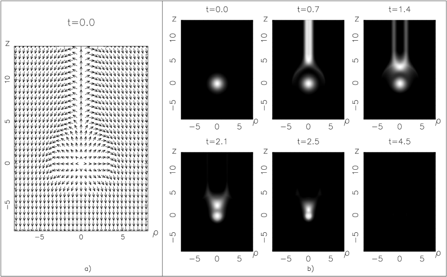
FIG. 1.: a) Plot of the scalar field $\Phi^{a}$ in the configuration given by eq. (12) in the text, for $r_{1}=3$, $r_{2}=6$, $a=0.9$, $b=1$. The configuration is axially symmetric. b) The result of numerical integration using a) as initial condition. Potential energy is shown in greyscale at different times. After annihilation of the monopole-antimonopole pair near $z=0$, the system fluctuates for some time until all the energy is radiated away (not shown; note the longer time elapsed between $t=2.5$ and $t=4.5$).

As explained in [6, 7], the shift (11) creates a tension pulling the monopole core, and the apparent unwinding (which starts in the inner shells) is only a manifestation of the core’s translation. In order to stop the motion of the core, we consider a hybrid configuration such that the monopole core remain unperturbed and the unwinding occur in the outer shells. This is achieved by taking $\xi=0$ for, say, $r<r_{1}$, a string-like configuration for $r>r_{2}$, and some continuous interpolation in between. One such configuration (see figure 1a) would be:

$${\hat{F}}(r,y)=f(r),\quad{\hat{\xi}}(r)=\left\{\begin{array}[]{ll}0&r<r_{1}\\ {\it c}\left(1-{{r_{1}}\over r}\right)&r_{1}<r<r_{2}\\ {\it a}+{\it b}\ln(r)&r_{2}<r\end{array}\right.$$ (12)

with ${\it a}\;\raise 1.29167pt\hbox{$>$\kern-7.5pt\raise-4.73611pt\hbox{$\sim$}}\;{\it a}_{0}$, ${\it b}\;\raise 1.29167pt\hbox{$>$\kern-7.5pt\raise-4.73611pt\hbox{$\sim$}}\;{\it b}_{0}$, and $c$ given by continuity of ${\hat{\xi}}(r)$.

If the energy (i.e. mass) inside $r_{2}$ is large enough there will be no appreciable motion of the monopole core (because the tension of the string is constant $\sim 4\pi$). For instance, simulations with $r_{1}=3$, $r_{2}=6$, ${\it b}=1$ show different behaviour depending on ${\it c}$: for ${\it c}\;\raise 1.29167pt\hbox{$<$\kern-7.5pt\raise-4.73611pt\hbox{$\sim$}}\;2.8$ the core translates, but for ${\it c}\;\raise 1.29167pt\hbox{$>$\kern-7.5pt\raise-4.73611pt\hbox{$\sim$}}\;2.8$, the unwinding happens far from the core, which remains fixed. In the latter case, the decay of the string can also be understood as a monopole-antimonopole pair creation with the new monopole appearing at $r=R$ and the antimonopole appearing near $r=r_{2}$. The equations solved in the simulations were

$$\Box\Phi^{a}+\Phi^{a}(|\Phi|^{2}-1)+\gamma\dot{\Phi}^{a}=0\quad,$$ (13)

with a dissipative term added to make the integration faster. Simulations using different $\gamma$ show no appreciable difference. The equations were integrated using cylindrical coordinates ($\rho,\varphi,z$) in a $200^{2}$ grid using explicit Runge-Kutta method with step size control [8]. The output can be seen in fig. 1b, where the potential energy is plotted at various times, confirming that the configuration (12) is unstable and decays to the vacuum.

We will now show that the extra energy required to reach this unstable configuration (12) from the spherical monopole configuration (2) is finite.

Consider the set of configurations with $F=f(r)$ and $\xi=\xi(r)$. From (10) the difference between the energy of any such configuration ($E[\xi]$) and the energy of the spherically symmetric unperturbed monopole ($E[0]$) is:

$$E[\xi]-E[0] = \left[\int_{0}^{r_{*}}+\int_{r_{*}}^{R}\right]\,{\rm{d}}r\,\left[{{r^{2}}\over 2}f^{2}(r)\xi_{r}^{2}(r)I[\xi(r)]\right]$$ (14)

$$I[\xi] = \int_{-\infty}^{+\infty}{\rm{d}}y\,{\rm sech}^{2}(y)\,{\rm sech}^{2}(y+\xi(r))\ \ .$$ (15)

$I[\xi]$ is bell-shaped: from a maximum value $I[0]=4/3$, it rapidly falls to zero for $|\xi|>\xi_{*}\approx 5$ as $\sim 16(|\xi|-1)exp({-2|\xi|})$. $r_{*}$ is the radius at which $\xi(r_{*})=\xi_{*}$. The first integral is clearly finite. The second can be estimated using the asymptotic form of $I[\xi]$ and is negligible for $\xi={\it a}+\ln r$ even in the limit $R\to\infty$, where one gets $\sim 16\,\pi e^{-{\it a}}\xi_{*}e^{-\xi_{*}}$.

Moreover, there is a continuous path in configuration space connecting the configurations (2) and (12) such that $E[\xi]-E[0]$ remains finite along the whole path: first increase $\xi$ in the outer shells $r>r_{*}$ using Goldhaber’s deformation ($\xi_{r}=0$) until $\xi$ reaches $\xi_{*}$; then adjust the radial dependence to match (12).

Thus, we have shown that the extra energy required by the monopole (2) to go over the energy barrier and decay to the vacuum is finite even as $R\to\infty$; moreover, since the monopole energy grows with R, the ratio $(E[{\hat{\xi}}]-E[0])/E[0]\to 0$ as $R\to\infty$.

IV Stability to small perturbations with axial symmetry

We now turn to the classical stability of (2) by considering small perturbations parametrised by

$$F=f(r)+\delta(t,r,y)$$ (16)

$$\tan({\bar{\theta}/2})=(1+\xi(t,r,y))e^{y} \qquad.$$ (17)

Neglecting quadratic terms gives $\sin\bar{\theta}\approx\sin\theta+\xi\sin\theta\cos\theta$,   $\cos\bar{\theta}\approx\cos\theta-\xi\sin^{2}\theta$. Introducing $X\equiv f\xi$,

$$\Phi^{1} \approx (f\sin\theta+\delta\sin\theta+X\sin\theta\cos\theta)\cos\varphi$$ (18)

$$\Phi^{2} \approx (f\sin\theta+\delta\sin\theta+X\sin\theta\cos\theta)\sin\varphi$$ (19)

$$\Phi^{3} \approx (f\cos\theta+\delta\cos\theta-X\sin^{2}\theta)\qquad,$$ (20)

which shows that the correct boundary conditions are that $\sin\theta(\delta+X\cos\theta)$ should vanish on the $z$ axis. Note that $\delta(0)$ and $X(0)$ need not vanish. An infinitesimal translation of the monopole in the $z$ direction corresponds to $\delta=-f_{r}(r)\cos\theta,\ X=f(r)/r$, and both $f_{r}(r)$ and $f(r)/r$ tend to $\approx 0.5$ as $r\to 0$ (see fig 2a ). There is no zero mode associated with global rotations since these have been factored out in the ansatz (7).

FIG. 2.: The functions: a) $f(r)/r$, $f_{r}(r)$; b)$V_{1}(r)$, $V_{2}(r)$.

As usual, the perturbation equations

$$0=r^{2}\Box\delta+2\delta+r^{2}[3f^{2}-1]\delta+2X_{y}-4X{\rm tanh}y$$ (21)

$$0={\rm sech}^{2}y\ r^{2}\Box X+{\rm sech}^{2}y[r^{2}(f^{2}-1)+2]X+2{\rm tanh}y\,X_{y}-2\delta_{y}$$ (22)

reduce to an eigenvalue problem in $\omega^{2}$ for perturbations of the form $\delta=e^{i\omega t}\hat{\delta}(r,y)$, $X=e^{i\omega t}\hat{X}(r,y)$. Eigenfunctions $\hat{\delta},\hat{X}$ with negative eigenvalues $\omega^{2}<0$ correspond to instabilities. Dropping hats and defining $u={\rm tanh}y$

$$R_{1}\delta+\partial_{u}[(u^{2}-1)\partial_{u}\delta]-2\partial_{u}[(u^{2}-1)X]=\omega^{2}r^{2}\delta$$ (23)

$$R_{2}X+\partial_{u}^{2}[(u^{2}-1)X]-2\partial_{u}\delta=\omega^{2}r^{2}X$$ , (24)

where $R_{1}$, $R_{2}$ are radial operators (see fig 2b):

$$R_{i}=-\partial_{r}(r^{2}\partial_{r})+V_{i}(r), \qquad i=1,2$$ (25)

$$V_{1}(r)=r^{2}(3f^{2}(r)-1)+2$$ (26)

$$V_{2}(r)=r^{2}(f^{2}(r)-1) \qquad.$$ (27)

Using Legendre polynomials and changing variables: $\chi:=\partial_{u}[(1-u^{2})X]=\sum\chi_{l}(r)P_{l}(u),\ \ \delta=\sum\delta_{l}(r)P_{l}(u)$ the equations for different values of $l$ decouple, giving

$$R_{1}\Delta_{l}+x^{2}\Delta_{l}+2x\chi_{l} =\omega^{2}r^{2}\Delta_{l}$$ (28)

$$R_{2}\chi_{l}+x^{2}\chi_{l}+2x\Delta_{l} =\omega^{2}r^{2}\chi_{l}$$ (29)

where we introduced $x=\sqrt{l(l+1)}$ and $\Delta_{l}=x\delta_{l}$. In order to get (29) we multiplied the $X$ eqn. in (24) by $(1-u^{2})$ and differentiated w.r.t. $u$, so there may be spureous solutions; in particular, $l=0$ corresponds to angular perturbations that are singular on the $z$ axis. These are not physical, and will be discarded. But if there is no solution of (28,29) with negative $\omega^{2}$ there will be no instability in the original problem (22).

Our task is to find the solution to (28,29) with the minimum value of $\omega^{2}$ over all admissible perturbations and all $l\geq 1$. We know one $l=1$ solution, the translational zero mode ($\tilde{\Delta}_{1}=\sqrt{2}f_{r}(r)$, $\tilde{\chi}_{1}=-2\,f(r)/r$). Goldhaber’s deformation ($\chi_{1}=f(r)$, $\Delta_{1}=0$) is also $l=1$ but is not a solution of (28, 29), and it can be shown that there are no instabilities with $\chi_{1}(r\to\infty)\sim\rm{const}$.

Let us first consider normalizable perturbations. Note that, for each $l$, the equations (28,29) can be obtained by functional variation from

$$E_{l}\equiv\int{\rm{d}}r\left[r^{2}\left(\Delta_{r}^{2}+\chi_{r}^{2}\right)+(V_{1}+x^{2})\Delta^{2}+(V_{2}+x^{2})\chi^{2}+4x\Delta\chi\right]=\omega^{2}\int{\rm{d}}rr^{2}[\Delta^{2}+\chi^{2}]\qquad.$$ (30)

The lowest value of $\omega^{2}$ can be found minimising $E_{l}$ over normalized functions, $\int{\rm{d}}rr^{2}[\Delta^{2}+\chi^{2}]=1$ and over all $l\geq 1$. However the minimum must be in the $l=1$ sector since, for all $l>1$ and for given $\Delta$,$\chi$, $(E_{l}-E_{1})$ is a sum of squares with positive coefficients:

$$E_{l}-E_{1}=\int{\rm{d}}r[A_{l,+}(\Delta+\chi)^{2}+A_{l,-}(\Delta-\chi)^{2}]\ ,$$ (31)

where $A_{l,\pm}\equiv[x^{2}-2\pm 2(x-\sqrt{2})]/2\ >\ 0$ for $l>1$.

In order to investigate the $l=1$ sector, we rewrite $E_{1}$ using arbitrary functions $G(r)$, $H(r)$ and $K(r)$:

$$E_{1}=\int_{0}^{\infty}{\rm{d}}r\left[\left(r\Delta_{r}+\frac{G}{r}\Delta\right)^{2}+\left(r\chi_{r}+\frac{H}{r}\chi\right)^{2}+2\sqrt{2}\,\left(\frac{\Delta}{K}+K\chi\right)^{2}+\left(V_{1}+2-\frac{2\sqrt{2}}{K^{2}}+G_{r}-\frac{G^{2}}{r^{2}}\right)\chi^{2}\right.$$ (32)

$$\left.+\left(V_{2}+2-2\sqrt{2}K^{2}+H_{r}-\frac{H^{2}}{r^{2}}\right)\Delta^{2}\right]-\left.G(r)\Delta^{2}(r)\right|_{0}^{\infty}+\left.H(r)\chi^{2}(r)\right|_{0}^{\infty} \qquad.$$ (33)

Choosing $G(r)=-r^{2}\partial_{r}\ln\tilde{\Delta}_{1}$, $H(r)=-r^{2}\partial_{r}\ln\tilde{\chi}_{1}$, $K(r)^{2}=-{\tilde{\Delta}_{1}}/{\tilde{\chi}_{1}}$, the coefficients of $\Delta^{2}$ and $\chi^{2}$ in (33) vanish identically by virtue of (3). For large r, $G$ and $H\sim r$, thus, $E_{1}\geq 0$ for all functions ($\Delta_{1}$, $\chi_{1}$) that decay faster than $1/\sqrt{r}$ as $r\to\infty$. This proves that all normalizable perturbations have $\omega^{2}\geq 0$. The above argument and a host of numerical simulations strongly suggest that non-normalizable perturbations are at best compatible with $\omega^{2}=0$, as can be verified directly from the equations for perturbations that fall to zero like a power of r, but in this case we have no analytic proof.

V Discussion

In this paper we have derived and analysed the axial perturbation equations of $O(3)$ monopoles and proved that, contrary to statements in the literature, $O(3)$ monopoles are perturbatively stable (or neutrally stable) to infinitesimal, axially symmetric, normalizable (or power-law decay) perturbations. We have also proved that the energy barrier between topological sectors is finite, irrespective of the details of the scalar potential. This feature is specific of global monopoles; global vortices in two dimensions, whose energy grows logarithmically with radius, and gauge monopoles, whose energy is finite, are separated from the vacuum by an energy barrier growing linearly with the cut-off. But the energy of global monopoles is dominated by two-dimensional (angular) gradients far from the core, and these can be deformed with no energy cost.

One would naively expect thermal fluctuations with $KT\sim E[\xi]-E[0]$ to cause the monopole to decay. As far as we know, this effect is not seen in “cosmological” numerical simulations of global monopole networks, but perhaps this is not so surprising. First, we worked in flat space. Second, the range of scales introduced by the expansion of the Universe forces drastic approximations on cosmological simulations; in particular, the sigma model approximation, which is widely used, sets the field on the vacuum manifold everywhere, so unwinding and pair creation events are not resolved by the grid. Finally, cosmological simulations do not include thermal effects, and it has been shown that full thermal simulation across the phase transition [10] gives qualitatively different results. Our results provide further evidence that a more careful analysis of global monopole networks may be required.

 

VI Acknowledgments

We thank M. J. Esteban for pointing out an error in an earlier version of this paper, and M. Escobedo, R. Durrer, R. Gregory, A. Vilenkin, K. Kuijken, I.L. Egusquiza, J.M. Aguirregabiria, L. Perivolaropoulos and A. Lande for conversations. We acknowledge support from grants CICYT AEN99-0315 and UPV 063.310-EB225/95.

REFERENCES

- [1] A. Vilenkin, E. P. S. Shellard, Cosmic Strings and Other Topological Defects, Cambridge University Press, Cambridge (1994), and references therein.
- [2] See, e.g. J. Magueijo, R.H. Brandenberger, preprint, astro-ph/0002030, and references therein.
- [3] R. Durrer, M. Kunz, A. Melchiorri, preprint, astro-ph/9901377; R. Durrer, in ”Energy Densities in the Universe”, proceedings of the XXXVth Rencontres de Moriond, edited by Jacques Dumarchez, to be published (astro-ph/0003363).
- [4] M. Barriola, A. Vilenkin, Phys. Rev. Lett. 63 (1989) 341.
- [5] A. S. Goldhaber, Phys. Rev. Lett. 63 (1989) 2158.
- [6] S. H. Rhie, D. P. Bennett, Phys. Rev. Lett. 67 (1991) 1173.
- [7] L. Perivolaropoulos Nucl. Phys. B375 (1992) 665.
- [8] The code “dopri5”, by Dormand&Prince, is described in E. Hairer, S.P. Norsett and G. Wanner, Solving ordinary differential equations I, nonstiff problems, Springer Series in Computational Mathematics, Springer-Verlag (1993).
- [9] Inequalities, edition (p. 244) G. Hardy, J.E. Littlewood & G.Pólya, Cambridge University Press 1973.
- [10] N. D. Antunes, L. M. A. Bettencourt, A. Yates, preprint, hep-ph/9901391.