MZ-TH/99-11

Analyticity, crossing and the absorptive parts of the one-loop contributions to the quark-quark-gluon gauge boson four-point function

ABSTRACT

Starting from the known one-loop result for the $e^{+}e^{-}$-annihilation process $e^{+}e^{-}\stackrel{{\scriptstyle\gamma,Z}}{{\longrightarrow}}q\bar{q}g$ with massless quarks we employ analyticity and crossing to determine the absorptive parts of the corresponding one-loop contributions in Deep Inelastic Scattering (DIS) and in the Drell-Yan process (DY). Whereas the ${\cal O}(\alpha_{s}^{2})$ absorptive parts generate a non-measurable phase factor in the $e^{+}e^{-}$-annihilation channel one obtains measurable phase effects from the one-loop contributions in the deep inelastic and in the Drell-Yan case. We compare our results with the results of previous calculations where the absorptive parts in DIS and in the DY process were calculated directly in the respective channels. We also present some new results on the dispersive and absorptive contributions of the triangle anomaly graph to the DIS process.

I Introduction

Some time ago, after QCD started to become established as the theory of hadronic interactions, a number of authors looked into the possibility of measuring $T$-odd effects in current-induced interaction that would result from QCD rescattering effects. The rescattering effects were calculated from the absorptive parts of the relevant next-to-leading order QCD one-loop contributions.

The authors of [1] considered $T$-odd effects in the decay of a $J^{PC}=1^{--}$ quarkonium state into three gluonic jets. $T$-odd effects in $e^{+}e^{-}$-annihilation into three partonic jets were considered in [2, 3, 4] excepting quark loop contributions. First, it came as a surprise that, for mass zero quarks, there are no leading order ${\cal O}(\alpha_{s}^{2})$ $T$-odd effects in this reaction [2]. This was understood more systematically later on in [5, 6] from the observation that the absorptive parts are necessarily proportional to the Born term and are thus unobservable. Measurable $T$-odd effects in these reactions are generated by quark mass effects which were investigated in [3, 4]. The non-observability of ${\cal O}(\alpha_{s}^{2})$ $T$-odd effects in $e^{+}e^{-}$-interactions for the massless case does not carry over to the crossed channels of deep inelastic scattering (DIS) and the Drell-Yan (DY) process. $T$-odd effects in DIS were explored in [5, 7] and in the DY process in [8].

Since the early proposals to measure $T$-odd effects in current induced interactions in the early eighties experimental facilities and techniques have considerably been improved. Luminosities of lepton-hadron and hadron-hadron colliders have dramatically increased providing for much higher event rates than was possible in the earlier experiments. The energy range of the collliders has been extended such that high momentum transfers can now be routinely probed. For example, at HERA one is starting to probe weak interaction $Z$-exchange effects in neutral current events at very high momentum transfers. This opens the door for the investigation of $T$- and $P$-odd effects in neutral current DIS. Powerful jet finding and flavour tagging algorithms have been developed that allow one to define asymmetry measures related to $T$-odd effects in DIS that use parton jet observables instead of the semi-inclusive particle observables used in the calculation of [5, 7, 9]. Finally, there have been dramatic improvements in the availability of polarized beams which again can be utilized to define new $T$-odd observables [10].

It is therefore timely to take a fresh look at the subject of $T$-odd observables in current- induced reactions generated by QCD rescattering effects or, in a different language, by the absorptive parts of the corresponding one-loop contributions. In this paper we point out that the ${\cal O}(\alpha_{s}^{2})$ absorptive parts of the relevant one-loop contributions in DIS and in the DY process can be obtained through crossing from the well-known one-loop contributions to $e^{+}e^{-}\rightarrow q\overline{q}g$ annihilation calculated in [6]. This is theoretically appealing and provides an independent check of the results presented before in DIS [5, 7] and DY [8]. We also fill out some small odds and ends on the subject of $T$-odd observables in these reactions which had not been covered in the earlier publications.

Our paper is structured as follows. In Sec. 2 we derive crossing rules that allow one to cross from the $e^{+}e^{-}$-annihilation channel to the DIS and DY channels. To obtain the absorptive parts in the respective channels it is necessary to discuss the analyticity structure of the one-loop contributions in the complex plane of the relevant kinematical variables. The absorptive parts originate from logarithmic and dilogarithmic functions in the one-loop amplitude when their arguments take values on cuts in the analytic plane. We identify the range of values of the kinematical variables in the three processes and show how to analytically continue the one-loop functions from the $e^{+}e^{-}$-channel to the DIS and DY channels. Sec. 3 is devoted to a detailed discussion of $T$-odd effects in DIS. We first provide a complete list of the nonsingular one-loop contributions in $e^{+}e^{-}$-annihilation. Using the crossing rules laid down in Sec. 2 we analytically continue the one-loop amplitudes to DIS. The absorptive one-loop amplitudes are then folded with the Born term contributions. There are three $T$-odd hadronic structure functions, $H_{5}$, $H_{8}$, and $H_{9}$, whose functional form is given for the quark, antiquark and gluon initiated cases. We then define helicity structure functions which appear as angular coefficients in the angular decay distribution of the DIS process when the hadronic tensor is folded with the leptonic tensor. This allows us to compare our results with the results of [5, 7]. We find complete agreement with the $T$-odd results presented in these papers. In Sec. 4 we do the crossing and the analytical continuation to the DY process. Again we find agreement of our results for the $T$-odd structures with those given in [8] after corrections for a typographical error reported in [11]. In Sec. 5 we give our summary and provide an outlook on possible further applications of our results to spin-dependent $T$-odd observables. In an Appendix we present results on the dispersive and absorptive contributions of the triangle anomaly graph to the DIS process.

II General principles of analyticity and crossing

In this chapter we will develop the framework necessary to obtain the ${\cal O}(\alpha_{s}^{2})$ one-loop corrections in the DIS and DY channels from the known results in the $e^{+}e^{-}$-annihilation channel [6]. In particular, we will derive crossing rules that allow one to determine the whole set of invariant hadronic structure functions $H_{i}$ (i=1,…,9), including the absorptive $T$-odd structure functions for the DIS and the DY processes.

In the absence of polarisation the definition of $T$-odd observables in current-induced interactions involves the analysis of parton processes with at least three partons necessary to form triple momentum products. In order to fix our notation let us write down the momentum configuration for $e^{+}e^{-}$ annihilation into a quark, antiquark and a gluon:

$$l^{-}(k)+l^{+}(k^{\prime})\stackrel{{\scriptstyle\gamma,Z}}{{\longrightarrow}}q(p_{1})+\bar{q}(p_{2})+g(p_{3})$$ (1)

where $l^{-}$ and $l^{+}$ are massless leptons, $q$ and $\bar{q}$ are massless quarks and antiquarks, respectively, and $g$ is a bremsstrahlung gluon. The momentum of the time-like gauge boson is determined from four-momentum conservation and is given by $q=p_{1}+p_{2}+p_{3}$.

The leading order contributions to the $T$-odd observables come from the interference of the absorptive parts of the one-loop amplitudes and the Born term amplitude. In Fig. 1 we show the ${\cal O}(\alpha_{s}^{2})$ one-loop diagrams that contribute to $e^{+}e^{-}\rightarrow q\bar{q}g$ (with the leptonic part omitted). They divide into the eleven contributions without quark loops and the two diagrams with a quark loop. In the main part of this paper we will be mostly concerned with the first eleven non-quark loop contributions (a) - (k). A discussion of the so-called triangle-anomaly quark loop contributions (l) and (m) is deferred to the Appendix.

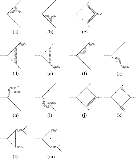
FIG. 1.: ${\cal O}(\alpha_{s}^{2})$ one-loop corrections to the $e^{+}e^{-}$ annihilation.

At the three-parton level DIS proceeds through the following three subprocesses:

$$l(k)+q(p) \stackrel{{\scriptstyle\gamma,Z,W^{\pm}}}{{\longrightarrow}} l^{\prime}(k^{\prime})+q(p^{\prime})+g(p_{3}),$$ (2)

$$l(k)+\bar{q}(p) \stackrel{{\scriptstyle\gamma,Z,W^{\pm}}}{{\longrightarrow}} l^{\prime}(k^{\prime})+\bar{q}(p^{\prime})+g(p_{3}),$$ (3)

$$l(k)+g(p) \stackrel{{\scriptstyle\gamma,Z,W^{\pm}}}{{\longrightarrow}} l^{\prime}(k^{\prime})+q(p^{\prime})+\bar{q}(p_{3}).$$ (4)

They are referred to as the quark-, antiquark- and gluon-initiated DIS processes, respectively. The momentum of the space-like gauge boson is now given by $q=-p+p^{\prime}+p_{3}$.

In the DY process the next-to-leading order contributions come from the following subprocesses:

$$q(p_{a})+\overline{q}(p_{b}) \stackrel{{\scriptstyle\gamma,Z,W^{\pm}}}{{\longrightarrow}} l(k)+l^{\prime}(k^{\prime})+g(p_{3}),$$ (5)

$$q(p_{a})+g(p_{b}) \stackrel{{\scriptstyle\gamma,Z,W^{\pm}}}{{\longrightarrow}} l(k)+l^{\prime}(k^{\prime})+q(p_{3}),$$ (6)

$$\overline{q}(p_{a})+g(p_{b}) \stackrel{{\scriptstyle\gamma,Z,W^{\pm}}}{{\longrightarrow}} l(k)+l^{\prime}(k^{\prime})+\overline{q}(p_{3}),$$ (7)

where (5) is the annihilation subprocess and (6) and (7) are the so-called quark- and antiquark-initiated ”Compton” subprocesses, respectively. The momentum of the time-like gauge boson is given by $q=p_{a}+p_{b}-p_{3}$. Differing from $e^{+}e^{-}$-annihilation there are also charged gauge boson contributions to DIS and the DY process.

In what follows we need to discuss only the hadronic part of the three-parton processes listed in (2) and (5-7). The contraction with the leptonic part will lead to angular factors and some $y$-dependence in the DIS case. The contraction with the leptonic tensor will be discussed in the subsequent sections when we compare our results with the calculation of Hagiwara et al. [5, 7, 8].

The relevant one-loop contributions to DIS and the DY process can be obtained from the one-loop contibutions to $e^{+}e^{-}$-annihilation calculated in [6] through crossing, i.e. through the exchange of incoming and outgoing particle momenta in the one-loop diagrams in Fig.1. For the real parts of the one-loop contributions and for the Born term contribution crossing can be implemented in a straightforward manner. Crossing is more subtle for the imaginary parts of the one-loop amplitudes and needs a careful discussion of the analyticity properties of the one-loop amplitude.

The crossing of external lines in Feynman diagrams implies a sign change of the four momentum associated with that line. Thereby, the values of the kinematic variables associated with the respective momentum undergoes a discontinuous change. Massless one-loop amplitudes contain log and dilog functions which depend on these kinematic variables and which may be indefinite in certain ranges of their domains of definition, i.e. they may be multivalued. One can choose among the possible values by defining the value of the function at a given point. Starting from this point one determines the value of the multivalued function on the cuts by analytic continuation. The kinematic variables are taken to be complex in this procedure.

In order to obtain a smooth continuation one makes use of the imaginary parts of the one-loop amplitudes given by the ($i\tau$)-form of the relevant propagators. In this way one avoids possible ambiguities. As an example we take the natural logarithm. The logarithm is taken as a complex-valued analytic function with a cut on the negative real axis and a branch point located at zero.

Next consider the natural logarithm of an arbitrary positive real number $x$. To obtain its value at ($-x$) we use

$\displaystyle\ln(-x)=\ln(|x|)+i(2k+1)\pi,{\rm\hskip 14.45377pt}{\rm with}{\rm\hskip 14.45377pt}k\in{\cal Z}.$

The integer number $k$ will be determined from the phase angle of the complex number ($-x$). If one excludes multiple rotations in the complex plane then one remains with only two possibilities: $k=0,-1$. For all complex numbers of the form ($-x\pm i\tau$) with an infinitesimally small positive $\tau$ one would have the following identity:

$$\lim_{\tau\rightarrow 0}\ln(-x\pm i\tau)=\ln(|x|)\pm i\pi.$$ (8)

The results of the calculation of the one-loop contributions to $e^{+}e^{-}$-annihilation listed in [6] contain no explicit $i\tau$ prescription. This is adequate for the $e^{+}e^{-}$-reaction since in this case the results are given for regions in the complex plane away from the singularities. The results are valid only in this restricted region and need to be analytically continued to the other regions in the complex plane accessible in DIS and in the DY case. It is, however, possible to restore the omitted $i\tau$ prescriptions in [6] in a straightforward way. For the relevant kinematic variables the infinitesimal imaginary parts are provided by the Feynman rules if one takes the full propagators in their original ($i\tau$)-form. In this case one has the following terms from solving the loop integrals $(s_{ij}\equiv(p_{i}+p_{j})^{2}=2p_{i}p_{j})$:

$$\frac{s_{ij}+i\tau}{q^{2}+i\tau},{\rm\hskip 14.45377pt}1-\frac{s_{ij}+i\tau}{q^{2}+i\tau},{\rm\hskip 14.45377pt}{\rm and}{\rm\hskip 14.45377pt}(-q^{2}-i\tau)^{-\varepsilon},$$ (9)

where ${\varepsilon}=2-d/2$, and $d$ is the continuous space-time dimension.

Here one should notice that the form of energy-momentum conservation for the s-channel annihilation ensures relative plus signs between the three scalar invariants $s_{ij}=2p_{i}p_{j}$ and $i\tau$, as well as between $q^{2}$ and $i\tau$ in the denominators of the respective Feynman integrals. Thus, more generally, one has the following rules for s-channel annihilation:

$$q^{2}\rightarrow q^{2}+i\tau,{\rm\hskip 28.90755pt}s_{ij}\rightarrow s_{ij}+i\tau.$$ (10)

With these rules the results of [6] are valid in any kinematical region.

For the kinematical variables $y_{ij}=s_{ij}/q^{2}$ used in [6] one finds the following replacements:

$$y_{ij} \rightarrow y_{ij}+\frac{i\tau}{q^{2}}(1-y_{ij})+{\cal O}(\tau^{2}),$$ (11)

$$1-y_{ij} \rightarrow 1-y_{ij}-\frac{i\tau}{q^{2}}(1-y_{ij})+{\cal O}(\tau^{2}),$$ (12)

$$(-q^{2})^{-\varepsilon} \rightarrow 1-\varepsilon\ln(-q^{2}-i\tau)+{\cal O}(\varepsilon^{2}).$$ (13)

For every contributing subprocess in DIS and DY one has to perform a detailed investigation of the range of values of the $y_{ij}$’s after crossing and then one can analytically continue the log and dilog functions and thereby remove the ambiguity which occurs when one changes the sign of their arguments. The analytic continuation of the logarithm function is given in (8). For the dilogarithms, when $x>1$, we use the identity

$${\rm Li}_{2}(x)=-{\rm Li}_{2}(1-x)+\zeta(2)-\ln(x)\ln(1-x),$$ (14)

and treat the complex logarithm $\ln(1-x)$ according to (8).

At this point we introduce the usual hadronic DIS variables $x$ and $z$

$$x=\frac{-q^{2}}{2qp},{\rm\hskip 32.52127pt}z=\frac{pp^{\prime}}{qp}\,,$$ (15)

and proceed with the crossing procedure as described above. The crossing from the $e^{+}e^{-}$-channel to the quark-initiated subprocesses in DIS is given by the following change of the momenta

$$p_{1}\rightarrow p^{\prime}\qquad{\rm and}\qquad p_{2}\rightarrow-p\,,$$ (16)

according to the momentum definitions in (1) and (2). The change of the kinematical variables $y_{ij}$’s and the new ranges of their values are given by

$$y_{12}\equiv\frac{2p_{1}p_{2}}{q^{2}}\rightarrow y_{12}^{q}\equiv\frac{2pp^{\prime}}{-q^{2}} = \frac{z}{x}{\rm\hskip 32.52127pt}\in[1,\infty]\,,$$ (17)

$$y_{13}\equiv\frac{2p_{1}p_{3}}{q^{2}}\rightarrow y_{13}^{q}\equiv\frac{2p^{\prime}p_{3}}{q^{2}} = 1-\frac{1}{x}{\rm\hskip 14.45377pt}\in[-\infty,0]\,,$$ (18)

$$y_{23}\equiv\frac{2p_{2}p_{3}}{q^{2}}\rightarrow y_{23}^{q}\equiv\frac{2pp_{3}}{-q^{2}} = \frac{1-z}{x}{\rm\hskip 14.45377pt}\in[1,\infty]\,.$$ (19)

One should note that $q^{2}<0$ in the crossed DIS channel. The corresponding crossing to the antiquark-initiated subprocess involves the momentum changes $p_{1}\rightarrow-p$ and $p_{2}\rightarrow p^{\prime}$. However, we need not explicitly discuss crossing for this case since one can use $CP$-invariance in the final result for the quark-initiated case to obtain the corresponding antiquark-initiated results.

Similarly, the crossing from the $e^{+}e^{-}$-annihilation to the gluon-initiated subprocess in DIS is effected by

$$p_{1}\rightarrow p^{\prime}\qquad{\rm and}\qquad p_{3}\rightarrow-p\,.$$ (20)

The resulting $y_{ij}^{g}$’s are:

$$y_{12}\rightarrow y_{12}^{g}\equiv\frac{2p^{\prime}p_{2}}{q^{2}} = 1-\frac{1}{x}{\rm\hskip 14.45377pt}\in[-\infty,0],$$ (21)

$$y_{13}\rightarrow y_{13}^{g}\equiv\frac{2pp^{\prime}}{-q^{2}} = \frac{z}{x}{\rm\hskip 32.52127pt}\in[1,\infty],$$ (22)

$$y_{23}\rightarrow y_{23}^{g}\equiv\frac{2pp_{2}}{-q^{2}} = \frac{1-z}{x}{\rm\hskip 14.45377pt}\in[1,\infty].$$ (23)

The one-loop results in [6] are presented in terms of the variables $x_{k}=2p_{k}q/q^{2}$ $(k=1,2,3)$. The $x_{k}$ are related to the $y_{ij}$ via

$\displaystyle x_{k}=1-y_{ij},{\rm\hskip 28.90755pt}(k\not=i,j).$

Next we turn to the Drell-Yan process. For the annihilation subprocess (5) crossing implies the following change of momenta

$$p_{1}\rightarrow-p_{a}\qquad{\rm and}\qquad p_{2}\rightarrow-p_{b}\,.$$ (24)

For the quark-initiated ”Compton” scattering one has to change

$$p_{1}\rightarrow-p_{a}\qquad{\rm and}\qquad p_{3}\rightarrow-p_{b}\,,$$ (25)

with $q\rightarrow-q$ in both cases. Again we omit explicit reference to the antiquark-initiated ”Compton” scattering case because its structure follows from the quark-initiated ”Compton” scattering case through $CP$ invariance.

The corresponding kinematical variables in the annihilation subprocesses are now

$$y_{12}\rightarrow y_{12}^{a}\equiv\frac{2p_{a}p_{b}}{q^{2}} = \frac{1}{x_{a}}+\frac{1}{x_{b}}-1{\rm\hskip 14.45377pt}\in[1,\infty]\,,$$ (26)

$$y_{13}\rightarrow y_{13}^{a}\equiv-\frac{2p_{a}p_{3}}{q^{2}} = 1-\frac{1}{x_{b}}{\rm\hskip 36.135pt}\in[-\infty,0]\,,$$ (27)

$$y_{23}\rightarrow y_{23}^{a}\equiv-\frac{2p_{b}p_{3}}{q^{2}} = 1-\frac{1}{x_{a}}{\rm\hskip 36.135pt}\in[-\infty,0]\,.$$ (28)

The crossed $y_{ij}$’s for the quark-initiated ”Compton” subprocesses are

$$y_{12}\rightarrow y_{12}^{C_{q}}\equiv-\frac{2p_{a}p_{3}}{q^{2}} = 1-\frac{1}{x_{b}}{\rm\hskip 43.36243pt}\in[-\infty,0]\,,$$ (29)

$$y_{13}\rightarrow y_{13}^{C_{q}}\equiv\frac{2p_{a}p_{b}}{q^{2}} = \frac{1}{x_{a}}+\frac{1}{x_{b}}-1{\rm\hskip 25.29494pt}\in[1,\infty]\,,$$ (30)

$$y_{23}\rightarrow y_{23}^{C_{q}}\equiv-\frac{2p_{b}p_{3}}{q^{2}} = 1-\frac{1}{x_{a}}{\rm\hskip 43.36243pt}\in[-\infty,0]\,.$$ (31)

TABLE I.: Imaginary parts of different functions appearing after crossing from $e^{+}e^{-}$-annihilation to the quark- and gluon-initiated cases in DIS, denoted by $\rm DIS^{q}$ and $\rm DIS^{g}$, respectively, and to the annihilation ($\rm DY^{a}$) and ”Compton” ($\rm DY^{C}$) subprocesses in DY. The invariants $y_{ij}^{q}$, $y_{ij}^{g}$, $y_{ij}^{a}$ and $y_{ij}^{C}$ are defined in (17), (21), (26) and (29)

functions	$\rm DIS^{q}$	$\rm DIS^{g}$		$\rm DY^{a}$	$\rm DY^{C}$
$\ln(y_{12})$	0	$-i\pi$		0	$i\pi$
$\ln(1-y_{12})$	$-i\pi$	0		$i\pi$	0
${\rm Li}_{2}(y_{12})$	$i\pi\ln(y_{12}^{q})$	0		$-i\pi\ln(y_{12}^{a})$	0
$\ln(y_{13})$	$-i\pi$	0		$i\pi$	0
$\ln(1-y_{13})$	0	$-i\pi$		0	$i\pi$
${\rm Li}_{2}(y_{13})$	0	$i\pi\ln(y_{13}^{g})$		0	$-i\pi\ln(y_{13}^{C})$
$\ln(y_{23})$	0	0		$i\pi$	$i\pi$
$\ln(1-y_{23})$	$-i\pi$	$-i\pi$		0	0
${\rm Li}_{2}(y_{23})$	$i\pi\ln(y_{23}^{q})$	$i\pi\ln(y_{23}^{g})$		0	0

In the above equation we have introduced the DY variables $x_{a}$ and $x_{b}$ defined by

$$x_{a}=\frac{M^{2}}{2qp_{a}},{\rm\hskip 32.52127pt}x_{b}=\frac{M^{2}}{2qp_{b}}\,,$$ (32)

where $M^{2}$ is the mass of the exchanged gauge bosons $W^{\pm}$ and $Z$, or, for the electromagnetic interaction, one has $M^{2}=q^{2}$.

Note the $2\leftrightarrow 3$ symmetry between the annihilation and the quark-initiated Compton subprocess in terms of the subprocess variables $x_{a}$ and $x_{b}$. The momentum changes involved in crossing from the $e^{+}e^{-}$-channel to DIS and the DY channel are summarized in Fig. 2 using diagram 1(f) as an illustrative example.

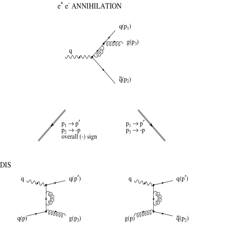
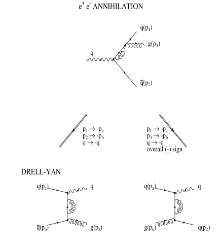
FIG. 2.: Illustration of crossing from $e^{+}e^{-}$-annihilation to the DIS and DY processes for one representative one-loop contribution. Shown are crossing to the quark- and gluon-initiated DIS processes and the annihilation and quark-initiated Compton processes in DY.

As we have already mentioned before, the results of the calculation in $e^{+}e^{-}$-annihilation channel contain log and dilog functions, which, after applying the rules from (17-21) and from (26-29) have to be analytically continued to the new kinematically allowed regions. Using the cut structure defined in (8) and (14), one obtains their absorptive parts. The results of crossing and analytic continuation of logarithmic and dilogarithmic functions appearing in our calculation of $T$-odd amplitudes in DIS and DY channels are summarized in Table I.

III Crossing Results for Hadronic Structure Functions in DIS

We now proceed to derive the $T$-odd hadronic structure functions in DIS by applying the analyticity and crossing rules derived in the proceeding section starting with the $e^{+}e^{-}$ results in [6]. We will be mostly interested in the imaginary (absorptive) parts but will also briefly comment on the crossing properties of the real parts of the one-loop amplitudes and the Born term amplitudes. The results of the crossing procedure will then be compared to the corresponding results in DIS in the three quark, antiquark and gluon-initiated cases [5, 7]. As was mentioned in the introduction, the $T$-odd structure functions in the $e^{+}e^{-}$ case vanish identically at the one-loop level for the set of graphs (1a)-(1k) with no quark loops. The reason is that the absorptive parts of the $e^{+}e^{-}$-annihilation massless one-loop amplitudes are proportional to the singular terms of its dispersive part which in turn have Born term structure [2, 6]. The absorptive parts are thus not measurable at this order of perturbation theory. However, the kinematics is different in the crossed processes and this proportionality no longer holds leading to nonvanishing $T$-odd effects in the crossed channels.

We begin our discussion by recapitulating the $e^{+}e^{-}$-annihilation one-loop results given in [6]. They are needed as a starting point for the crossing procedure. The transition amplitude $T^{V}_{\mu\beta}$ for the vector current transition $V_{\mu}\rightarrow q\bar{q}g$ can be expanded in $d$-dimensions along the seven independent covariants [6]

$$T^{V}_{\mu\beta} = N_{i}\;C^{i}_{\mu\beta}\qquad\qquad\qquad(i=1,...,7)$$ (33)

$$= q^{-4}N_{1}\;\hat{p}_{+\mu}\tilde{p}_{-\beta}\not p_{3}+q^{-4}N_{2}\;\hat{p}_{-\mu}\tilde{p}_{-\beta}\not p_{3}$$ (37)

$$+q^{-2}N_{3}\;\hat{\gamma}_{\mu}\tilde{p}_{-\beta}+q^{-2}N_{4}\;\hat{p}_{+\mu}\tilde{\gamma}_{\beta}$$

$$+q^{-2}N_{5}\;\hat{p}_{-\mu}\tilde{\gamma}_{\beta}+q^{-2}N_{6}\;\hat{\tilde{g}}_{\mu\beta}\not p_{3}$$

$$+N_{7}\left(\gamma_{\mu}\frac{\not p_{2}+\not p_{3}}{s_{23}}\gamma_{\beta}-\gamma_{\beta}\frac{\not p_{1}+\not p_{3}}{s_{13}}\gamma_{\mu}\right)$$

where $q=p_{1}+p_{2}+p_{3}$ and $p_{\pm}=p_{1}\pm p_{2}$. The covariants $C^{i}_{\mu\beta}$ are defined through Eq. (33) and the symbols “$\sim$” and “$\wedge$” denote the gauge invariant completions

$$\hat{p}_{\mu} = p_{\mu}-\frac{pq}{q^{2}}q_{\mu}\,,$$ (38)

$$\hat{\gamma}_{\mu} = \gamma_{\mu}-\frac{\not q}{q^{2}}q_{\mu}\,,$$ (39)

$$\tilde{p}_{\beta} = p_{\beta}-\frac{pp_{3}}{p_{3}q}q_{\beta}\,,$$ (40)

$$\tilde{\gamma}_{\beta} = \gamma_{\beta}-\frac{\not p_{3}}{p_{3}q}q_{\beta}\,,$$ (41)

$$\hat{\tilde{g}}_{\mu\beta} = g_{\mu\beta}-\frac{q_{\beta}p_{3\mu}}{p_{3}q}\,.$$ (42)

In writing down the covariant expansion it is understood that the covariants are taken between the relevant spin wave functions, i.e. $\bar{u}_{1}T^{V}_{\mu\beta}v_{2}\varepsilon^{*\beta}$.

We emphasize that the $T$-odd structure functions resulting from the one-loop amplitudes are infrared (IR) and collinear (M) finite in $d=4$ dimensions. This follows indirectly from the Lee-Nauenberg theorem in that there are no corresponding tree graph contributions that could cancel the divergencies if there were any. We could in principle therefore keep $d=4$ in our calculation. In this case one has overcounted the number of covariants in the above expansion. There are in fact only six independent covariants in four dimensions as can be verified by counting the number of independent helicity amplitudes. For the sake of completeness we list the linear relation between the seven covariants $C^{i}_{\mu\beta}$ in $d=4$ dimensions (taken between spin wave functions) which can be obtained from [13, 14]. One has

$$(1-x_{1})(1-x_{2})(1-x_{3})C^{7}_{\mu\beta} = x_{3}C^{1}_{\mu\beta}-\frac{1}{2}x_{3}(x_{1}+x_{2})C^{3}_{\mu\beta}-\frac{1}{2}(x_{1}^{2}-x_{2}^{2})C^{4}_{\mu\beta}$$ (44)

$$+\frac{1}{2}x_{3}^{2}C^{5}_{\mu\beta}-(x_{1}-x_{2})(1-x_{3})C^{6}_{\mu\beta}.$$

As concerns the present application it is nevertheless technically advantageous to work with the (overcounted) set of the above seven covariants. Note that the seventh covariant $C^{7}_{\mu\beta}$ in (33) has been chosen to have Born term structure. This will be important to keep in mind in what follows. As we are dealing with massless quarks the case of axial vector current transition $A_{\mu}\rightarrow q\bar{q}g$ can be easily dealt with. We simply have to multiply the vector current amplitude by $\gamma_{5}$ from the left. One has

$$T^{A}_{\mu\beta}=\gamma_{5}T^{V}_{\mu\beta}\,.$$ (45)

What is needed are explicit forms of the one-loop amplitudes in the $e^{+}e^{-}$ channel. The IR and M singular one-loop contributions have Born term structure and will not be needed in the following. As concerns the nonsingular one-loop contributions, we decided to reproduce the two relevant tables, Table II and Table III, from [6] because the results of [6] may not be readily available to everyone (in those early days there was no electronic publishing).

There are two colour structures in the one-loop amplitudes referred to as the QCD and QED structure. The corresponding amplitudes are denoted by $\tilde{N}_{i}$ (Table II) and $\hat{N}_{i}$ (Table III), respectively,

$\displaystyle N_{l}^{(j)}=g^{3}\{\tilde{N}_{l}if^{ijk}t_{k}t_{i}+\hat{N}_{l}t_{i}t_{j}t_{i}\}.$

TABLE II.: Nonsingular ”QCD” contributions to seven invariant amplitudes $\tilde{N}_{i}$. Entries denoted by $\leftarrow s$ are obtained from their left neighbours by interchanging 1 and 2. Correspondingly for the entries $\leftarrow a$ with an additional minus sign. $\displaystyle x_{i}=\frac{2p_{i}q}{q^{2}}$, $i=1,2,3$ and $R(x,y)=\displaystyle\ln(x)\ln(y)-\ln(x)\ln(1-x)-\ln(y)\ln(1-y)-{\rm Li}_{2}(x)-{\rm Li}_{2}(y)+\pi^{2}/6$, where $\displaystyle{\rm Li}_{2}(x)=-\int_{0}^{x}dz\frac{\ln(1-z)}{z}$ .

$\displaystyle QCD$	$\displaystyle\frac{C_{1}}{2}$	$\displaystyle\frac{C_{1}}{2}\ln(y_{13})$	$\displaystyle\frac{C_{1}}{2}\ln(y_{23})$	$\displaystyle\frac{C_{1}}{2}R(y_{13},y_{23})$
$\tilde{N}_{1}$	$\displaystyle\frac{x_{1}(1-x_{2})+x_{2}(1-x_{1})}{x_{1}x_{2}(1-x_{1})(1-x_{2})}$	$\displaystyle\frac{(1-x_{3})+3x_{2}(-1+x_{1}-x_{2})}{(1-x_{1})(1-x_{3})x_{2}^{2}}$	$\leftarrow s$	$-\displaystyle\frac{6}{(1-x_{3})^{2}}$
$\tilde{N}_{2}$	$-\displaystyle\frac{x_{1}-x_{2}}{x_{1}x_{2}(1-x_{1})(1-x_{2})}$	$\displaystyle\frac{-3x_{2}-1}{(1-x_{1})x_{2}^{2}}$	$\leftarrow a$	0
$\tilde{N}_{3}$	$-\displaystyle\frac{x_{3}}{(1-x_{1})(1-x_{2})}$	$\displaystyle\frac{3}{(1-x_{3})x_{2}}$	$\leftarrow s$	$\displaystyle\frac{3(x_{1}+x_{2})}{(1-x_{3})^{2}}$
$\tilde{N}_{4}$	$\displaystyle\frac{x_{1}-x_{2}}{x_{1}x_{2}}$	$\displaystyle\frac{2x_{2}(1+x_{1}-2x_{2})-x_{3}(1-x_{1})}{x_{2}^{2}x_{3}(1-x_{3})}$	$\leftarrow a$	$\displaystyle\frac{3(x_{1}^{2}-x_{2}^{2})}{x_{3}(1-x_{3})^{2}}$
$\tilde{N}_{5}$	$-\displaystyle\frac{x_{1}+x_{2}}{x_{1}x_{2}}$	$\displaystyle\frac{1-x_{1}-4x_{2}}{x_{2}^{2}(1-x_{3})}$	$\leftarrow s$	$-\displaystyle\frac{3x_{3}}{(1-x_{3})^{2}}$
$\tilde{N}_{6}$	0	$\displaystyle\frac{6(1-x_{2})}{x_{2}x_{3}}$	$\leftarrow a$	$\displaystyle\frac{6(x_{1}-x_{2})}{x_{3}(1-x_{3})}$
$\tilde{N}_{7}$	7	$\displaystyle\ln(y_{13})+\frac{3(1-x_{1})(1-x_{2})}{x_{2}x_{3}}$	$\leftarrow s$	$2\displaystyle\frac{x_{3}(1-x_{3})+3(1-x_{1})(1-x_{2})}{x_{3}(1-x_{3})}$

As a next step one folds the above one-loop amplitude with the Born term amplitude proportional to $C_{\mu\beta}^{7}$ and sums over the spins and colors of the final partons. The result can be expanded in terms of nine gauge invariant covariants which define the nine invariant structure functions $H_{i}(i=1,...,9)$ of the $e^{+}e^{-}$-annihilation process.

$$H_{\mu\nu} = H_{1}\left(g_{\mu\nu}-\frac{q_{\mu}q_{\nu}}{q^{2}}\right)$$ (54)

$$+H_{2}q^{-2}\hat{p}_{1\mu}\hat{p}_{1\nu}$$

$$+H_{3}q^{-2}\hat{p}_{2\mu}\hat{p}_{2\nu}$$

$$+H_{4}q^{-2}(\hat{p}_{1\mu}\hat{p}_{2\nu}+\hat{p}_{1\nu}\hat{p}_{2\mu})$$

$$+H_{5}q^{-2}(\hat{p}_{1\mu}\hat{p}_{2\nu}-\hat{p}_{1\nu}\hat{p}_{2\mu})$$

$$+H_{6}q^{-2}i\epsilon_{\mu\nu\alpha\beta}q^{\alpha}p_{1}^{\beta}$$

$$+H_{7}q^{-2}i\epsilon_{\mu\nu\alpha\beta}q^{\alpha}p_{2}^{\beta}$$

$$+H_{8}q^{-4}(\hat{p}_{1\mu}F_{\nu}+\hat{p}_{1\nu}F_{\mu})$$

$$+H_{9}q^{-4}(\hat{p}_{2\mu}F_{\nu}+\hat{p}_{2\nu}F_{\mu}),$$

where $F_{\mu}=i\epsilon_{\mu\alpha\beta\gamma}p_{1}^{\alpha}p_{2}^{\beta}q^{\gamma}$. Throughout this paper we use the convention $\epsilon^{0123}=-1$.

From the hermiticity property $H_{\mu\nu}=H_{\nu\mu}^{*}$ one concludes that $H_{1},H_{2},H_{3},H_{4},H_{6}$ and $H_{7}$ are purely real and $H_{5},H_{8}$ and $H_{9}$ are purely imaginary functions. Also, the first five structure functions $H_{1}-H_{5}$ are parity conserving and $H_{6}-H_{9}$ are parity violating. As was mentioned before the $T$-odd invariant structures $H_{5},H_{8}$ and $H_{9}$ vanish in $e^{+}e^{-}$-annihilation at this order of perturbation theory for massless quarks.

TABLE III.: Nonsingular ”QED” contributions to 7 invariant amplitudes $\hat{N}_{i}$. Here $X=(1-x_{1})(1-x_{2})(1-x_{3})$ and all other notations as in the Table II.

$\textstyle QED$	$\textstyle\frac{C_{1}}{2}$	$\textstyle\frac{C_{1}}{2}\ln(y_{12})$	$\textstyle\frac{C_{1}}{2}\ln(y_{13})$	$\textstyle\frac{C_{1}}{2}\ln(y_{23})$	$\textstyle\frac{C_{1}}{2}R(y_{12},y_{13})$	$\textstyle\frac{C_{1}}{2}R(y_{12},y_{23})$
$\textstyle\hat{N}_{1}$	$\textstyle-\frac{x_{1}+x_{2}+2x_{1}x_{2}}{x_{1}x_{2}(1-x_{1})(1-x_{2})}$	$\textstyle\frac{\begin{array}[]{l}\scriptstyle-2\{x_{3}(1+x_{1}+x_{2}\\ \scriptstyle\qquad-x_{1}x_{2}-x_{1}^{2}-x_{2}^{2})-2X\}\end{array}}{x_{3}(1-x_{1})^{2}(1-x_{2})^{2}}$	$\textstyle\frac{\begin{array}[]{l}\scriptstyle\{-2(1-x_{3})^{2}(x_{2}+3-2x_{1})\\ \scriptstyle\qquad\qquad-3X+4(1-x_{1})^{3}\}\end{array}}{x_{2}^{2}(1-x_{1})^{2}(1-x_{3})}$	$\textstyle\leftarrow s$	$\textstyle-2\frac{x_{1}+x_{2}}{(1-x_{1})^{3}}$	$\textstyle\leftarrow s$
$\textstyle\hat{N}_{2}$	$\textstyle\frac{x_{1}-x_{2}}{x_{1}x_{2}(1-x_{1})(1-x_{2})}$	$\textstyle 2\frac{x_{3}(x_{1}-x_{2})}{(1-x_{1})^{2}(1-x_{2})^{2}}$	$\textstyle\frac{(1-x_{1})(1+x_{2})+2x_{2}x_{3}}{x_{2}^{2}(1-x_{1})^{2}}$	$\textstyle\leftarrow a$	$\textstyle 2\frac{1-x_{1}+x_{3}}{(1-x_{1})^{3}}$	$\textstyle\leftarrow a$
$\textstyle\hat{N}_{3}$	$-\textstyle\frac{x_{3}}{(1-x_{1})(1-x_{2})}$	$\textstyle\frac{x_{3}}{(1-x_{1})(1-x_{2})}$	$\textstyle\frac{x_{2}x_{3}-3(1-x_{1})}{x_{2}(1-x_{1})(1-x_{3})}$	$\textstyle\leftarrow s$	$\textstyle\frac{2-2x_{1}+x_{3}}{(1-x_{1})^{2}}$	$\textstyle\leftarrow s$
$\textstyle\hat{N}_{4}$	$\textstyle-\frac{x_{1}-x_{2}}{x_{1}x_{2}}$	$\textstyle-\frac{x_{1}^{2}-x_{2}^{2}}{x_{3}(1-x_{1})(1-x_{2})}$	$\textstyle\frac{\begin{array}[]{l}\scriptstyle\{2x_{2}^{3}(3-x_{3})-x_{2}^{2}(x_{3}^{2}-11x_{3}+12)\\ \scriptstyle\qquad\qquad+(1-x_{3})^{2}(6x_{2}+x_{3})\}\end{array}}{x_{2}^{2}x_{3}(1-x_{1})(1-x_{3})}$	$\textstyle\leftarrow a$	$\textstyle\frac{\begin{array}[]{l}\scriptstyle\{-1+x_{2}^{2}\\ \scriptstyle\;-(1-x_{1})(3-3x_{1}+2x_{2})\}\end{array}}{x_{3}(1-x_{1})^{2}}$	$\textstyle\leftarrow a$
$\textstyle\hat{N}_{5}$	$\textstyle\frac{x_{1}+x_{2}}{x_{1}x_{2}}$	$\textstyle\frac{x_{3}}{(1-x_{1})(1-x_{2})}$	$\textstyle\frac{x_{2}(1-x_{1}+x_{2}x_{3})+(1-x_{1})(1-x_{3})}{x_{2}^{2}(1-x_{1})(1-x_{3})}$	$\textstyle\leftarrow s$	$\textstyle\frac{x_{3}+2(1-x_{1})}{(1-x_{1})^{2}}$	$\textstyle\leftarrow s$
$\textstyle\hat{N}_{6}$	$\textstyle 0$	$\textstyle 2\frac{(1-x_{3})(x_{1}-x_{2})}{x_{3}(1-x_{1})(1-x_{2})}$	$\textstyle 2\frac{x_{2}x_{3}-3(1-x_{1})(1-x_{2})}{x_{2}x_{3}(1-x_{1})}$	$\textstyle\leftarrow a$	$\textstyle 2\frac{x_{3}(1-x_{3})-2(1-x_{1})^{2}}{x_{3}(1-x_{1})^{2}}$	$\textstyle\leftarrow a$
$\textstyle\hat{N}_{7}$	$\textstyle-9$	$\textstyle-\ln(y_{12})$	$\textstyle-\frac{3(1-x_{1})(1-x_{2})}{x_{2}x_{3}}$	$\textstyle\leftarrow s$	$\textstyle-2\frac{(1-x_{1})}{x_{1}}$	$\textstyle\leftarrow s$

In the case of DIS the corresponding expansion into a set of nine covariants reads

$$H_{\mu\nu} = H_{1}\left(g_{\mu\nu}-\frac{q_{\mu}q_{\nu}}{q^{2}}\right)$$ (63)

$$+H_{2}q^{-2}\hat{p}_{\mu}\hat{p}_{\nu}$$

$$+H_{3}q^{-2}\hat{p}_{\mu}^{\prime}\hat{p}_{\nu}^{\prime}$$

$$+H_{4}q^{-2}(\hat{p}_{\mu}\hat{p}_{\nu}^{\prime}+\hat{p}_{\nu}\hat{p}_{\mu}^{\prime})$$

$$+H_{5}q^{-2}(\hat{p}_{\mu}\hat{p}_{\nu}^{\prime}-\hat{p}_{\nu}\hat{p}_{\mu}^{\prime})$$

$$+H_{6}q^{-2}i\epsilon_{\mu\nu\alpha\beta}q^{\alpha}p^{\beta}$$

$$+H_{7}q^{-2}i\epsilon_{\mu\nu\alpha\beta}q^{\alpha}p^{\prime\beta}$$

$$+H_{8}q^{-4}(\hat{p}_{\mu}{\tilde{F}}_{\nu}+\hat{p}_{\nu}{\tilde{F}}_{\mu})$$

$$+H_{9}q^{-4}(\hat{p}_{\mu}^{\prime}{\tilde{F}}_{\nu}+\hat{p}_{\nu}^{\prime}{\tilde{F}}_{\mu}),$$

where now $\tilde{F}_{\mu}=i\epsilon_{\mu\alpha\beta\gamma}p^{\alpha}p^{\prime\beta}q^{\gamma}$. It is clear that the actual form of the parton level tensor $H_{\mu\nu}$ and the hard scattering structure functions $H_{i}$ depend on which of the three quark-, antiquark- and gluon-initiated cases are being discussed. If necessary, we shall affix additional superfixes $q,\bar{q}$ and $g$, respectively, to the parton level structure functions in order to differentiate between the three cases.

For the Born term contribution and for the real parts of the one-loop contributions the crossing can be done directly on the structure function expansion (54) where one may have a reshuffling of covariants in (63) depending on whether one is crossing to the quark-, antiquark- or the gluon-initiated case. In order to determine the absorptive contributions to the $T$-odd structure functions $H_{5},H_{8}$ and $H_{9}$ one has to go back to the $e^{+}e^{-}$ one-loop amplitude expressions in Table II and Table III, do the crossing, extract the imaginary parts and finally fold them with the Born term amplitude. It is clear that $Im(N_{7})$ does not contribute to the $T$-odd structure functions in this sequence of steps after folding with the Born term amplitude since it is proportional to the Born term itself. Our final expressions for all structure functions include spin and color averaging factors for partons in the initial states. As indicated in Fig. 2 the crossing of a fermion line brings in an overall minus sign.

With all this we are now in a position to write down the $T$-odd hard scattering structure functions $H_{5}^{q},H_{8}^{q}$ and $H_{9}^{q}$ referring to the quark-initiated case of DIS. One uses the rules (17) and the results of Tables I, II and III, together with the change of momenta defined in (16) and the expansion (63). Note that the final antifermion line transforms to an initial fermion line which implies an overall minus sign (see also Fig. 2).

Averaging over the spin and color of the initial quark and summing over the spins and colors of the final quarks and gluons one obtains the following results for the $T$-odd structure functions in the quark-initiated case of DIS:

$$i\pi H_{5}^{q} = g^{4}x^{2}[\frac{C_{F}N_{C}}{2}(1-\frac{2xz}{(1-x)(1-z)})-C_{F}(C_{F}-\frac{N_{C}}{2})(1+\frac{2z}{(1-x)(1-z)}$$ (65)

$${\rm\hskip 231.26378pt}+\ln(z)\frac{2z}{(1-x)(1-z)^{2}})],$$

$$i\pi H_{8}^{q} = -g^{4}\frac{x^{3}(1-x-z)}{(1-x)(1-z)}[\frac{C_{F}N_{C}}{2}+C_{F}(C_{F}-\frac{N_{C}}{2})(\frac{3-z}{1-z}+\ln(z)\frac{2}{(1-z)^{2}})],$$ (66)

$$i\pi H_{9}^{q} = g^{4}\frac{x^{3}}{(1-x)(1-z)}[\frac{C_{F}N_{C}}{2}3+C_{F}(C_{F}-\frac{N_{C}}{2})(\frac{1-3z}{1-z}+\ln(z)\frac{2(1-2z)}{(1-z)^{2}})],$$ (67)

where $x$ and $z$ are defined in (15) and the color factors are given by $C_{F}=4/3$ and $N_{C}=3$. The antiquark-initiated absorptive structure functions $H_{i}^{\bar{q}}$ ($i=5,8,9$) can be obtained from the CP-invariance of the reaction. They read

$$H_{5}^{\bar{q}}=H_{5}^{q},{\rm\hskip 28.90755pt}H_{8}^{\bar{q}}=-H_{8}^{q},{\rm\hskip 28.90755pt}H_{9}^{\bar{q}}=-H_{9}^{q}.$$ (68)

In the gluon-initiated case one uses a corresponding crossing and colour averaging procedure and obtains

$$i\pi H_{5}^{g} = g^{4}\frac{x^{2}}{z(1-z)}[x-2xz-\ln(z)\frac{1-x}{1-z}+\ln(1-z)\frac{1-x}{z}](C_{F}-\frac{N_{C}}{2}),$$ (69)

$$i\pi H_{8}^{g} = -g^{4}\frac{x^{3}}{z(1-z)}[2(1-x)-\frac{x+z-1}{z(1-z)}-\ln(z)\frac{x+z-1}{(1-z)^{2}}-\ln(1-z)\frac{x-z-1}{z^{2}}](C_{F}-\frac{N_{C}}{2}),$$ (70)

$$i\pi H_{9}^{g} = g^{4}\frac{x^{3}}{z(1-z)}[\frac{1-2z}{z(1-z)}-\ln(z)\frac{1}{(1-z)^{2}}+\ln(1-z)\frac{1}{z^{2}}](C_{F}-\frac{N_{C}}{2}).$$ (71)

As it can be noticed from (69) the QCD like contributions resulting from the 3-gluon coupling vanish dynamically for the gluon-initiated case (see also [5]).

We are now in the position to compare our results with those in Ref. [5]. In order to facilitate the comparison we contract the hadron tensor with the lepton tensor $L_{\mu\nu}$. In the case of a pure vector coupling one has

$$L^{\mu\nu}=2[k^{\mu}k^{\prime\nu}+k^{\nu}k^{\prime\mu}+\frac{q^{2}}{2}g_{\mu\nu}\mp i\epsilon^{\mu\nu\rho\sigma}k_{\rho}k^{\prime}_{\sigma}]$$ (72)

where the upper(lower) sign holds for a purely left-(right-) handed initial lepton. In the case of a left chiral ($V-A$) axial-vector charged current without lepton polarization the form of (72) stays the same except that one has only the upper (’minus’) sign for the epsilon term.

In this paper we are dealing with parton momenta only whereas in [5] the angular decay distributions are written down in terms of hadron momenta. We can nevertheless compare the angular structures of the two approaches because in the parton model the parton momenta are assumed to be collinear with the hadron momenta from which they originate or into which they fragment. This allows us to meaningfully compare the angular structure of the two approaches without having to set up the whole parton model framework with its integrations over distribution and fragmentation functions.

Calculating the hard scattering cross section we will have to take into account an overall phase space factor

$$PS=\frac{1}{2^{7}\pi^{5}}\frac{1}{(-q^{2})}$$ (73)

that multiplies the structure functions $H_{i}$, together with the appropriate coupling constants.

By contracting our parton level tensor $H_{\mu\nu}$ with the leptonic tensor we obtain a result which has exactly the same form as the one in [5] that stood for process variables. We find

$$-q^{-2}L^{\mu\nu}H_{\mu\nu}=\frac{2}{y^{2}}\{A+B\cos\phi+C\cos 2\phi+D\sin\phi+E\sin 2\phi\}$$ (74)

with

$$A = 2(1-y)F_{L}+[1+(1-y)^{2}]F_{T}\pm y(2-y)F_{3},$$ (75)

$$B = \sqrt{1-y}\;[(2-y)F_{4}\pm yF_{5}],$$ (76)

$$C = (1-y)F_{6},$$ (77)

$$D = \sqrt{1-y}\;[\pm yF_{7}+(2-y)F_{8}],$$ (78)

$$E = (1-y)F_{9},$$ (79)

where the $T$-odd coefficients $D$ and $E$ multiply the $T$-odd angular correlation factors $\sin\phi$ and $\sin 2\phi$, respectively. The upper(lower) sign is for the left-(right-) handed lepton beam. The scaling variable $y$ is defined by

$\displaystyle y=\frac{qp}{kp}$and is the same for parton and hadron kinematics. The same statement holds true for the azimuthal angle $\phi$ between the lepton scattering plane and the hadron production plane (see Fig.3). As in [5], we neglect the nonperturbative effects from the intrinsic transverse momentum spread in the nucleon. Intrinsic transverse momentum effects have very little influence on the $T$-odd asymmetries [5]. We therefore assume that the azimuthal angle of the produced hadron is identical to the azimuthal angle of the parton from which it originates. From the definition of three-momenta drawn in Fig.3 one has

$\displaystyle\epsilon^{\alpha\beta\gamma\delta}k_{\alpha}p_{\beta}{p^{\prime}}_{\gamma}q_{\delta}=\frac{\kappa}{2x}q^{4}\frac{\sqrt{1-y}}{y}\sin\phi,$where $\kappa=p^{\prime}_{T}/(-q^{2})^{1/2}$.

FIG. 3.: Three-momentum kinematics in the target rest frame in DIS.

For the quark-initiated case one obtains the following expressions for the angular coefficients $F_{i},\,i=1,...,9$, in terms of the corresponding nine structure functions:

$$F_{L} = -H_{1}^{q}+\frac{1}{4x^{2}}H_{2}^{q}+\frac{1}{4}\left(z+\frac{\kappa^{2}}{z}\right)^{2}H_{3}^{q}+\frac{1}{2x}\left(z+\frac{\kappa^{2}}{z}\right)H_{4}^{q},$$ (80)

$$F_{T} = H_{1}^{q}+\frac{\kappa^{2}}{2}H_{3}^{q},$$ (81)

$$F_{3} = \frac{1}{2}\left[\left(z+\frac{\kappa^{2}}{z}\right)H_{7}^{q}+\frac{1}{x}H_{6}^{q}\right],$$ (82)

$$F_{4} = -\kappa\left[\left(z+\frac{\kappa^{2}}{z}\right)H_{3}^{q}+\frac{1}{x}H_{4}^{q}\right],$$ (83)

$$F_{5} = -2\kappa H_{7}^{q}$$ (84)

$$F_{6} = \kappa^{2}H_{3}^{q},$$ (85)

$$F_{7} = i\frac{\kappa}{x}H_{5}^{q},$$ (86)

$$F_{8} = -i\frac{\kappa}{2x}\left[\frac{1}{x}H_{8}^{q}+\left(z+\frac{\kappa^{2}}{z}\right)H_{9}^{q}\right],$$ (87)

$$F_{9} = i\frac{\kappa^{2}}{x}H_{9}^{q}.$$ (88)

The relations (80) agree with the corresponding relations in [5] when $H_{6}^{q}$ and $H_{7}^{q}$ are expressed by the $H_{9}^{HHK},H_{10}^{HHK}$ as defined in [5] by means of Schouten’s identity. In the quark-initiated case they read:

$$H_{6}^{q} = -\frac{1}{4x}\left[\left(z+\frac{\kappa^{2}}{z}\right)H_{9}^{HHK}+x\left(z-\frac{\kappa^{2}}{z}\right)^{2}H_{10}^{HHK}\right],$$ (89)

$$H_{7}^{q} = \frac{1}{4x}\left[\frac{1}{x}H_{9}^{HHK}+\left(z+\frac{\kappa^{2}}{z}\right)H_{10}^{HHK}\right].$$ (90)

In the gluon-initiated case the relations between the angular coefficients and the structure functions $H_{i}^{g}$ are identical to those in the quark-initiated case.
The $\kappa$-factor in (80)-(89) can be expressed as

$\displaystyle\kappa=\sqrt{\frac{1-x}{x}z(1-z)}.$

Note that all the above results have been obtained for vector and axial vector currents with unit strength, e.g. no numerical factors in the vertices are taken into account. For the charged current case one has the factor

$\displaystyle\frac{g_{w}^{4}}{16}\frac{1}{M_{w}^{4}}\mid U_{ij}\mid^{2}$where $U_{ij}$ denotes the Kobayashi-Maskawa matrix element and $g_{w}=e/\sin\theta_{w}$. It is clear that the $P$-odd structure functions $F_{8}$ and $F_{9}$ vanish for purely electromagnetic interaction.

In [5] the dispersive structure functions $F_{L},F_{T},F_{3},F_{4},F_{6}$ and $F_{7}$ have been calculated from the ${\cal O}(\alpha_{s})$ Born term contributions. The absorptive ${\cal O}(\alpha_{s}^{2})$ structure functions $F_{5},F_{8}$ and $F_{9}$ have been calculated in [5] directly in the DIS channel by determining the appropriate cut contributions of the one-loop diagrams in the DIS channel. The results on $F_{5},F_{8}$ and $F_{9}$ in [5] agree with our results derived from crossing.

In a full ${\cal O}(\alpha_{s}^{2})$ calculation of lepton-hadron correlations in (2+1) jet production in DIS one would also need the one-loop contributions to the set of dispersive structure functions [15]. As remarked on earlier these can easily be obtained from the $e^{+}e^{-}$ one-loop expressions listed in [6] and in this paper through crossing.

For the sake of completeness we write down the result for the hard scattering cross section in the case of the $Z$-boson exchange:

$$\frac{k^{\prime}_{0}p^{\prime}_{0}d\hat{\sigma}}{d^{3}k^{\prime}d^{3}p^{\prime}}=\frac{{\cal P}}{2s}\frac{2}{y^{2}}\{{\cal A}+{\cal B}\cos\phi+{\cal C}\cos 2\phi+{\cal D}\sin\phi+{\cal E}\sin 2\phi\}$$ (91)

with

$${\cal A} = 2(1-y){\cal F}_{L}+[1+(1-y)^{2}]{\cal F}_{T}\pm y(2-y){\cal F}_{3},$$ (92)

$${\cal B} = \sqrt{1-y}\;[(2-y){\cal F}_{4}\pm y{\cal F}_{5}],$$ (93)

$${\cal C} = (1-y){\cal F}_{6},$$ (94)

$${\cal D} = \sqrt{1-y}\;[\pm y{\cal F}_{7}+(2-y){\cal F}_{8}],$$ (95)

$${\cal E} = (1-y){\cal F}_{9}$$ (96)

and ${\cal P}$ and $s$ are defined by

$\displaystyle{\cal P}=\frac{1}{2^{7}\pi^{5}}\frac{z}{q^{4}}\delta(\kappa^{2}-\frac{1-x}{x}z(1-z)),{\rm\hskip 28.90755pt}s=(k+p)^{2}.$

For the parity conserving angular coefficients ${\cal F}^{PC}_{i},\,\,i=L,T,4,6,7$, which originate from the vector-vector and axial-axial couplings, one has

$${\cal F}^{PC}_{i}=F_{i}\left\{e^{4}e_{l}^{2}e_{q}^{2}+e^{2}e_{l}e_{q}g_{z}^{2}\frac{C_{V}^{l}\pm C_{A}^{l}}{2}C_{V}^{q}\mbox{Re}D+g_{z}^{4}(C_{V}^{l}\pm C_{A}^{l})^{2}\frac{(C_{V}^{q})^{2}+(C_{A}^{q})^{2}}{16}\mid D\mid^{2}\right\}.$$ (97)

For the parity violating angular coefficients ${\cal F}^{PV}_{i},\,\,i=3,5,8,9$, which originate from the vector-axial vector interference contributions, we obtain

$${\cal F}^{PV}_{i}=F_{i}\left\{e^{2}e_{l}e_{q}g_{z}^{2}\frac{C_{V}^{l}\pm C_{A}^{l}}{2}C_{A}^{q}\mbox{Re}D+g_{z}^{4}\frac{(C_{V}^{l}\pm C_{A}^{l})^{2}}{8}C_{V}^{q}C_{A}^{q}\mid D\mid^{2}\right\},$$ (98)

where $e_{l},e_{q}$ are lepton and quark charges, respectively. The upper (lower) sign is for left- (right-) handed initial leptons, and

$$D = q^{2}(q^{2}-m_{Z}^{2}+im_{Z}\Gamma_{Z})^{-1},$$ (99)

$$g_{z} = \frac{e}{\sin\theta_{w}\cos\theta_{w}},$$ (100)

$$C_{V}^{l} = -\frac{1}{2}+2\sin^{2}\theta_{w},{\rm\hskip 14.45377pt}C_{A}^{l}=-\frac{1}{2}{\rm\hskip 14.45377pt}\mbox{for leptons with charge -1},$$ (101)

$$C_{V}^{q} = \frac{1}{2}-\frac{4}{3}\sin^{2}\theta_{w},{\rm\hskip 21.68121pt}C_{A}^{q}=\frac{1}{2}{\rm\hskip 23.84923pt}\mbox{for up quarks},$$ (102)

$$C_{V}^{q} = -\frac{1}{2}+\frac{2}{3}\sin^{2}\theta_{w},{\rm\hskip 14.45377pt}C_{A}^{q}=-\frac{1}{2}{\rm\hskip 14.45377pt}\mbox{for down quarks}.$$ (103)

The structure functions $F_{i}$ have to be taken from (80) for the quark- and gluon-initiated cases. We stress that in (91) terms proportional to Im$D$ have been dropped as they are of a higher order in the electroweak coupling.

IV Crossing Results for Hadronic Structure Functions in DY

In this section we present our results of crossing from the $e^{+}e^{-}$-annihilation channel to the DY process. The changes in momenta resulting from crossing are illustrated on the right-hand side of Fig. 2. The calculation proceeds in analogy to that in DIS by following the rules defined in Sec. II.

The decomposition of the $T$-odd parts of the hadron tensor $H_{\mu\nu}$ for the annihilation subprocess and both Compton scattering subprocesses is given by (in this section we concentrate on the absorptive contributions)

$$H_{\mu\nu} = H_{5}q^{-2}(\hat{p}_{a\mu}\hat{p}_{b\nu}-\hat{p}_{a\nu}\hat{p}_{b\mu})$$ (106)

$$+H_{8}q^{-4}(\hat{p}_{a\mu}F_{\nu}+\hat{p}_{a\nu}F_{\mu})$$

$$+H_{9}q^{-4}(\hat{p}_{b\mu}F_{\nu}+\hat{p}_{b\nu}F_{\mu}),$$

with

$$\hat{p}_{a\mu} = p_{a\mu}-\frac{p_{a}q}{q^{2}}q_{\mu},$$ (107)

$$\hat{p}_{b\mu} = p_{b\mu}-\frac{p_{b}q}{q^{2}}q_{\mu},$$ (108)

$$F_{\mu} = i\epsilon_{\mu\alpha\beta\gamma}p_{a}^{\alpha}p_{b}^{\beta}q^{\gamma}.$$ (109)

The results for our spin and color averaged T-odd structure functions $H_{5},H_{8},H_{9}$ are given below. For the annihilation subprocess we obtain:

$$-i\pi H_{5}^{a} = g^{4}C_{F}\frac{(1+c)(x_{a}^{2}-x_{b}^{2})}{4(1-x_{a})(1-x_{b})}$$ (112)

$$+g^{4}\frac{C_{F}}{N_{C}}(C_{F}-\frac{N_{C}}{2})(\frac{cx_{a}}{(1-x_{a})^{2}(1-x_{b})}\ln\frac{c}{x_{a}}+\frac{x_{a}((x_{a}+x_{b})(1-x_{a}x_{b})+x_{a}^{2}+x_{b}^{2})}{2(1-x_{a})(1-x_{b})})$$

$$-\{x_{a}\leftrightarrow x_{b}\},$$

$$-i\pi H_{8}^{a} = -g^{4}C_{F}\frac{x_{a}(x_{a}^{2}-3x_{b}^{2})}{4(1-x_{a})(1-x_{b})}$$ (115)

$$+g^{4}\frac{C_{F}}{N_{C}}(C_{F}-\frac{N_{C}}{2})x_{a}(\frac{x_{a}(x_{a}-2c)}{(1-x_{a})^{3}(1-x_{b})}\ln\frac{c}{x_{a}}-\frac{x_{b}^{2}}{(1-x_{a})(1-x_{b})^{3}}\ln\frac{c}{x_{b}}$$

$$+\frac{c(x_{a}^{2}-3x_{b}^{2}+2x_{a}+2x_{b})-3x_{a}^{2}+x_{b}^{2}}{2(1-x_{a})^{2}(1-x_{b})^{2}}),$$

$$-i\pi H_{9}^{a} = -i\pi H_{8}^{a}(x_{a}\leftrightarrow x_{b}),$$ (116)

where $c=x_{a}+x_{b}-x_{a}x_{b}$.

For the quark-initiated Compton scattering subprocess we find:

$$-i\pi H_{5}^{C_{q}} = -\frac{g^{4}}{2}x_{a}^{2}\frac{2x_{a}x_{b}-c(1+x_{a})}{4c(1-x_{a})}$$ (119)

$$+\frac{g^{4}}{2N_{C}}(C_{F}-\frac{N_{C}}{2})x_{a}(x_{a}^{2}(1-x_{b})[\frac{x_{b}}{c^{2}(1-x_{a})}\ln(1-c)+\frac{\ln(c/x_{a})}{c(1-x_{a})^{2}}]$$

$$+\frac{cx_{a}(1+x_{a})-2x_{a}x_{b}(1+x_{b})-4x_{b}^{3}(1-x_{a})}{2c(1-x_{a})}),$$

$$-i\pi H_{8}^{C_{q}} = -\frac{g^{4}}{2}x_{a}^{3}\frac{x_{a}-2x_{b}(1+x_{a})}{4c(1-x_{a})}$$ (122)

$$+\frac{g^{4}}{2N_{C}}(C_{F}-\frac{N_{C}}{2})x_{a}^{3}(x_{a}[\frac{x_{b}^{2}}{c^{3}(1-x_{a})}\ln(1-c)+\frac{\ln(x_{a}/c)}{c(1-x_{a})^{3}}]$$

$$+\frac{cx_{a}(x_{a}+4x_{b}-2x_{a}x_{b}+1)-2(x_{a}^{2}+x_{a}x_{b}^{2}-x_{b}^{2})}{2c^{2}(1-x_{a})^{2}}),$$

$$-i\pi H_{9}^{C_{q}} = \frac{g^{4}}{2}\frac{3x_{a}^{3}x_{b}}{4c(1-x_{a})}+\frac{g^{4}}{2N_{C}}(C_{F}-\frac{N_{C}}{2})x_{a}^{2}x_{b}(x_{a}[\frac{x_{b}(2c-x_{b})}{c^{3}(1-x_{a})}\ln(1-c)+\frac{\ln(x_{a}/c)}{c(1-x_{a})^{3}}]$$ (124)

$$+\frac{cx_{a}((1-2x_{b})^{2}-3x_{a})+4cx_{b}(1-x_{b})+2x_{a}(x_{a}+x_{b})}{2c^{2}(1-x_{a})^{2}}).$$

Note that we are using the same two colour structures as those in our $e^{+}e^{-}$-annihilation expressions.

For the antiquark-initiated Compton subprocess one has

$$H_{5}^{C_{\bar{q}}}=H_{5}^{C_{q}},{\rm\hskip 28.90755pt}H_{8}^{C_{\bar{q}}}=-H_{8}^{C_{q}},{\rm\hskip 28.90755pt}H_{9}^{C_{\bar{q}}}=-H_{9}^{C_{q}}.$$ (125)

We consider only DY processes that proceed through $W$-exchange. This is sufficient to compare our results with the results in Ref. [8]. Following [8], we consider the hard scattering cross section $d\hat{\sigma}/dQ_{T}^{2}d\!\cos\hat{\theta}d\!\cos\theta d\phi$. For the $T$-odd part of the cross section we use the expansion

$$\frac{d\hat{\sigma}^{T-odd}}{dQ_{T}^{2}d\!\cos\hat{\theta}d\!\cos\theta d\phi}=\sin\theta\sin\phi\,F_{7}+\sin 2\theta\sin\phi\,F_{8}+\sin^{2}\theta\sin 2\phi\,F_{9}.$$ (126)

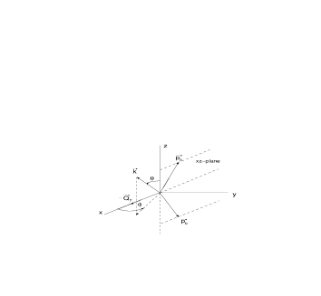
FIG. 4.: Three-momentum kinematics in the DY process for the Collins-Soper frame.

The definition of angles is the same as in [8]. The $W$+jet production is decribed by the transverse momentum $\vec{Q}_{T}$ of the jet and the scattering angle $\hat{\theta}$ in the $W$+jet center of mass frame, $\theta$ and $\phi$ are the polar and the azimuthal angle of the lepton emerging from the decay $W\rightarrow l\nu$ in the Collins-Soper frame [16] as shown in Fig. 4. A simple exercise in particle and parton kinematics shows that the variables $\theta,\phi$ and $\vec{Q}_{T}$ are identical in the hadron and parton processes.

The angular coefficients can be projected from the hadron tensor by means of the Collins-Soper frame projectors

$$P_{7}^{\mu\nu} = \frac{i}{\sqrt{2}q^{2}}\frac{x_{a}x_{b}}{\sqrt{c(1-c)}}(p_{a}^{\mu}p_{b}^{\nu}-p_{a}^{\nu}p_{b}^{\mu}),$$ (127)

$$P_{8}^{\mu\nu} = -\frac{1}{\sqrt{2}q^{4}}\frac{x_{a}^{2}x_{b}^{2}}{c\sqrt{1-c}}[\frac{1}{x_{b}}(p_{a}^{\mu}\epsilon^{\nu\alpha\beta\gamma}p_{a\alpha}p_{b\beta}q_{\gamma}+\mu\leftrightarrow\nu)-\frac{1}{x_{a}}(p_{b}^{\mu}\epsilon^{\nu\alpha\beta\gamma}p_{a\alpha}p_{b\beta}q_{\gamma}+\mu\leftrightarrow\nu)],$$ (128)

$$P_{9}^{\mu\nu} = -\frac{\sqrt{c}}{q^{4}}\frac{x_{a}^{2}x_{b}^{2}}{c(1-c)}[\frac{1}{x_{b}}(p_{a}^{\mu}\epsilon^{\nu\alpha\beta\gamma}p_{a\alpha}p_{b\beta}q_{\gamma}+\mu\leftrightarrow\nu)+\frac{1}{x_{a}}(p_{b}^{\mu}\epsilon^{\nu\alpha\beta\gamma}p_{a\alpha}p_{b\beta}q_{\gamma}+\mu\leftrightarrow\nu)],$$ (129)

which we use to extract the required components $F_{i}$ from the parton level tensor $H_{\mu\nu}$.

Then, taking into account the necessary numerical factors, we have the following relations:

$$K^{-1}f_{7}=\frac{3}{\sqrt{2}}P_{7}^{\mu\nu}H_{\mu\nu} = i\pi\frac{3}{4}\frac{\sqrt{c(1-c)}}{x_{a}x_{b}}H_{5},$$ (130)

$$K^{-1}f_{8}=\frac{3}{2\sqrt{2}}P_{8}^{\mu\nu}H_{\mu\nu} = -i\pi\frac{3}{16}\frac{c\sqrt{1-c}}{x_{a}^{2}x_{b}^{2}}(x_{b}H_{8}-x_{a}H_{9}),$$ (131)

$$K^{-1}f_{9}=-\frac{3}{4}P_{9}^{\mu\nu}H_{\mu\nu} = i\pi\frac{3}{16}\frac{\sqrt{c}(1-c)}{x_{a}^{2}x_{b}^{2}}(x_{b}H_{8}+x_{a}H_{9}),$$ (132)

where $K=8$ for the quark- and antiquark-initiated Compton subprocesses and $K=3$ for the annihilation subprocess. The functions $f_{7},f_{8},f_{9}$ are related to the functions $F_{7}$, $F_{8}$ and $F_{9}$ appearing in eq. (126) and are defined in eqs. (6) and (7) of [8].

Substituting our expressions from (112) and (119) to (130) we find complete agreement with the corresponding results of Eqs. (8) and (9) of ref. [8], except for the sign before the logarithmic term of $f_{A9}$. This typo graphical error was corrected in the footnote of [11] on p. 179.

V Summary and Outlook

Starting from the known one-loop results for the quark-quark-gluon gauge boson four-point function in the $e^{+}e^{-}$-channel [6] we have used analiticity and crossing to derive the absorptive parts of the same four-point function in the DIS channel and in the DY process. Whereas the imaginary parts of the one-loop four-point function generate a nonmeasurable phase in $e^{+}e^{-}$-annihilation one obtains measurable phase effects in DIS and in the DY process leading to the nonvanishing of $T$-odd observables which we have derived. We have compared our results with the results of previous calculations where the absorptive parts in DIS and in the DY process were calculated directly in the respective channels.

In this paper we have mainly considered $T$-odd observables built from triple products of the three-momenta of the respective processes. One can also consider $T$-odd observables built from triple products involving also spins. We have discussed such a triple product observable involving the spin of the initial lepton in DIS. As shown in Sec. III the relevant $T$-odd observable is fed from the parity conserving $T$-odd structure function $H_{5}$ given in this paper. The three absorptive invariant structure functions $H_{5}$, $H_{8}$ and $H_{9}$ presented in this paper suffice to calculate any ${\cal O}(\alpha_{s}^{2})$ contribution to $T$-odd observables as long as the spins of partons or hadrons are summed over. If the $T$-odd triple product involves the spins of hadrons participating in the process the relevant new spin-dependent ${\cal O}(\alpha_{s}^{2})$ contributions can be easily calculated from the absorptive parts of the ${\cal O}(\alpha_{s}^{3/2})$ one-loop amplitudes given in this paper. When one folds these with the respective Born term expressions one has to keep the relevant spins unsummed. We hope to return to the subject of spin-dependent $T$-odd contributions to DIS and the DY process in the future.

A The Triangle Anomaly in DIS

In this Appendix we present the results for the axial-vector part of the quark loop-induced $Zgg$ coupling contribution to DIS. To the best of our knowledge these results have not been presented before. The relevant diagrams and assignments of momenta are shown in Fig. 5.

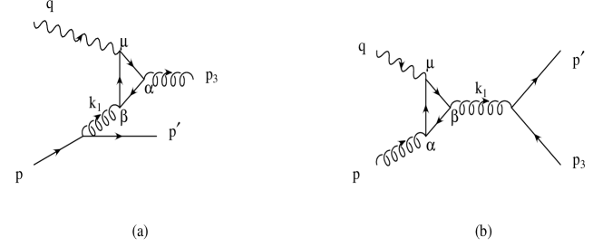
FIG. 5.: Graphs contributing to the $Zgg$ vertex: (a) quark-initiated and (b) gluon-initiated case. Diagrams with counter-clock-wise quarks in the loops are not shown.

We use the results for the $Zgg$ vertex of [11] and apply the above crossing procedure to obtain new results. Following [11], with momentum assignments $Z(q)\rightarrow g(k_{1})+g(k_{2})$ we have the general decomposition for the transition amplitude:

$$T_{\mu\alpha\beta}=f_{1}(k_{2}^{2}\epsilon_{\mu\alpha\beta\rho}k_{1}^{\rho}+k_{2\alpha}\epsilon_{\mu\beta\rho\sigma}k_{2\rho}k_{1\sigma})+f_{2}(k_{1}^{2}\epsilon_{\mu\alpha\beta\rho}k_{2}^{\rho}+k_{1\beta}\epsilon_{\mu\alpha\rho\sigma}k_{2\rho}k_{1\sigma})+$$ (A1)

$$f_{3}(k_{1}+k_{2})_{\mu}\epsilon_{\alpha\beta\rho\sigma}k_{2\rho}k_{1\sigma}+f_{4}(k_{1}-k_{2})_{\mu}\epsilon_{\alpha\beta\rho\sigma}k_{2\rho}k_{1\sigma}),$$ (A2)

where the functions $f_{i}$ depend on the Lorentz scalars $k_{1}^{2},k_{2}^{2}$ and $q^{2}=(k_{1}+k_{2})^{2}$. As the gluon with momentum $k_{2}$ is on shell, $f_{1}$ does not contribute. Due to the property $q_{\mu}L^{\mu\nu}=0$ in the massless lepton limit $f_{3}$ does not contribute. The amplitude $f_{4}$ vanishes identically at the one loop level [17] due to charge conjugation invariance. Technically speaking, the two contributions from the clockwise and counter-clockwise quark flows in the quark loop cancel in $f_{4}$.

Thus, only the term proportional to $f_{2}$ remains. It has to be folded with the Born term amplitude. As it is well known, gauge invariance for the triangle graph with respect to the $Z$-boson momenta is broken. This implies that the squared matrix amplitude can be represented in the form of the decomposition (54) plus additional terms proportional to $q_{\mu}$ or $q_{\nu}$ which, however, do not contribute after folding with the leptonic tensor. Performing the necessary crossing and averaging over initial spins and colors, as defined in Sec. 3, one obtains the anomaly contribution to the DIS structure functions $H_{i}^{q}$. For the quark-initiated case we have:

$$H_{1}^{q} = \frac{4}{3}\frac{x+z}{z}q^{2}{\rm Re}(f_{2}^{q}),$$ (A3)

$$H_{2}^{q} = \frac{8}{3}\frac{x(1+x-z)}{z(1-z)}q^{2}{\rm Re}(f_{2}^{q}),$$ (A4)

$$H_{3}^{q} = \frac{8}{3}\frac{x(1-2x)}{z(1-x)}q^{2}{\rm Re}(f_{2}^{q}),$$ (A5)

$$H_{4}^{q} = -\frac{4}{3}\frac{(1-x)(2-z)-z(1-z)}{\kappa^{2}}q^{2}{\rm Re}(f_{2}^{q}),$$ (A6)

$$H_{6}^{q} = \frac{2}{3}\frac{(1-z)(1-x^{2}+2xz+(1-z)^{2})+x(z-x)}{x\kappa^{2}}q^{2}{\rm Re}(f_{2}^{q}),$$ (A7)

$$H_{7}^{q} = -\frac{2}{3}\frac{(1-z)(2(1-x)(1-2x)+xz)+z^{2}(1-x)}{x\kappa^{2}}q^{2}{\rm Re}(f_{2}^{q}).$$ (A8)

For the antiquark-initiated case results are the same except for $H_{6}^{\bar{q}}=-H_{6}^{q}$ and $H_{7}^{\bar{q}}=-H_{7}^{q}$. Note that there are no absorptive parts in the (anti)quark-initiated case because $f_{2}^{q}$ does not have an imaginary part as we shell see later on.

For the gluon-initiated case we similarly obtain:

$$H_{1}^{g} = -\frac{1-2x}{2(1-x)}q^{2}{\rm Re}(f_{2}^{g}),$$ (A9)

$$H_{2}^{g} = \frac{z(1+x-z)}{\kappa^{2}}q^{2}{\rm Re}(f_{2}^{g}),$$ (A10)

$$H_{3}^{g} = \frac{1}{\kappa^{2}}q^{2}{\rm Re}(f_{2}^{g}),$$ (A11)

$$H_{4}^{g} = -\frac{1-x+2xz}{2\kappa^{2}}q^{2}{\rm Re}(f_{2}^{g}),$$ (A12)

$$H_{5}^{g} = i\frac{x(1-2z)}{2z(1-z)}q^{2}{\rm Im}(f_{2}^{g}),$$ (A13)

$$H_{6}^{g} = -\frac{(1-z)(2x-(1-z)^{2}-(z-x)^{2})-xz(1-x)}{4x\kappa^{2}}q^{2}{\rm Re}(f_{2}^{g}),$$ (A14)

$$H_{7}^{g} = -\frac{1-x-2z(1-z)(1+2x)}{4x\kappa^{2}}q^{2}{\rm Re}(f_{2}^{g}),$$ (A15)

$$H_{8}^{g} = i\frac{xz}{\kappa^{2}}q^{2}{\rm Im}(f_{2}^{g}),$$ (A16)

$$H_{9}^{g} = i\frac{x(1-2z)}{\kappa^{2}}q^{2}{\rm Im}(f_{2}^{g}).$$ (A17)

The functions $f_{2}^{q}$ and $f_{2}^{g}$ can be easily written down using eqs. (2.5)-(2.9) of [11] for the DIS region where $q^{2}<0$. For the (anti)quark-initiated case one also has $k_{1}^{2}<0$. Then we arrive at the following expression for $f_{2}^{q}$:

$$f(w,r)\rightarrow f_{2}^{q}=-\frac{1}{2\pi^{2}q^{2}}\frac{x^{2}}{(x-z)^{2}}\left[\frac{1}{r}\left\{\ln^{2}(\sqrt{1-rw}+\sqrt{-rw})-\ln^{2}(\sqrt{1-r}+\sqrt{-r})\right\}-\right.$$ (A18)

$$\left.2\left\{\sqrt{\frac{1-rw}{-rw}}\ln(\sqrt{1-rw}+\sqrt{-rw})-\sqrt{\frac{1-r}{-r}}\ln(\sqrt{1-r}+\sqrt{-r})\right\}+\ln w\right],$$ (A19)

with $w=k_{1}^{2}/q^{2}$ and $r=q^{2}/4m^{2}$ and where all quark masses are set to zero except for the top quark mass denoted by $m$. This approximation is valid at high enough energies when only the mass of the top quark is important. Then the contributions from the first two generations of ”light” quarks cancel out between the up($u,c$)- and down($d,s$)-quarks and only $b$- and $t$-quarks contribute to the above functions.

One can see that $f_{2}^{q}$ is a real function, and therefore the $T$-odd structure functions in the (anti)quark-initiated case of DIS do not receive any anomaly contribution.

However, for the gluon initiated case we have $k_{1}^{2}>0$, and, clearly, there will be nonvanishing imaginary contribution from the triangle diagram. We have to separately consider the two regions below and above top threshold. Below top threshold with $q^{2}<0,\,\,0<k_{1}^{2}<4m^{2}\,\,(0<rw<1)$ we get:

$${\rm Re}f_{2}^{g} = \frac{x^{2}}{2\pi^{2}q^{2}}\left[\frac{1}{r}\left\{(\sin^{-1}\sqrt{rw})^{2}+\ln^{2}(\sqrt{1-r}+\sqrt{-r})\right\}+\right.$$ (A21)

$$\left.2\left\{\sqrt{\frac{1-rw}{rw}}\sin^{-1}\sqrt{rw}-\sqrt{\frac{1-r}{-r}}\ln(\sqrt{1-r}+\sqrt{-r})\right\}-\ln\mid w\mid\right],$$

$${\rm Im}f_{2}^{g} = \pi$$ (A22)

Since one is below top quark threshold there is only an imaginary part coming from the $b$-quark. The contributions of the ($u,d$) and ($c,s$) quarks cancel pairwise in the real and in the imaginary parts. The $b$-quark contribution in the real part is proportional to the last term in (A21).

Above top threshold with $q^{2}<0,\,\,k_{1}^{2}\geq 4m^{2}\,\,(rw\geq 1)$ we have a $k_{1}^{2}$-dependent imaginary part:

$${\rm Re}f_{2}^{g} = \frac{x^{2}}{2\pi^{2}q^{2}}\left[\frac{1}{r}\left\{\frac{\pi^{2}}{4}-\ln^{2}(\sqrt{rw}+\sqrt{rw-1})+\ln^{2}(\sqrt{1-r}+\sqrt{-r})\right\}+\right.$$ (A24)

$$\left.2\left\{\sqrt{\frac{rw-1}{rw}}\ln(\sqrt{rw}+\sqrt{rw-1})-\sqrt{\frac{1-r}{-r}}\ln(\sqrt{1-r}+\sqrt{-r})\right\}-\ln\mid w\mid\right],$$

$${\rm Im}f_{2}^{g} = \pi\left[1+\frac{1}{r}\ln(\sqrt{rw}+\sqrt{rw-1})-\sqrt{\frac{rw-1}{rw}}\right].$$ (A25)

The trivial imaginary term in (A22) comes entirely from the ”light” $b$-quark contribution. It is also present in (A25), which now also has an imaginary part due to the $t$-quark because now one is above top threshold. In the limit of zero $t$-quark mass the contribution from the triangle graph should vanish. In this case (A21) and (A22) would be obviously absent and, as one can easily see, the real and imaginary contributions in (A24) and (A25) vanish in that limit, serving as a partial check of the correctness of the above expressions.

REFERENCES

[1]
A. de Rujula, R. Petronzio, and B. Lautrup, Nucl. Phys. B146, 50 (1978).
[2]
J. G. Körner, G. Kramer, G. Schierholz, K. Fabricius, and I. Schmitt,
Phys. Lett. 94B, 207 (1980).
[3]
K. Fabricius, I. Schmitt, G. Kramer, and G. Schierholz,
Phys. Rev. Lett. 45, 867 (1980).
[4]
A. Brandenburg, L. Dixon, and Y. Shadmi, Phys. Rev. D53, 1264 (1996).
[5]
K. Hagiwara, K. Hikasa, and N. Kai, Phys. Rev. D27, 84 (1983).
[6]
J. G. Körner and G. Schuler, Z. Phys. C26, 559 (1985).
[7]
K. Hagiwara, K. Hikasa, and N. Kai, Phys. Rev. Lett. 47, 983 (1981).
[8]
K. Hagiwara, K. Hikasa, and N. Kai, Phys. Rev. Lett. 52, 1076 (1984).
[9]
M. Ahmed and T. Gehrmann, Phys. Lett. B465, 297 (1999).
[10]
K. Abe et al. [SLD Collaboration], Phys. Rev. Lett. 75, 4173
(1995);
A. Airapetian et al. [HERMES Collaboration] Phys. Rev. Lett. 84,
4047 (2000).
[11]
K. Hagiwara, T. Kuruma, and Y. Yamada, Nucl. Phys. B369, 171 (1992).
[12]
K. Hagiwara, T. Kuruma, and Y. Yamada, Nucl. Phys. B358, 80 (1991).
[13]
M. Perrottet, Lett. Nuovo Cimento 7, 915 (1973).
[14]
J. G. Körner and P. Sieben, Nucl. Phys. B363, 65 (1991).
[15]
T. Brodkorb and J. G. Körner, Z. Phys. C54, 519 (1992).
[16]
J. C. Collins and D. E. Soper, Phys. Rev. D16, 2219 (1977).