CERN-TH/2000-051

SNS-PH/2000-03

UCD-2000-7

LBNL-45201

Graviscalars from higher-dimensional
metrics and curvature-Higgs mixing

Gian F. Giudice^a, Riccardo Rattazzi^b, James D. Wells^c

^(a)CERN Theory Division, CH-1211 Geneva 23, Switzerland
^(b)INFN and Scuola Normale Superiore, I-56100 Pisa, Italy
^(c)Physics Department, University of California, Davis, CA 95616, USA and
Lawrence Berkeley National Laboratory, Berkeley, CA 94720, USA

We investigate the properties of scalar fields arising from gravity propagating in extra dimensions. In the scenario of large extra dimensions, proposed by Arkani-Hamed, Dimopoulos and Dvali, graviscalar Kaluza-Klein excitations are less important than the spin-2 counterparts in most processes. However, there are important exceptions. The Higgs boson can mix to these particles by coupling to the Ricci scalar. Because of the large number of states involved, this mixing leads, in practice, to a sizeable invisible width for the Higgs. In the Randall-Sundrum scenario, the only graviscalar is the radion. It can be produced copiously at hadron colliders by virtue of its enhanced coupling to two gluons through the trace anomaly of QCD. We study both the production and decay of the radion, and compare it to the Standard Model Higgs boson. Furthermore, we find that radion detectability depends crucially on the curvature-Higgs boson mixing parameter.

hep-ph/0002178

February 2000

1 Introduction

Recently it was recognized that the fundamental scale of quantum gravity could be dramatically lower than the Planck scale provided the Standard Model (SM) fields (gauge bosons and matter) propagate on a 3-dimensional brane and gravity propagates in extra space dimensions. The smallness of Newton’s constant can then be explained by the large size of the volume of compactification, as suggested by Arkani-Hamed, Dimopoulos and Dvali (ADD) [1, 2]. Another possibility, proposed by Randall and Sundrum (RS) [3], is to have a non-factorizable geometry where the 4-dimensional massless graviton wave function is localized away from our brane. If, as motivated by the hierarchy problem, the fundamental gravity scale were not much bigger than a TeV, these scenarios would have distinctive signatures in collider experiments. In the ADD scenario, the production of an essentially continuum spectrum of Kaluza-Klein (KK) graviton excitations gives rise to characteristic missing energy signals [4, 5, 6, 7, 8], while in the RS case one expects to see widely separated and narrow $J=2$ graviton modes [9]. Up to now phenomenological analyses have mainly focused on the production of $J=2$ KK modes, although some studies of the $J=0$ modes have been presented in refs. [6, 10, 11, 12, 13]. (The $J=1$ graviphotons are not coupled at leading order to SM particles). The purpose of this paper is to discuss in detail a few interesting aspects of the phenomenology of graviscalars.

At lowest order, the coupling to gravity waves $h_{AB}$ is

$${\cal L}=-{1\over 2}h_{AB}T^{AB}~{}~{}~{}~{}A=(\mu,i)~{}~{}~{}\mu=0,\dots,3~{}~{}~{}i=4,\dots,D-1,$$ (1)

where $A,B$ run from 0 to $D-1$, while our brane world volume is along $A=\mu$. We expect SM particles to correspond to brane excitations for which the brane itself does not oscillate in the extra dimensions. This means that for processes involving SM particles, $T^{AB}$ has non-zero components only along $A,B=\mu,\nu$. Therefore there is no “direct” coupling to the scalar fields $h_{ij}$, $i,j>3$. However a coupling arises “indirectly” since the scalar $h_{\mu}^{\mu}$ mixes with the $h_{ij}$ in the gravitational kinetic terms. The final result is that $h_{\mu\nu}$ at the brane location includes graviscalars $\varphi_{n}$ when expanded in KK eigenmodes

$$h_{\mu\nu}=\sum_{n}c_{n}\varphi^{(n)}\eta_{\mu\nu}+\left\{J=2~{}{\rm modes}\right\}.$$ (2)

Here $c_{n}$ are effective coupling constants determined by the fundamental gravity scale and by the geometry of compactification. Notice that the general covariance of the full theory constrains these scalars to couple to the trace of the energy-momentum tensor. One such scalar mode is the volume modulus or radion $\varphi^{(0)}$, representing the fluctuations of the compactification volume. Its coupling is $c_{0}=1/M_{P}$, where $M_{P}$ is the ordinary Planck mass in the flat geometry of ADD, while in the RS scenario it is roughly $c_{0}=1/(\Omega M_{P})\sim 1/M_{\rm weak}$, where $\Omega$ is the warp factor. On the other hand, in the models that have been studied so far, the radion is a massless mode and must be stabilized by some mechanism. Therefore the value of the radion mass depends on additional model-building assumptions [14, 15, 16], not just on the geometry.

In the case of 1 extra dimension ($D=5$) the radion is the only scalar mode. One could say that the massive KK excitations of the radion, along with those of the graviphoton, are eaten by the J=2 modes to become massive (a massive $J=2$ graviton has 5 helicity components the same as a massless set of fields $J=0\oplus 1\oplus 2$). For $D>5$ there is, however, a tower of massive KK graviscalars. At each KK level $n$ there is one and only one such scalar $H^{(n)}$ coupled to $T_{\mu}^{\mu}$ [4]. In the flat ADD case all these modes have $c_{n}\sim 1/M_{P}$.

One reason why previous studies have neglected graviscalars is that $T_{\mu}^{\mu}$ vanishes at tree level for massless fermions and massless gauge bosons, which are the quanta colliding in high-energy experiments. For these particles the coupling arises only at 1-loop via the trace anomaly. However things are different, and more interesting, when there are also scalars propagating on the brane. This is because already at the two-derivative level, scalars can couple non-minimally to gravity. This corresponds to the fact that for a scalar $\phi$ one can include in the four-dimensional effective action terms involving the Ricci scalar $R(g)$ of the form

$${\cal L}=MR(g)\phi-\frac{\xi}{2}R(g)\phi^{2}+\cdots.$$ (3)

As is well known, even for a massless scalar, in order to have $T_{\mu}^{\mu}=0$ at tree level one must add the above terms with $M=0$, $\xi=1/6$. For all other choices, a massless scalar would couple to scalar gravitons already at tree level. In the case of the Standard Model Higgs doublet, the gauge symmetry requires $M=0$, but it is difficult to anticipate the precise expected value for the numerical coefficient $\xi$. Naive dimensional analysis suggests $\xi$ to be of order unity. However, if $\phi$ is a Goldstone boson, transforming non-linearly under a symmetry, then $M=0$, $\xi=0$. Therefore, if the Higgs is an approximate Goldstone boson, then we expect a small value of $\xi$.

The most interesting consequence of the terms in eq. (3) is a kinetic mixing between the Higgs and the graviscalar. In the ADD case there is a huge number ${\cal O}(M_{P}^{2})$ of graviton modes, forming a near-continuum sufficiently degenerate in mass with the Higgs boson to allow oscillations. We will show that such oscillations of the Higgs boson into these scalars are equivalent to an invisible decay on collider time scales. This is a generic prediction of theories with large extra dimensions: no quantum number forbids the mixing between the Higgs boson, which lives on the brane, and graviscalars in the bulk. This invisible decay is also quantitatively interesting since, for $m_{h}<2m_{W}$, it competes with the small visible Higgs decay width into $b\bar{b}$.

This paper is organized as follows. In section 2 we concentrate on the large extra dimension case. We recall the properties of the KK scalar gravitons coupled to $T_{\mu}^{\mu}$ and discuss the implications of the operator $\xi R\phi\phi^{\dagger}$. We focus on Higgs-graviton mixing, clarifying why it leads to invisible Higgs decays. We discuss how this invisible channel can compete with the standard visible ones. In section 3 we study the radion phenomenology in the RS scenario, focusing on radion production and decay. In particular we point out the role of the QCD trace anomaly in radion production via gluon fusion.

2 Graviscalars from large extra dimensions

Let us first briefly introduce our notation and recall previously known results. In this section we are considering the case in which the full space-time is $M_{4}\times V_{\delta}$, where $V_{\delta}$ is the large-volume compactified space with $\delta\equiv D-4$ extra dimensions. The action of the theory is given by the $D$-dimensional Einstein term plus a 4-dimensional brane term

$$S=\frac{\bar{M}_{D}^{2+\delta}}{2}\int d^{D}x\sqrt{-g}R+\int d^{4}x\sqrt{-g_{\rm ind}}{\cal L_{\rm sm}}.$$ (4)

Here $\bar{M}_{D}$ is the $D$-dimensional reduced Planck constant and $g_{\rm ind}$ is the induced metric on the brane. For the case of a flat brane we are considering we have simply $(g_{\rm ind})_{\mu\nu}=g_{\mu\nu}$ for $\mu,\nu=$ 0 to 3. Upon integrating eq. (4) over the extra-dimensions we obtain the 4-dimensional reduced Planck mass $\bar{M}_{P}$ [1]

$$\frac{1}{8\pi G_{N}}\equiv\bar{M}_{P}^{2}=\bar{M}_{D}^{2+\delta}V_{\delta}=\bar{M}_{D}^{2+\delta}(2\pi r)^{\delta},$$ (5)

where we have assumed for simplicity that the compactified space with volume $V_{\delta}$ is a $\delta$-torus of radius $r$. If we define for convenience $M_{D}=(2\pi)^{\delta/(2+\delta)}\bar{M}_{D}$ then we can identify

$$M_{D}^{2+\delta}=\bar{M}_{P}^{2}/r^{\delta}.$$ (6)

If $r^{-1}\ll\bar{M}_{P}$ then it is possible to have $M_{D}\ll\bar{M}_{P}$, perhaps as low as the weak scale.

By linearizing $g_{AB}=\eta_{AB}+h_{AB}$ and expanding $h_{AB}$ in Fourier modes

$$h_{AB}=\sum_{n_{1}=-\infty}^{\infty}\cdots\sum_{n_{\delta}=-\infty}^{\infty}\frac{h^{(n)}_{AB}(x)}{\sqrt{V_{\delta}}}e^{in^{j}y_{j}/r},$$ (7)

one finds the physical KK modes [4]. In eq. (7) $y$ are the coordinates of the extra dimensions, and $y=0$ defines the location of our brane. Here we are only interested in the scalar modes living in $h_{\mu\nu}$. (The phenomenology of scalar modes corresponding to brane deformations has been recently considered in ref. [17].) As shown in ref. [4], at each KK level $\vec{n}$ there is only one such mode $H^{(\vec{n})}$ which, after proper normalization, has a lagrangian

$${\cal L} = \sum_{{\rm all}~{}\vec{n}}\left[-\frac{1}{2}H^{(-\vec{n})}(\partial_{\lambda}\partial^{\lambda}+m_{n}^{2})H^{(\vec{n})}+\frac{\kappa}{3\bar{M}_{P}}H^{(\vec{n})}T_{\mu}^{\mu}\right]$$ (8)

$$\kappa \equiv \sqrt{\frac{3(\delta-1)}{\delta+2}}~{}~{}~{}~{}m_{n}^{2}\equiv\frac{\vec{n}^{2}}{r^{2}}.$$ (9)

Notice that the equation above is valid only for $\delta>1$. For $\delta=1$ there are no physical propagating KK graviscalars.

2.1 Scalar-curvature term

The SM energy-momentum tensor is defined as $T^{\mu\nu}=-\eta^{\mu\nu}{\cal L}_{\rm sm}+2\delta{\cal L}_{\rm sm}/\delta g_{\mu\nu}$. However, already at the two-derivative level we can add to ${\cal L}_{\rm sm}$ a term coupling the Higgs field $\phi$ to the Ricci scalar of the induced 4-dimensional metric

$$S=-\xi\int d^{4}x\sqrt{-g_{\rm ind}}R(g_{\rm ind})\phi^{\dagger}\phi.$$ (10)

This term determines an additional effective contribution to $T_{\mu\nu}$ as can be seen by expanding $\sqrt{-g}R$ in the weak gravitational field $g_{\mu\nu}=\eta_{\mu\nu}+h_{\mu\nu}$

$$\sqrt{-g}R=(\partial_{\lambda}\partial^{\lambda}\eta^{\mu\nu}-\partial^{\mu}\partial^{\nu})h_{\mu\nu}(x,y=0)$$ (11)

and taking the variation of eq. (10) with respect to $h_{\mu\nu}$

$$T^{({\rm new})}_{\mu\nu}=T^{({\rm naive})}_{\mu\nu}+2\xi(\eta_{\mu\nu}\partial_{\lambda}\partial^{\lambda}-\partial_{\mu}\partial_{\nu})(\phi^{\dagger}\phi).$$ (12)

The added term is a total derivative and is automatically conserved. The addition of this term to the stress tensor is a standard technicality in field theory in order to “improve” the properties of the dilatation current $S_{\mu}=T_{\mu\nu}x^{\nu}$. In our case, however, since gravity is coupled, the presence of this term has physical consequences. The added term represents a spin-0 field, so on-shell the coupling of the spin-2 graviton KK modes are not affected. The coupling to the scalar KK gravitons $H^{(\vec{n})}$ is crucially changed by the addition $\Delta T_{\mu}^{\mu}=6\xi\hbox{\rule{0.6pt}{7.0pt}\hskip-0.6pt\rule{7.0pt}{0.6pt}\hskip-7.0pt\rule[7.0pt]{7.0pt}{0.6pt}}\rule[7.0pt]{0.6pt}{0.6pt}\hskip-0.6pt\rule{0.6pt}{7.0pt}(\phi\phi^{\dagger})$.

It is clarifying to write ${T^{({\rm new})}}^{\mu}_{\mu}$ in the SM by working in the unitary gauge. Here $\phi$ reduces to the physical real Higgs field $h$, according to $\phi=[(v+h)/{\sqrt{2}},0]$, with $v=246$ GeV. Then, after using the SM equations of motion, we have

$${T^{(\rm new)}}^{\mu}_{\mu} = -(1-6\xi)\left\{\partial_{\mu}h\partial^{\mu}h+M_{V}^{2}V_{A\mu}V_{A}^{\mu}\left(1+\frac{h}{v}\right)^{2}-m_{ij}\bar{\psi}_{i}\psi_{j}\left(1+\frac{h}{v}\right)\right.$$ (13)

$$\left.-\frac{\lambda}{2}\left(v+h\right)^{4}\right\}-(1-3\xi)~{}m_{h}^{2}~{}(v+h)^{2}.$$

Here $V_{A\mu}$ and $\psi_{i}$ are respectively the massive vector bosons and fermions, and we have taken a Higgs potential $V=(\lambda|\phi|^{4}-m_{h}^{2}|\phi|^{2})/2$. Notice that we recovered the standard result that for conformal coupling $\xi=1/6$ the trace is proportional to the truly conformal breaking parameter, the Higgs mass $m_{h}^{2}=\lambda v^{2}$. However for $\xi\not=1/6$, the coupling to the scalar gravitons $H^{(\vec{n})}$ is not suppressed by the Higgs mass. This is manifest for the kinetic and quartic terms of $h$ in eq. (13). It is also true, but less evident, for the massive vector bosons whose coupling is proportional to $M_{V}^{2}\propto m_{h}^{2}$. This is because the wave function for a longitudinally polarized vector at high energy is proportional to the term $p^{\mu}/M_{V}$, which removes the mass suppression in eq. (13). This result is an obvious consequence of the equivalence theorem, by which the vector boson term in eq. (13) can be replaced with the Goldstone boson kinetic term at zeroth order in $g_{\rm weak}$. The results of ref. [6] for the couplings of $H^{(\vec{n})}$ correspond to the choice $\xi=0$. This explains the absence of a $m_{h}^{2}$ (or $M_{V}^{2}$) suppression in the calculated scalar graviton width. However, there is really no good argument to prefer $\xi=0$. For instance, quantum corrections renormalize $\xi$. So it is reasonable to expect $\xi$ to be of order 1. This will be our assumption in the rest of the paper.

A crucial feature of eq. (13) is a linear term in the Higgs field $-6\xi vm_{h}^{2}h$, which is purely generated by the interaction in eq. (10). This term can be read directly from eq. (12), by noticing that $T^{({\rm naive})\mu\nu}=-2\delta{\cal L}_{\rm sm}/\delta g_{\mu\nu}$ is at least quadratic in $h$ on the stationary point of ${\cal L}_{\rm sm}$ and by using the lowest order equation of motion $\hbox{\rule{0.6pt}{7.0pt}\hskip-0.6pt\rule{7.0pt}{0.6pt}\hskip-7.0pt\rule[7.0pt]{7.0pt}{0.6pt}}\rule[7.0pt]{0.6pt}{0.6pt}\hskip-0.6pt\rule{0.6pt}{7.0pt}h=-m_{h}^{2}h$. Because of the interaction in eq. (9), this linear term leads to an $H^{(\vec{n})}$-Higgs mass mixing

$${\cal L}_{\rm mix}=-m^{2}_{\rm mix}h\sum_{\vec{n}}H^{(\vec{n})},~{}~{}~{}~{}m^{2}_{\rm mix}\equiv\frac{2\kappa\xi vm_{h}^{2}}{\bar{M}_{P}}.$$ (14)

In the presence of such mixing, to extract physical information, one would normally try to diagonalize the mass matrix to find the eigenvalues and mixing angles. Here this task is made difficult by the huge number ${\cal O}(M_{P}^{2})$ of graviton levels mixing with $h$. (We recall that the level density around a KK mass $m_{G}$ is $dN=V_{\delta}m_{G}^{\delta-1}dm_{G}/(2\pi)^{\delta}$.) Moreover some of them lie very close to $m_{h}^{2}$ so that perturbation theory would not work. On the other hand, we also do not need all the information contained in the spectrum, as we will never be able to observe a single graviton mode. The information we need can be synthesized into a single expression for the tree level Higgs propagator $G_{h}(p^{2})$

$$\langle hh\rangle_{p^{2}}\equiv G_{h}(p^{2})=\sum_{a}\frac{|U_{a}|^{2}}{p^{2}-m_{a}^{2}+i\epsilon},$$ (15)

where $U_{a}$, $m_{a}$ are the mixing angles and eigenmasses. We can implicitly write $G_{h}$ by formally inverting the mass matrix or, which is the same, by summing up the $m_{\rm mix}^{2}$ insertions. This gives

$$G_{h}(p^{2})=\frac{i}{p^{2}-m^{2}_{h}+\Sigma(p^{2})+i\epsilon},$$ (16)

$$\Sigma(p^{2})\equiv-m^{4}_{\rm mix}\sum_{\vec{n}}\frac{1}{p^{2}-|\vec{n}/r|^{2}+i\epsilon}.$$ (17)

Now, $\Sigma(p^{2})$ is a badly-behaved function (in fact it is a distribution) with singularities at each pole $\vec{n}^{2}/r^{2}$. However, as it is intuitively expected and as we will prove in the sect. 2.2, for observables that do not resolve the single mode the above discrete sum $\sum_{n}$ can be turned into a $d^{\delta}q_{T}$ integral. Then the result becomes quite simple

$$\Sigma(p^{2})\simeq-m_{\rm mix}^{4}\frac{\bar{M}_{P}^{2}}{M_{D}^{2+\delta}}\int\frac{d^{\delta}q_{T}}{p^{2}-q_{T}^{2}+i\epsilon}=\kappa^{2}\xi^{2}S_{\delta-1}\frac{v^{2}m_{h}^{4}}{M^{2+\delta}_{D}}\left[i\pi p^{\delta-2}+F(\Lambda,p^{2})\right].$$ (18)

Here $S_{\delta-1}$ is the surface of a unit-radius sphere in $\delta$ dimensions and $F(\Lambda,p^{2})$ is a cut-off dependent real polynomial of degree $\delta-2$ and $\Lambda$ indicates the cut-off scale at which the effective theory breaks down. $F(\Lambda,p^{2})$, the real part of $\Sigma(p^{2})$, corresponds to a set of local counterterms renormalizing the Higgs pole mass, residue and other input parameters. While these renormalizations have physical consequences, (for instance the wave function renormalization can correct the on-shell higgs couplings by an amount ${\cal O}(m_{h}^{4}/M_{D}^{4})$) they will play no role in our discussion, as it will become clear in a moment. This is in contrast to virtual graviton mediated processes at high-energy colliders, where the value of this function must be hypothesized in order to calculate a rate [4, 6, 18].

As demonstrated above, the function $\Sigma(p^{2})$ has a calculable imaginary part. This can be thought of as a decay of the Higgs into the scalar gravitons $H^{(\vec{n})}$ with partial width

$$\Gamma_{G}=\frac{1}{m_{h}}{\rm Im}\,[\Sigma(p^{2}=m^{2}_{h})]=\pi\kappa^{2}\xi^{2}v^{2}\frac{m_{h}^{1+\delta}}{M_{D}^{2+\delta}}S_{\delta-1}.$$ (19)

This result is quite intuitive, when we think in the $V_{\delta}\rightarrow\infty$ limit. The Higgs excites bulk gravitons via eq. (14), but these escape in the extra-dimension and never come back. So even if $h$ could not decay into any SM particle there would still be no asymptotic Higgs state on the brane because of decay into just one graviton. This is possible because momentum in the direction transverse to the brane is not conserved. This is analogous to the case of the radiative decay of an excited nucleus, in the large-mass limit. In sect. 2.2 we will show that at finite $V_{\delta}$ this decay arises from the overlapping oscillations of the Higgs into the many accessible 4-dimensional $H^{(\vec{n})}$ fields.

Finally, to include the effects of the usual decay modes of the SM Higgs boson we should just add to $\Sigma(p^{2})$ the corresponding one-loop bubble diagrams with the appropriate imaginary parts. We will discuss the phenomenological consequences in sect. 2.3.

2.2 Higgs-graviton mixing: discrete versus continuum

In this section we prove that the mixing to a large number of closely spaced levels is equivalent to a decay. The readers who are already convinced of this assertion and are satisfied with the arguments given in sect. 2.1 may prefer to skip this section.

Consider, for the sake of argument, a close relative to the SM where the Higgs boson is the lightest particle and is stable. The signal of its production is missing energy. For instance, the process $e^{+}e^{-}\rightarrow Zh$ leads to a missing momentum $k^{2}$ delta function at $k^{2}=m_{h}^{2}$. In the presence of the mixing in eq. (14), the missing momentum cross-section for the same reaction will become

$$\frac{d\sigma}{dk^{2}}=\sum_{a}|U_{a}|^{2}\delta(k^{2}-m_{a}^{2})\sigma_{SM}(m_{a}^{2},E).$$ (20)

Here $\sigma_{SM}(m_{a},E)$ is the SM cross section to produce a Higgs of mass $m_{a}$ at center of mass energy $E$, and $d\sigma/dk^{2}$ is a highly discontinuous function that we do not access experimentally when $V_{\delta}\rightarrow\infty$. What we measure experimentally is the convolution

$$\int\frac{d\sigma}{dk^{2}}f(k^{2})dk^{2}$$ (21)

where $f$ is any smooth test function spreading over a finite $k^{2}$ range. For instance, we can imagine the functions $f$ to be of the form

$$f(k^{2})=\frac{C}{((k^{2}-\bar{k}^{2})^{2}+\Gamma^{4})^{n}}$$ (22)

where $\Gamma$ characterizes the width of $f$ around a point $\bar{k}^{2}$. Equation (21), by using eqs. (20) and (15), can be conveniently written as a contour integral

$$\int\frac{d\sigma}{dk^{2}}f(k^{2})dk^{2}\,=\,\oint_{\cal C}\sigma_{SM}(k^{2},E)f(k^{2})G_{h}(k^{2})\frac{dk^{2}}{2\pi i}$$ (23)

where ${\cal C}$ consists of the two lines, one just above and the other just below the real $k^{2}$ axis, oriented as in Fig. 1. The path ${\cal C}$ can be moved away from the real axis, without affecting the result, as long as the poles of $f$ at ${\rm Im}(k^{2})=\pm\Gamma^{2}$ are not crossed. In the limit $V_{\delta}\rightarrow\infty$ the level separation $\Delta m_{G}\sim 1/V_{\delta}$ becomes $\ll\Gamma$, the width of $f$. Now it is convenient to evaluate eq. (23) on a path ${\cal C}_{\bar{\epsilon}}$ defined by ${\rm Im}k^{2}=\pm\bar{\epsilon}$ with $\Delta m_{G}^{2}\ll\bar{\epsilon}\ll\Gamma^{2}$. On ${\cal C}_{\bar{\epsilon}}$ we can still approximate $\sigma(k^{2}\pm i\bar{\epsilon})\simeq\sigma(k^{2})$ and $f(k^{2}+i\bar{\epsilon})\simeq f(k^{2})$. Moreover, since $\Delta m_{G}^{2}\ll\bar{\epsilon}$, the discrete sum defining $G_{h}$ in eqs. (16, 17) involves a function $(k^{2}-m_{n}^{2}+i\bar{\epsilon})^{-1}$ which is no longer rapidly varying from mode to mode. Therefore we can safely convert the sum to an integral

$${1\over V_{\delta}}\sum_{n}\frac{1}{k^{2}-(n/r)^{2}+i\bar{\epsilon}}=\int\frac{d^{\delta}q_{T}}{k^{2}-q_{T}^{2}+i\bar{\epsilon}}+{\cal O}\left(\frac{1}{V_{\delta}\bar{\epsilon}}\right)$$ (24)

where $i\bar{\epsilon}$ plays now the role of the usual $i\epsilon$. We conclude that for $V_{\delta}\bar{\epsilon}\sim\bar{\epsilon}/\Delta m_{G}^{2}\rightarrow\infty$, $\Sigma(p^{2})$ can be replaced by the continuum limit in eq. (18) and the integral over ${\cal C}_{\bar{\epsilon}}$ reduces to

$$\int\frac{d\sigma}{dk^{2}}f(k^{2})dk^{2}\simeq\frac{1}{\pi}\int\sigma_{SM}(k^{2},E)f(k^{2})\frac{m_{h}\Gamma_{G}}{(k^{2}-m_{h}^{2})^{2}+m_{h}^{2}\Gamma_{G}^{2}}{dk^{2}}$$ (25)

This is the usual Breit-Wigner formula for a resonance of width $\Gamma_{G}$, where $\Gamma_{G}$ is given in eq. (19). Technically what we have shown is that the distribution in eq. (20) when acting on a smooth function can be replaced with a continuous Breit-Wigner function. The essential ingredient in the simplification of the final expression is that it represents an inclusive quantity over all the modes that for $V_{\delta}\rightarrow\infty$ become degenerate with the Higgs. On the other hand, exclusive quantities, representing the production of individual modes, do not have a smooth $V_{\delta}\rightarrow\infty$ limit.

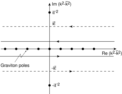
Figure 1: The contour of integration ${\cal C}$ (solid line) and ${\cal C}_{\bar{\epsilon}}$ (dashed line) in the $k^{2}-{\bar{k}}^{2}$ complex plane. It is assumed that $\Delta m_{G}^{2}\ll\bar{\epsilon}\ll\Gamma^{2}$, where $\Delta m_{G}^{2}$ is the splitting between graviton poles.

The Higgs-graviton mixing we are considering should be contrasted to the case of a mixing between the SM left-handed neutrinos and fermions living in the bulk [19, 20]. The resulting neutrino mass is practically zero (it is indeed a $1/M_{P}$ effect), so the KK level density that it experiences is very small and only a few levels mix significantly. So the appropriate description is in terms of usual mixing. Indeed, also in our case the mixing looks like a decay only as long as $\Gamma_{G}$ is much bigger than the separation of KK levels, i.e. as long as $m_{h}^{\delta}\gg M_{D}^{2+\delta}/(vM_{P})$, see eq. (19).

It is instructive to present another point of view on the Higgs-graviton mixing based on time oscillations. Let us work in the non-relativistic limit to simplify notation. Because of eq. (15), we can write the Higgs state as a sum over the mass eigenstates

$$|h\rangle=\sum_{a}U_{a}|a\rangle.$$ (26)

The $|h\rangle$ to $|h\rangle$ amplitude at time $t$ is

$$A(t)=\langle h(t)|h(0)\rangle=\sum_{a}e^{-im_{a}t}|U_{a}|^{2}.$$ (27)

If we want to study the behavior of $A(t)$ for times $t\ll 1/\Delta m_{G}$, for which the graviton levels cannot be resolved, then we should consider the Fourier (Laplace) transform

$$\hat{A}(\omega)=\int_{0}^{\infty}e^{i(\omega+i\bar{\epsilon})t}A(t)=\sum_{a}\frac{1}{\omega-m_{a}+i\bar{\epsilon}}|U_{a}|^{2}$$ (28)

where $\bar{\epsilon}$ is taken to be much bigger than $\Delta m_{G}$ but much smaller than any laboratory energy or inverse time. As was the case before, $(\omega-m_{a}+i\bar{\epsilon})^{-1}$ is now a smooth function of $m_{a}$, and we can safely convert the sum to an integral. Therefore, with the proper normalization, eq. (28) reduces to the non-relativistic limit of eq. (16), with $\Sigma$ given by the continuum limit eq. (18)

$$\hat{A}(\omega)=\frac{1}{\omega-m_{h}+i\Gamma_{G}/2}.$$ (29)

So even though at times $t>1/\Delta m_{G}$, the amplitude $A(t)$ may display a complicated oscillation pattern reflecting the structure of the graviton spectrum, at times $\ll 1/\Delta m_{G}$ the various oscillation amplitudes sum up to give an exponential decay $|A|\sim{\rm exp}(-t\Gamma_{G}/2)$.

2.3 Invisible Higgs width

The partial width $\Gamma_{G}$ contributes to the invisible width of the Higgs since the $H^{(\vec{n})}$ will not interact with the detector or decay inside. The Higgs boson also has visible decay modes in the SM that will compete with this invisible partial width. For Higgs bosons with mass below about $150\hbox{\rm\,GeV}$ the total width into SM states is less than $20\hbox{\rm\,MeV}$. This is extremely narrow, and so any new decay modes may likely dominate over SM modes. Above the $h\rightarrow WW$ threshold, the total width is unsuppressed and so new decay modes are not likely to dominate, but can compete with SM states at best.

In Fig. 2 we plot the branching fraction of the Higgs boson to decay invisibly,

$$B(h\rightarrow{\rm invisible})=\frac{\Gamma_{G}}{\Gamma_{\rm SM}+\Gamma_{G}}.$$ (30)

The plot is made for $M_{D}=2\hbox{\rm\,TeV}$, $\xi=1$, and for various numbers of extra dimensions $\delta$. The scaling with respect to these parameters can be obtained from eq. (19).

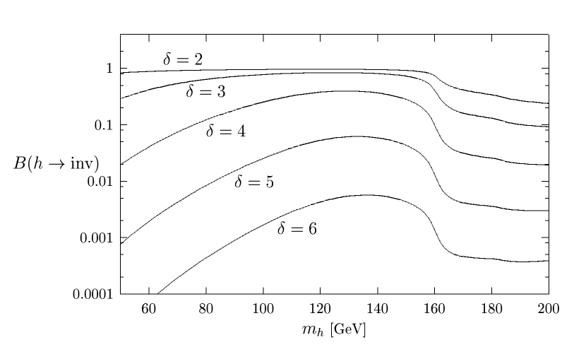
Figure 2: Branching fraction of the Higgs boson to decay invisibly as a function of its mass, for $M_{D}=2\hbox{\rm\,TeV}$ and $\xi=1$. The rapid decrease at $m_{h}\simeq 160\hbox{\rm\,GeV}$ is due to the onset of $h\rightarrow WW$ on-shell decays.

At LEP2, the invisible decaying Higgs boson has been searched for by all four collaborations [21]. No evidence has been found for this state, and the lower limit on the mass of a Higgs boson with SM production cross section and 100% invisible branching ratio is now 98.9 GeV. Future analyses with $\sqrt{s}\simeq 200\hbox{\rm\,GeV}$ are expected to either find the invisible Higgs boson or exclude its existence up to nearly $105\hbox{\rm\,GeV}$.

At the Tevatron with $30\hbox{\rm\, fb}^{-1}$ of integrated luminosity, an invisibly decaying Higgs boson could be discovered at greater than $5\sigma$ significance if its mass is below $110\hbox{\rm\,GeV}$, and it could be excluded at the 95% C.L. if its mass is less than $145\hbox{\rm\,GeV}$ [22]. At the LHC, searches are likely to find evidence for such a Higgs boson if its mass is below about $250\hbox{\rm\,GeV}$ [23].

It is conceivable that a future muon collider working around the Higgs resonance will be capable of measuring the Higgs total width $\Gamma^{\rm tot}_{h}$ to a precision better than 20% in the mass range $110\hbox{\rm\,GeV}\lower 3.01385pt\hbox{$\;\stackrel{{\scriptstyle\textstyle<}}{{\sim}}\;$}m_{h}\lower 3.01385pt\hbox{$\;\stackrel{{\scriptstyle\textstyle<}}{{\sim}}\;$}150\hbox{\rm\,GeV}$ [24, 25]. Combining high luminosity $e^{+}e^{-}$ collider data ($500\hbox{\rm\,GeV}$ with $200\hbox{\rm\, fb}^{-1}$) with muon collider data (on-shell scan of $0.4\hbox{\rm\, fb}^{-1}$), it is reasonable to expect better than 12% total width determination in the mass range $80\hbox{\rm\,GeV}<m_{h}<170\hbox{\rm\,GeV}$ [26]. We assume that the sensitivity to $\Gamma_{G}$ will be close to the ability to determine the width, $\Delta\Gamma_{h}^{\rm tot}$. This in turn implies that the sensitivity to $M_{D}$ is

$$M_{D}<\left[\frac{\pi\kappa^{2}\xi^{2}v^{2}m^{\delta+1}_{h}S_{\delta-1}}{\Delta\Gamma_{h}^{\rm tot}}\right]^{\frac{1}{\delta+2}}.$$ (31)

In Fig. 3 we plot these sensitivity limits, using $\Delta\Gamma_{h}^{\rm tot}$ values from ref. [26] as a function of $m_{h}$ for different numbers of extra dimensions, and for $\xi=1$. One can scale the result easily for other values of $\xi$ according to the above equation. We can see that the sensitivity to $M_{D}$ is best for lower numbers of extra dimensions as is usually the case because the phase space density of “light” KK modes is higher with fewer dimensions.

Figure 3: Upper bound on the sensitivity to $M_{D}$ from invisible width measurements of the Higgs boson. We have approximated the width measurement capability as the expected uncertainty in the SM Higgs width determination [26] at a muon collider (on-shell scan with $0.4\hbox{\rm\, fb}^{-1}$) and $e^{+}e^{-}$ linear collider ($\sqrt{s}=500\hbox{\rm\,GeV}$ with $200\hbox{\rm\, fb}^{-1}$) given $\xi=1$ and various choices of the number of extra dimensions $\delta$.

An invisibly decaying Higgs boson is not necessarily evidence for Higgs boson oscillations into graviscalars. There are many extensions of the SM that predict the Higgs boson decaying into undetectable states (see e.g. ref. [22]). For example, Higgs decays into singlet scalars or Majorons are just two four-dimensional examples of an invisible partial width. Furthermore, there are other intrinsically extra-dimensional decays beyond the decays to graviscalars. If the right-handed neutrino lives in the bulk, Higgs decays into all accessible neutrino pairs can have an ${\cal O}(1)$ branching fraction [19, 22]. Distinguishing between these possibilities is extremely difficult without additional observables. Nevertheless, the effects do cause deviations from SM expectations, and so it is meaningful to speak of sensititivity to $M_{D}$ in these theories. Although dependent on unknown parameters such as $\xi$ and $\delta$, the multi-TeV sensitivity to $M_{D}$ that we have demonstrated in the analysis for next generation colliders, such as the LHC and a muon collider, compares favorably with sensitivities derived from calculable external KK spin-2 graviton processes [4, 5].

2.4 Direct graviscalar production at LEP2

In the previous section we discussed effects of graviscalars on the invisible width of the Higgs boson. One can also search for graviscalars in direct production at high-energy colliders. Earlier we suggested that spin-0 KK effects were usually not as relevant to direct collider physics probes/constraints as the spin-2 KK effects, because they couple only to the trace of the energy-momentum tensor. At very high-energy scattering in hadron colliders, they can be produced by gluon fusion, but their production is suppressed with respect to spin-2 gravitons by a loop factor in the amplitude. Production through $W$ fusion is subleading. However, for colliders running at energies not much above $M_{Z}$, it is possible that external spin-0 KK production could impact collider observables.

The graviscalar coupling to heavy gauge bosons is most relevant for $e^{+}e^{-}$ colliders working at energies not much larger than $M_{Z}$, as in the case of LEP2. The inclusive differential cross section for graviscalars accompanied by a $Z$ boson is given by

$$\frac{d\sigma(e^{+}e^{-}\rightarrow ZH^{(\vec{n})})}{dM_{\rm miss}} = \frac{G_{F}~{}M_{Z}^{4}~{}\kappa^{2}~{}S_{\delta-1}~{}|1-6\hat{\xi}|^{2}~{}M_{\rm miss}^{\delta-1}}{432\sqrt{2}\pi~{}s~{}M_{D}^{\delta+2}}\left(1-4\sin^{2}\theta_{W}+8\sin^{4}\theta_{W}\right)$$ (32)

$$\times f\left(\frac{M_{\rm miss}^{2}}{s},\frac{M_{Z}^{2}}{s}\right),$$ (33)

where

$$\hat{\xi} = \frac{\xi M^{2}_{\rm miss}}{M^{2}_{\rm miss}-m^{2}_{h}+i\Gamma_{h}m_{h}},$$ (34)

$$f(x,y) = \frac{(1-x)^{2}+y(y-2x+10)}{(1-y)^{2}}\sqrt{(1-x)^{2}+y(y-2x-2)},$$ (35)

and $M_{\rm miss}$ represents the graviscalar mass. Because there is a near-continous tower of KK masses for the graviscalars, a continuous distribution in $M_{\rm miss}$ results.

Notice that in the limit $m_{h}\rightarrow\infty$ the cross section becomes $\xi$ independent. In this limit the only scalars on the brane are the eaten Goldstones. Then the result is consistent with the fact that no mixing to the Ricci tensor can be written for Goldstone bosons (they couple minimally to gravity). On the other hand, for $m_{h}\ll M_{\rm miss}$ the cross section is proportional to $1-6\xi$. This corresponds to the high energy limit of a linear Higgs model, where the Higgs and the Goldstones behave similarly. For $M_{\rm miss}\simeq m_{h}$ the above expression is dominated by the production of a real Higgs that decays into invisible graviscalars. This is the process we discussed in the previous section.

In Fig. 4 we plot the total differential cross-section as a function of $M_{\rm miss}$ for LEP2 running at $\sqrt{s}=200\hbox{\rm\,GeV}$ center of mass energy. For this plot we have chosen $M_{D}=1\hbox{\rm\,TeV}$ and $\xi=0$. For different choices of these parameters one should rescale the curves by,

$${\rm Rescale~{}factor~{}}=|1-6\hat{\xi}|^{2}\left(\frac{1\hbox{\rm\,TeV}}{M_{D}}\right)^{2+\delta}.$$ (36)

The maximal integrated luminosity at LEP2 running above $\sqrt{s}=200\hbox{\rm\,GeV}$ is not expected to exceed $1\hbox{\rm\, fb}^{-1}$, summing over the four detectors. Obtaining even a few total events of $e^{+}e^{-}\rightarrow ZH^{(\vec{n})}$ at LEP2 requires a large rescaling factor. That is, $M_{D}$ needs to be substantially below $1\hbox{\rm\,TeV}$ or $\hat{\xi}$ must be substantially above 1 in order to produce a few events. Filling out a signal distribution in the missing mass spectrum of $Z+{\rm invisible}$ events at LEP2 requires an even higher enhancement factor. The expected background for these events can be found in ref. [21]. The missing mass spectrum is peaked at $M_{Z}$, and the total selected event rate with $Z\rightarrow q\bar{q}$ corresponds to approximately 25 events in a 7 GeV mass bin centered on $M_{Z}$ for $\sqrt{s}=189\hbox{\rm\,GeV}$ (see the DELPHI article in ref. [21]).

Figure 4: Differential signal cross-section of $e^{+}e^{-}\rightarrow ZH^{(\vec{n})}$ at LEP2 with $200\hbox{\rm\,GeV}$ center of mass energy and for the parameter choices $M_{D}=1\hbox{\rm\,TeV}$ and $\xi=0$. $M_{\rm miss}$ is the missing mass associated with escaping graviscalars.

In contrast, the production rate for spin-2 KK excitations in association with photons and Z is much higher for the same parameter values [4]. With a total of $2\hbox{\rm\, fb}^{-1}$, $M_{D}$ can be probed above $1.3\hbox{\rm\,TeV}$ in the $\gamma+$ missing energy signature alone for $\delta=2$. For these reasons we conclude that KK graviscalar direct production at colliders is not likely to be as probing as KK graviton direct production. Nevertheless, the conclusions of the previous subsection still hold. If the Higgs boson is kinematically accessible, there can also be a resonant missing energy contribution coming from the graviscalar-Higgs mixing, which is described by the Higgs invisible width in eq. (19). This effect could be the earliest signal of extra dimensions at colliders.

3 Graviscalars from non-factorizable geometries

In this section we discuss the phenomenology of the radion in the scenario of Randall-Sundrum [3]. The extra dimensional space is now a $S^{1}/Z_{2}$ orbifold parametrized by a coordinate $y\in[-\pi,\pi]$. The geometry is the same as a slice of $AdS_{5}$

$$ds^{2}=e^{-2kr_{c}|y|}\eta_{\mu\nu}dx^{\mu}dx^{\nu}-r_{c}^{2}dy^{2}.$$ (37)

where $1/k$ is the $AdS$ curvature radius and $r_{c}$ is the volume radius. The above metric solves Einstein’s equations with a negative bulk cosmological constant and in the presence of two branes at $y=0$ and $y=\pi$ with respectively positive and negative tensions. A field theory living on the $y=\pi$ brane experiences an exponential red-shift $e^{-kr_{c}\pi}$ of all its mass parameters with respect to a theory living at $y=0$. If one assumes that the SM lives at $y=\pi$, then it is enough to have $kr_{c}\pi\sim 35$ to explain the hierarchy between $M_{\rm weak}/M_{P}$ in a natural way. This fact motivates the great interest in this scenario.

The above metric admits two types of massless excitations described by $\eta_{\mu\nu}\rightarrow g_{\mu\nu}(x)$, the usual 4-d graviton, and by $r_{c}\rightarrow T(x)$, the radion. In terms of these two dynamical fields, the metric can be recast in the form,

$$ds^{2}=e^{-2k|y|T(x)}g_{\mu\nu}(x)dx^{\mu}dx^{\nu}-T^{2}(x)dy^{2}.$$ (38)

Of course in order to avoid violations of the equivalence principle the modulus $T$ must acquire a mass. A mechanism that stabilizes $T$ should also explain why its vacuum expectation value $\langle T(x)\rangle=r_{c}$ is somewhat larger than the $AdS$ radius: $r_{c}\sim 11/k$. Indeed Goldberger and Wise (GW) [16] have found a nice mechanism with these features. One consequence of the GW mechanism is that in order to have $k\pi r_{c}\sim 35$ the radion should be somewhat lighter than the $J=2$ KK excitations. The radion is therefore likely to be the first state experimentally accessible in this scenario.

To write down the effective $3+1$ dimensional theory it is more convenient to express the radion field in terms of the field $\varphi$ defined by

$$\varphi\equiv\Lambda_{\varphi}e^{-k\pi(T-r_{c})},~{}~{}~{}~{}\Lambda_{\varphi}\equiv\langle\varphi\rangle=\sqrt{\frac{24M_{5}^{3}}{k}}e^{-k\pi r_{c}},$$ (39)

where $M_{5}$ is the Planck scale of the fundamental 5-dimensional theory. Integrating over the orbifold coordinate one then gets a canonically normalized effective action [10, 11]

$$S_{\varphi}=\int d^{4}x\sqrt{-g}\left[\frac{2M_{5}^{3}}{k}\left(1-\frac{\varphi^{2}}{\Lambda_{\varphi}^{2}}e^{-2k\pi r_{c}}\right)R+\frac{1}{2}\partial_{\mu}\varphi\partial^{\mu}\varphi-V(\varphi)+\left(1-\frac{\varphi}{\Lambda_{\varphi}}\right)T^{\mu}_{\mu}\right].$$ (40)

Here $V(\varphi)$ is the potential which stabilizes the radion field $\varphi$. For phenomenological purposes, we are interested only in $T_{\mu}^{\mu}$ terms that are at most bilinear in the SM fields. These are given by

$${T^{(1)}}^{\mu}_{\mu}=6\xi v\hbox{\rule{0.6pt}{7.0pt}\hskip-0.6pt\rule{7.0pt}{0.6pt}\hskip-7.0pt\rule[7.0pt]{7.0pt}{0.6pt}}\rule[7.0pt]{0.6pt}{0.6pt}\hskip-0.6pt\rule{0.6pt}{7.0pt}h,$$ (41)

$${T^{(2)}}^{\mu}_{\mu}=(6\xi-1)\partial_{\mu}h\partial^{\mu}h+6\xi h\hbox{\rule{0.6pt}{7.0pt}\hskip-0.6pt\rule{7.0pt}{0.6pt}\hskip-7.0pt\rule[7.0pt]{7.0pt}{0.6pt}}\rule[7.0pt]{0.6pt}{0.6pt}\hskip-0.6pt\rule{0.6pt}{7.0pt}h+2m_{h}^{2}h^{2}+m_{ij}\bar{\psi}_{i}\psi_{j}-M_{V}^{2}V_{A\mu}V_{A}^{\mu}.$$ (42)

Equations (41) and (42) reduce to eq. (13) after using the equations of motion for the matter fields, up to terms containing three or more fields.

The existence of ${T^{(1)}}^{\mu}_{\mu}$ induces a kinetic mixing between $\varphi$ and $h$. After shifting $\varphi$ by its vacuum expectation value $\langle\varphi\rangle=\Lambda_{\varphi}$, the lagrangian containing bilinear terms in $\varphi$ and $h$ is given by

$${\cal L}=-\frac{1}{2}\varphi\left(\hbox{\rule{0.6pt}{7.0pt}\hskip-0.6pt\rule{7.0pt}{0.6pt}\hskip-7.0pt\rule[7.0pt]{7.0pt}{0.6pt}}\rule[7.0pt]{0.6pt}{0.6pt}\hskip-0.6pt\rule{0.6pt}{7.0pt}+m_{\varphi}^{2}\right)\varphi-\frac{1}{2}h\left(\hbox{\rule{0.6pt}{7.0pt}\hskip-0.6pt\rule{7.0pt}{0.6pt}\hskip-7.0pt\rule[7.0pt]{7.0pt}{0.6pt}}\rule[7.0pt]{0.6pt}{0.6pt}\hskip-0.6pt\rule{0.6pt}{7.0pt}+m_{h}^{2}\right)h-\frac{6\xi v}{\Lambda_{\varphi}}\varphi\hbox{\rule{0.6pt}{7.0pt}\hskip-0.6pt\rule{7.0pt}{0.6pt}\hskip-7.0pt\rule[7.0pt]{7.0pt}{0.6pt}}\rule[7.0pt]{0.6pt}{0.6pt}\hskip-0.6pt\rule{0.6pt}{7.0pt}h.$$ (43)

Here $m_{\varphi}$ is the mass parameter contained in $V(\varphi)$. This lagrangian can be diagonalized by the field redefinitions

$$\varphi=\left(\sin\theta-\sin\rho\cos\theta\right)h^{\prime}+\left(\cos\theta+\sin\rho\sin\theta\right)\varphi^{\prime},$$ (44)

$$h=\cos\rho\cos\theta~{}h^{\prime}-\cos\rho\sin\theta~{}\varphi^{\prime},$$ (45)

$$\tan\rho\equiv\frac{6\xi v}{\Lambda_{\varphi}},~{}~{}~{}\tan 2\theta\equiv\frac{2\sin\rho~{}m_{\varphi}^{2}}{\cos^{2}\rho(m_{\varphi}^{2}-m_{h}^{2})}.$$ (46)

The new fields $\varphi^{\prime}$ and $h^{\prime}$ are mass eigenstates with eigenvalues

$$m^{2}_{\varphi^{\prime},h^{\prime}}=\frac{1}{2}\left[(1+\sin^{2}\rho)m_{\varphi}^{2}+\cos^{2}\rho~{}m_{h}^{2}\pm\sqrt{\cos^{4}\rho(m_{\varphi}^{2}-m_{h}^{2})^{2}+4\sin^{2}\rho~{}m_{\varphi}^{4}}\right].$$ (47)

Since we are dealing with an effective theory that contains higher-dimensional operators suppressed by inverse powers of $\Lambda_{\varphi}$, in the following we will often expand eqs. (44)–(47) and keep only the leading terms in $1/\Lambda_{\varphi}$. Notice that, if $m_{\varphi}^{2}-m_{h}^{2}$ is small, one should retain higher orders in the expression of the mixing angle $\theta$.

3.1 Radion interactions with matter

The interaction of the fields $\varphi$ and $h$ with fermions and massive gauge bosons is given by

$${\cal L}=-\frac{1}{v}\left(m_{ij}\bar{\psi}_{i}\psi_{j}-M_{V}^{2}V_{A\mu}V_{A}^{\mu}\right)\left[h+\frac{v}{\Lambda_{\varphi}}\varphi\right].$$ (48)

From this, we can obtain the interaction terms for the mass eigenstates $\varphi^{\prime}$ and $h^{\prime}$ by substituting eqs. (44) and (45) into eq. (48). We find that the radion decay widths into two fermions and two massive gauge bosons are given by

$$\frac{\Gamma(\varphi^{\prime}\rightarrow\bar{f}f,WW,ZZ)}{\Gamma(h_{\rm sm}\rightarrow\bar{f}f,WW,ZZ)}=\frac{v^{2}}{\Lambda^{2}_{\varphi}}(a_{1}-a_{2})^{2},$$ (49)

$$a_{1}=\cos\theta+\sin\rho\sin\theta,~{}~{}~{}~{}{\rm and}~{}~{}~{}~{}~{}~{}a_{2}=\frac{\Lambda_{\varphi}}{v}\cos\rho\sin\theta.$$ (50)

Here $\Gamma(h_{\rm sm}\rightarrow\bar{f}f,WW,ZZ)$ are the usual decay widths of the SM Higgs boson with $m_{h_{\rm sm}}=m_{\varphi^{\prime}}$. Expanding at leading order in $1/\Lambda_{\varphi}$, we find

$$a_{1}-a_{2}=\left(1-\frac{6\xi m_{\varphi}^{2}}{m_{\varphi}^{2}-m_{h}^{2}}\right)+{\cal O}\left(\frac{1}{\Lambda_{\varphi}}\right).$$ (51)

Notice that eq. (51) vanishes in the conformal limit $m_{h}=0$, $\xi=1/6$. The term proportional to $\xi$ in eq. (51) can also be understood in a diagrammatic fashion as a Higgs-radion insertion on a Higgs-matter coupling.

The coupling of the radion to two Higgs bosons is not model-independent because it can be affected by the stabilizing potential $V(\varphi)$ after the field redefinitions in eqs. (44) and (45). If we assume that the radion self-couplings in $V(\varphi)$ are small, then the decay width of the radion into two Higgs bosons is determined by the interactions in eq. (40),

$$\Gamma(\varphi^{\prime}\rightarrow h^{\prime}h^{\prime})=\frac{m_{\varphi^{\prime}}^{3}}{32\pi\Lambda_{\varphi}^{2}}\left[1-6\xi+2\frac{m_{h^{\prime}}^{2}}{m_{\varphi^{\prime}}^{2}}(1+6\xi)\right]^{2}\sqrt{1-4\frac{m_{h^{\prime}}^{2}}{m_{\varphi^{\prime}}^{2}}},$$ (52)

at leading order in $1/\Lambda_{\varphi}$. Again, the width vanishes in the conformal limit.

The production of both Higgs and radion fields at hadron colliders, in the mass range of interest, is dominated by gluon-gluon fusion. The effective vertex at momentum transfer $q$ along the scalar line is given by

$$\left[{\varphi\over\Lambda_{\varphi}}b_{3}-\frac{1}{2}\left({\varphi\over\Lambda_{\varphi}}+{h\over v}\right)F_{1/2}(\tau_{t})\right]\frac{\alpha_{s}}{8\pi}G_{\mu\nu}G^{\mu\nu},$$ (53)

where $\tau_{t}=4m^{2}_{t}/q^{2}$, and $F_{1/2}$ is given in the appendix. We identify $q^{2}=m_{\varphi^{\prime}}^{2}$ when we calculate the on-shell decays of $\varphi^{\prime}\rightarrow gg$.

The first term in eq. (53), where $b_{3}=7$ is the QCD $\beta$-function coefficient in the SM, represents the QCD trace anomaly. The second term originates from 1-loop diagrams involving virtual top quarks. The form factor $F_{1/2}(\tau_{t})$ is such that $F_{1/2}\rightarrow-4/3$ for $\tau\rightarrow\infty$, and $F_{1/2}\rightarrow 0$ for $\tau\rightarrow 0$. Notice that for $m_{t}^{2}\gg q^{2}$, the coupling to $\varphi$ becomes proportional to the $\beta$-function for 5-flavors $b_{3}+2/3$, consistent with top decoupling. By substituting eqs. (44) and (45) into eq. (53) we obtain the $gg$ coupling to the mass eigenstates $h^{\prime}$, $\varphi^{\prime}$. The decay width of the radion into two gluons is given by

$$\frac{\Gamma(\varphi^{\prime}\rightarrow gg)}{\Gamma(h_{\rm sm}\rightarrow gg)}=\frac{v^{2}}{\Lambda^{2}_{\varphi}}\frac{|2a_{1}b_{3}-(a_{1}-a_{2})F_{1/2}(\tau_{t})|^{2}}{|F_{1/2}(\tau_{t})|^{2}},$$ (54)

where $a_{1}$ and $a_{2}$ are given in eq. (50).

A similar expression describes the coupling to two photons

$$\left\{{\varphi\over\Lambda_{\varphi}}\left(b_{2}+b_{Y}\right)-\left({\varphi\over\Lambda_{\varphi}}+{h\over v}\right)\left(F_{1}(\tau_{W})+\frac{4}{3}F_{1/2}(\tau_{t})\right)\right\}\frac{\alpha_{EM}}{8\pi}F_{\mu\nu}F^{\mu\nu},$$ (55)

where $F_{1}(\tau_{W})$ is a form factor from the loop with virtual $W$’s (see appendix), while $b_{2}=19/6$ and $b_{Y}=-41/6$ are the SM $SU(2)\times U(1)_{Y}$ $\beta$-funtion coefficients. At $m_{t}^{2}/q^{2}\rightarrow\infty$ the coupling to $\varphi$ reduces to the QED $\beta$-function with $e,\mu,\tau$ and $u,d,s,c,b$

$$b_{2}+b_{Y}-F_{1}(\infty)-\frac{4}{3}F_{1/2}(\infty)=-\frac{80}{9}=b_{\rm QED},$$ (56)

demonstrating again the correct decoupling behavior for heavy top quark and $W$ boson. The decay width of the radion into two photons is

$$\frac{\Gamma(\varphi^{\prime}\rightarrow\gamma\gamma)}{\Gamma(h_{\rm sm}\rightarrow\gamma\gamma)}=\frac{v^{2}}{\Lambda^{2}_{\varphi}}\frac{|3a_{1}(b_{Y}+b_{2})-(a_{1}-a_{2})(4F_{1/2}(\tau_{t})+3F_{1}(\tau_{W}))|^{2}}{|4F_{1/2}(\tau_{t})+3F_{1}(\tau_{W})|^{2}}.$$ (57)

3.2 Radion branching fractions and production

In this section we will compute the decay branching fractions and production cross-sections of the radion. An accurate computation of the radion partial widths is best performed by rescaling well-known SM Higgs boson partial widths [27] according to the formulae of the previous section. Since we will encounter regions of parameter space where mixing between the radion $\varphi$ and Higgs boson $h$ is large, we must specify which state we choose to call the radion mass eigenstate $\varphi^{\prime}$ and which state we call the Higgs mass eigenstate $h^{\prime}$. Our convention is to identify the radion mass eigenstate with the lighter of the two solutions of eq. (47) if $m_{\varphi}<m_{h}$, and the heavier of the two solutions if $m_{\varphi}>m_{h}$.

In Fig. 5 we plot the branching fractions of the radion mass eigenstate as a function of its mass for $\Lambda_{\varphi}=10\hbox{\rm\,TeV}$, $m_{h}=125\hbox{\rm\,GeV}$ and $\xi=0$. Fig. 5a shows the branching fraction over the light mass range of $50\hbox{\rm\,GeV}$ to $200\hbox{\rm\,GeV}$. Here, the branching fractions vary rapidly over small changes in scale and many final states play a role in the phenomenology of the radion. Fig. 5b plots the branching fraction over a much wider mass range up to $1\hbox{\rm\,TeV}$. Additional states become important at higher scales. For example at $m_{\varphi^{\prime}}>2m_{t}$ the top quark decay channel becomes accessible, and if $m_{\varphi^{\prime}}>2m_{h^{\prime}}$ the $\varphi^{\prime}\rightarrow h^{\prime}h^{\prime}$ decay becomes important.

The most important result of these two figures is the large branching fraction into gluons for light radion mass. The branching fractions into $b\bar{b}$ and two photons — the usual modes to search for the light Higgs boson at colliders — are suppressed in comparison to the SM Higgs boson. At high $m_{\varphi^{\prime}}$ we recover branching fractions that are very similar to the SM. This is because the one-loop $\varphi^{\prime}\rightarrow gg$ partial width starts to become overwhelmed by the $WW$, $ZZ$, and $t\bar{t}$ partial widths. Since the ratio of these latter partial widths are the same for $\varphi^{\prime}$ as for $h_{\rm sm}$ we recover the SM branching ratios for these massive particles at high $m_{\varphi^{\prime}}$.

Figure 5: Branching fractions of $\varphi^{\prime}$ as a function of its mass given $m_{h}=125\hbox{\rm\,GeV}$, $\Lambda_{\varphi}=10\hbox{\rm\,TeV}$ and $\xi=0$. The left and right panels are the same except a different range in radion mass is covered.

In Fig. 6 we construct the same branching fraction plots, except this time we choose $\xi=1/6$. For very light $\varphi^{\prime}$ (mass less than $80\hbox{\rm\,GeV}$) the branching fractions are not much different than what we obtained for $\xi=0$. However, as we go higher in mass the branching fraction of $b\bar{b}$ starts to climb and overtakes $gg$ for a radion with mass between $110\hbox{\rm\,GeV}$ to $140\hbox{\rm\,GeV}$, and then it falls back down again rapidly. The reason is because the radion mass eigenstate contains a heavy mixture of the SM Higgs boson when its mass is near $m_{h}=125\hbox{\rm\,GeV}$. In the SM the $b\bar{b}$ partial width is always larger than $gg$ and so it is not surprising that $\Gamma(b\bar{b})>\Gamma(gg)$ when the radion mixes heavily in the mass range $m_{\varphi^{\prime}}=125\pm 15\hbox{\rm\,GeV}$. We also see from the figure that $\Gamma(gg)$ falls rapidly at $m_{\varphi^{\prime}}\simeq 130\hbox{\rm\,GeV}$. This is because the trace anomaly contribution cancels the one-loop top quark contribution for this highly mixed state at that mass.

Figure 6: Branching fractions of $\varphi^{\prime}$ as a function of its mass given $m_{h}=125\hbox{\rm\,GeV}$, $\Lambda_{\varphi}=10\hbox{\rm\,TeV}$ and $\xi=1/6$. The left and right panels are the same except a different range in radion mass is covered.

When $m_{\varphi^{\prime}}$ gets very large, we see in Fig. 6b that the branching fraction into $gg$ becomes closer to $1$ again, while all the others are dropping. This is because when $m_{\varphi}\gg m_{h}$ and $\xi=1/6$ the couplings approach the conformal limit where $a_{1}-a_{2}$ in eq. (51) approaches zero. However, the radion coupling to gluons does not approach zero in this limit because of the coupling to the trace anomaly term. The photon branching ratio is climbing with the $gg$ branching ratio as it should since it also couples to the trace anomaly, and it resurfaces on the plot in the lower right corner.

The two cases $\xi=0$ and $\xi=1/6$ are somewhat special. For $\xi=0$, there is no Higgs-radion mixing. For $\xi$ close to $1/6$, tree-level couplings of the radion to fermions and weak gauge bosons are suppressed and $gg$ branching fraction becomes dominant even for a very heavy radion. Therefore, for a generic $\xi$ not too close to $1/6$, the radion branching fraction phenomenology mostly follows what we found for $\xi=0$, except for the region of large mixing, where our discussion of the $\xi=1/6$ case applies.

The total width of the radion as a function of its mass is given in Fig. 7 for both $\xi=0$ and $\xi=1/6$. Since we have chosen $\Lambda_{\varphi}=10\hbox{\rm\,TeV}$ the radion is a very narrow resonance scalar. Near $m_{\varphi^{\prime}}=125\hbox{\rm\,GeV}$, the width of $\varphi^{\prime}$ increases significantly for the $\xi=1/6$ case. Again, this is the region where the radion is heavily mixed with the SM Higgs boson and so the radion mass eigenstate can be thought of as “half Higgs, half radion.” The large overlap of the radion mass eigenstate with the SM Higgs boson is what increases the width significantly in this region. In Fig. 7 we also show the total width of the radion for alternative choices of $\xi=1/4$ and $\xi=1$. As expected, the widths are above that of $\xi=1/6$ and are rising with mass, indicating the increasingly dominant contributions of $WW$, $ZZ$ and $t\bar{t}$ to the total width. Ratios of heavy radion branching fractions in the detectable channels of $ZZ$, $WW$, and $t\bar{t}$ follow closely SM ratios in all cases but $\xi\simeq 1/6$. Overall production rates will depend on $\Lambda_{\varphi}$ also, but they are straightforwardly calculated from the formulae given in this section.

Figure 7: The total width of the radion mass eigenstate given $m_{h}=125\hbox{\rm\,GeV}$ and $\Lambda_{\varphi}=10\hbox{\rm\,TeV}$. The various curves plotted correspond to different values of the Higgs-curvature mixing parameter $\xi$.

The smallness of the radion width has its advantages and disadvantages when one attempts to find evidence for this particle at a high energy collider. The disadvantage is that the production cross-sections are closely correlated with the partial widths. For example,

$$\frac{\sigma(e^{+}e^{-}\rightarrow Z\varphi^{\prime})}{\sigma(e^{+}e^{-}\rightarrow Zh_{\rm sm})} = \frac{\Gamma(\varphi^{\prime}\rightarrow ZZ)}{\Gamma(h_{\rm sm}\rightarrow ZZ)}$$ (58)

$$\frac{\sigma(q\bar{q}^{\prime}\rightarrow W\varphi^{\prime})}{\sigma(q\bar{q}^{\prime}\rightarrow Wh_{\rm sm})} = \frac{\Gamma(\varphi^{\prime}\rightarrow WW)}{\Gamma(h_{\rm sm}\rightarrow WW)}$$ (59)

$$\frac{\sigma(gg\rightarrow\varphi^{\prime})}{\sigma(gg\rightarrow h_{\rm sm})} = \frac{\Gamma(\varphi^{\prime}\rightarrow gg)}{\Gamma(h_{\rm sm}\rightarrow gg)}.$$ (60)

Since the partial widths are reduced by overall factors of $\sim v^{2}/\Lambda^{2}_{\varphi}$ with respect to the SM Higgs boson, the production cross-sections are also lower.

On the other hand, the small widths are an advantage when searching for invariant mass peaks. For example, $gg\rightarrow h_{\rm sm}\rightarrow ZZ\rightarrow 4l$ would be much easier if the Higgs boson had a narrower width. The total width of the SM Higgs boson is $\sim 70\hbox{\rm\,GeV}$ for $m_{h_{\rm sm}}=500\hbox{\rm\,GeV}$ and climbs fast at higher mass. This is well above the 4 lepton invariant mass resolution capabilities of the LHC detector. If we estimate the invariant mass resolution to be

$$\frac{\Delta M_{4l}}{M_{4l}}=\frac{10\%}{\sqrt{M_{4l}(\hbox{\rm\,GeV})}}+0.005,$$ (61)

we then get $\Delta M_{4l}=5\hbox{\rm\,GeV}$ for $m_{h_{\rm sm}}=500\hbox{\rm\,GeV}$. This should be compared to $\Gamma(h_{\rm sm})=70\hbox{\rm\,GeV}$ as we pointed out above.

The smaller width of the radion has the advantage of producing all four-lepton events in a small invariant mass energy range. The background is then integrated over only this small range and the signal to background ratio increases. In the SM, where the heavy Higgs has a large width, all the signal events occur over a much wider invariant mass energy range, and the background must be integrated over this much larger range as well, reducing the signal to background ratio. The effective radion width is never smaller than the detector resolution for $\Delta M_{4l}$, and so the background rate will be at least as high as the integral over $m_{\varphi^{\prime}}\pm\Gamma(\varphi^{\prime})$.

As stated above, the $\varphi^{\prime}$ radion state has lower production cross-section and lower partial widths than $h_{\rm sm}$. We now attempt to investigate the signal significances of $gg\rightarrow\varphi^{\prime}\rightarrow\gamma\gamma$ and $gg\rightarrow\varphi^{\prime}\rightarrow ZZ$ by comparing them with the SM Higgs boson signal significance. We define signal significance as

$$S={\rm Significance}=\frac{\sigma_{\rm signal}}{\sqrt{\sigma_{\rm bkgd}}}\sqrt{{\cal L}^{-1}}$$ (62)

where ${\cal L}^{-1}$ is the integrated luminosity. Significance greater than 5 is considered a discovery. Plots of SM significance curves in this channel can be found in numerous places [28].

Neglecting low luminosity and therefore low statistics possibilities, this definition of significance allows us to make a direct comparison between the SM Higgs boson and $\varphi^{\prime}$, taking into account the total production rate and the change in total width. We therefore define

$$R^{4l}_{S}(\varphi^{\prime})\equiv\frac{S(\varphi^{\prime})}{S(h_{\rm sm})}=\frac{\Gamma(\varphi^{\prime}\rightarrow gg)}{\Gamma(h_{\rm sm}\rightarrow gg)}\frac{B(\varphi^{\prime}\rightarrow ZZ)}{B(h_{\rm sm}\rightarrow ZZ)}\sqrt{\frac{{\rm max}(\Gamma_{\rm tot}(h_{\rm sm}),\Delta M_{4l})}{{\rm max}(\Gamma_{\rm tot}(\varphi^{\prime}),\Delta M_{4l})}}$$ (63)

as the ratio of the significance of the $\varphi^{\prime}$ signal in the $4l$ channel compared to the significance of the $h_{\rm sm}$ signal. We also construct an analogous definition of $R^{\gamma\gamma}_{S}(\varphi^{\prime})$. Notice that $R(\varphi^{\prime})$ scales like only one power of $1/\Lambda_{\varphi}$, allowing a significant sensitivity to $\Lambda_{\varphi}$ substantially bigger than the weak scale.

In Fig. 8 we plot $R^{\gamma\gamma}_{S}(\varphi^{\prime})$ and $R^{4l}_{S}(\varphi^{\prime})$ as a function of the radion mass. Fig. 8a covers the low mass range where the SM significance is respectable at the CERN LHC running at $14\hbox{\rm\,TeV}$ center of mass energy. The significance of the $\gamma\gamma$ signal usually is between $1/10$th to $1/100$th of the SM Higgs boson significance. This particular set of parameters is therefore not detectable at the LHC with less than $10\hbox{\rm\, fb}^{-1}$ since the significance of the SM signal is never above $50$ for this integrated luminosity. However, there is a small region near $m_{\varphi^{\prime}}\simeq 125\hbox{\rm\,GeV}$ for $\xi=1/6$ where the significance peaks and then drops. This is the heavily mixed region where the radion mass eigenstate is “half Higgs, half radion.” Therefore, we expect the radion significance to approach about $1/2$ the SM significance in this narrow region, then drop quickly at $m_{\varphi^{\prime}}\simeq 130\hbox{\rm\,GeV}$ due to the cancellation between the trace anomaly term and the one-loop term in $\Gamma(gg)$, which sets the production cross-section.

Figure 8: Left: Plot of $R^{\gamma\gamma}_{S}(\varphi^{\prime})$ as a function of the radion mass for $m_{h}=125\hbox{\rm\,GeV}$ and $\Lambda_{\varphi}=10\hbox{\rm\,TeV}$. $R^{\gamma\gamma}_{S}(\varphi^{\prime})$ is the ratio of the signal significance of the radion in the $gg\rightarrow\varphi^{\prime}\rightarrow\gamma\gamma$ channel compared to that of the SM Higgs boson with the same mass. The two lines correspond to different choices of $\xi$, the curvature-Higgs mixing parameter. Right: This plot is the same as the left panel plot except the y-axis is $R^{4l}_{S}(\varphi^{\prime})$, which represents the ratio of the signal significance of the radion in the $gg\rightarrow\varphi^{\prime}\rightarrow Z^{(*)}Z^{(*)}\rightarrow 4l$ channel compared to that of the SM Higgs boson with the same mass.

The $gg\rightarrow\varphi^{\prime}\rightarrow ZZ\rightarrow 4l$ signal shows an interesting dependence on $\xi$. First, at $125\hbox{\rm\,GeV}$ and $\xi=1/6$ we see a peak of about $1/2$ for the same reason it occured in the $\gamma\gamma$ case. At much higher radion mass we see that the $\xi=1/6$ curve is falling slightly and remains near $1/100$ the significance of the SM. On the other hand, the $\xi=0$ curve shows a steady rise in significance. This is due to the branching fractions becoming more like those of the SM and because the ratio $\sigma(gg\rightarrow\varphi^{\prime})/\sigma(gg\rightarrow h_{\rm sm})$ rises with energy. Furthermore, the total width of $h_{\rm sm}$ is becoming large at these high masses, and the background increases dramatically in a $\pm\Gamma(h_{\rm sm})$ bin around $m_{h_{\rm sm}}$, whereas the radion width is much smaller and so the background within the $m_{\varphi^{\prime}}\pm\Gamma(\varphi^{\prime})$ bin is significantly smaller. Therefore, at very high mass, the significance in detecting the radion can rise to nearly that of the SM even for $\Lambda_{\varphi}=10\hbox{\rm\,TeV}$. The sensitivity for a generic value of $\xi$ different from $1/6$ and $0$ is essentially similar to the case $\xi=0$, apart from the region of large mixing where it peaks and dips like in the $\xi=1/6$ case. One general conclusion is that a heavy radion has good chances of being detected, except for $\xi$ very close to $1/6$.

Finally, we estimate the reach LHC has to discover the radion. The parameters determining the radion phenomenology are $m_{\varphi^{\prime}}$, $\Lambda_{\varphi}$, $\xi$, and $m_{h^{\prime}}$. The parameters $m_{\varphi^{\prime}}$ and $\Lambda_{\varphi}$ are perhaps the most important, since $m_{\varphi^{\prime}}$ largely determines the search strategy ($2\gamma$ or $4l$ searches), while $\Lambda_{\varphi}$ sets the overall production rate. We therefore set $\xi=0$ and $m_{h}=125\hbox{\rm\,GeV}$ fixed, and analyze detection prospects as a function of radion mass and radion coupling to $T^{\mu}_{\mu}$.

In Fig. 9 we plot $R^{\gamma\gamma}_{S}(\varphi^{\prime})$ and $R^{4l}_{S}(\varphi^{\prime})$ as a function of radion mass for various choices of $\Lambda_{\varphi}$. We estimate search reach in $\Lambda_{\varphi}$ by requiring the signal significance to be greater than or equal to that of the SM: $R(\varphi^{\prime})\geq 1$. We must be careful to identify the correct signal over the mass region which allows discovery. For example, the SM Higgs boson can be found in the $2\gamma$ channel in the mass range $m_{h_{\rm sm}}\lower 3.01385pt\hbox{$\;\stackrel{{\scriptstyle\textstyle<}}{{\sim}}\;$}150\hbox{\rm\,GeV}$. Beyond $150\hbox{\rm\,GeV}$, the two photon signal is not a useful strategy to search for the SM Higgs boson. In Fig. 9a we see that $\Lambda_{\varphi}\lower 3.01385pt\hbox{$\;\stackrel{{\scriptstyle\textstyle<}}{{\sim}}\;$}2\hbox{\rm\,TeV}$ allows for greater radion signal significance than the SM in the mass range $m_{\varphi^{\prime}}\lower 3.01385pt\hbox{$\;\stackrel{{\scriptstyle\textstyle<}}{{\sim}}\;$}150\hbox{\rm\,GeV}$.

Figure 9: Plots of the ratio of radion signal significance to the signal significance of a SM Higgs boson of the same mass in the $\gamma\gamma$ and $4l$ channels. These plots are made for $\xi=0$ and $m_{h^{\prime}}=125\hbox{\rm\,GeV}$. The different lines on the graph represent various choices of constant $\Lambda_{\varphi}$.

Likewise, the $4l$ signal is effective for the SM over the rest of the mass range, provided enough luminosity is attained ($\sim 100\hbox{\rm\, fb}^{-1}$). In Fig. 9b we plot the ratio of the signal significance of the radion to that of the SM Higgs boson in the $4l$ channel. If we define the $\Lambda_{\varphi}$ mass reach as the value of $\Lambda_{\varphi}$ for which $R^{4l}_{S}(\varphi^{\prime})=1$, we see that it can vary depending on $m_{\varphi^{\prime}}$. For lower values of $m_{\varphi^{\prime}}$ it appears that $\Lambda_{\varphi}\lower 3.01385pt\hbox{$\;\stackrel{{\scriptstyle\textstyle<}}{{\sim}}\;$}2\hbox{\rm\,TeV}$ can be probed rather effectively, whereas for higher $m_{\varphi^{\prime}}\lower 3.01385pt\hbox{$\;\stackrel{{\scriptstyle\textstyle>}}{{\sim}}\;$}500\hbox{\rm\,GeV}$, $\Lambda_{\varphi}$ appears to be probed at the LHC up to $5\hbox{\rm\,TeV}$.

The above discussion represents a first estimate on the mass reach of $\Lambda_{\varphi}$ at the LHC. An obvious refinement of this analysis is to realize that the SM signal significance varies considerably over the range of SM Higgs boson masses. For example, for Higgs mass between $200\hbox{\rm\,GeV}$ and $400\hbox{\rm\,GeV}$, the SM signal significance is greater than 15 with $100\hbox{\rm\, fb}^{-1}$ at the LHC running at $\sqrt{s}=14\hbox{\rm\,TeV}$ [28]. Therefore, in order for the radion to have a significance greater than 5 necessary for discovery, $R^{4l}_{S}(\varphi^{\prime})$ need only be greater than $1/3$. This raises the probing capability of $\Lambda_{\varphi}$ beyond $3\hbox{\rm\,TeV}$ in this region.

We have convoluted the SM significance [28] with the radion significance calculations. We then have estimated the search capability of the radion at the LHC with $100\hbox{\rm\, fb}^{-1}$ of data and find,

$$110\hbox{\rm\,GeV}<m_{\varphi^{\prime}}<150\hbox{\rm\,GeV} \Rightarrow 2\hbox{\rm\,TeV}\lower 3.01385pt\hbox{$\;\stackrel{{\scriptstyle\textstyle<}}{{\sim}}\;$}\Lambda_{\varphi}\lower 3.01385pt\hbox{$\;\stackrel{{\scriptstyle\textstyle<}}{{\sim}}\;$}3\hbox{\rm\,TeV}$$

$$150\hbox{\rm\,GeV}<m_{\varphi^{\prime}}<550\hbox{\rm\,GeV} \Rightarrow 3\hbox{\rm\,TeV}\lower 3.01385pt\hbox{$\;\stackrel{{\scriptstyle\textstyle<}}{{\sim}}\;$}\Lambda_{\varphi}\lower 3.01385pt\hbox{$\;\stackrel{{\scriptstyle\textstyle<}}{{\sim}}\;$}7\hbox{\rm\,TeV}$$

$$550\hbox{\rm\,GeV}<m_{\varphi^{\prime}}\lower 3.01385pt\hbox{$\;\stackrel{{\scriptstyle\textstyle<}}{{\sim}}\;$}950\hbox{\rm\,GeV} \Rightarrow 7\hbox{\rm\,TeV}\lower 3.01385pt\hbox{$\;\stackrel{{\scriptstyle\textstyle>}}{{\sim}}\;$}\Lambda_{\varphi}\lower 3.01385pt\hbox{$\;\stackrel{{\scriptstyle\textstyle>}}{{\sim}}\;$}4\hbox{\rm\,TeV}.$$

We do not go above $950\hbox{\rm\,GeV}$ since no realiable SM computation exists in this region to compare to. One can of course recast the analysis into an estimate of the $m_{\varphi^{\prime}}$ mass range that could be discovered given a fixed $\Lambda_{\varphi}$. Either way, the results here indicate that the LHC can effectively search for evidence of non-factorizable geometry in the multi-TeV region — an important mass range if these ideas have some relevance to the hierarchy problem.

4 Conclusions

From a four dimensional point of view, gravity in higher dimensional spaces implies the existence of many new states of spin 2, 1 and 0 interacting with SM particles. The existence of these particles can have an important impact on cosmological, astrophysical and collider observables. For example, massive spin-2 Kaluza-Klein excitations of the graviton can lead to detectable missing energy signatures at high-energy colliders. In this article we pointed out the importance of considering graviscalars in the phenomenological implications of higher-dimensional metrics. By general covariance, the graviscalars that couple to SM states must do so through the trace of the energy-momentum tensor $T_{\mu}^{\mu}$. Our first remark is that in the SM, as in any theory with fundamental scalar particles, $T_{\mu}^{\mu}$ already at the two derivative level admits the introduction of a new dimensionless parameter $\xi$. This parameter corresponds to a lagrangian operator mixing the SM Higgs doublet bilinear with the Ricci scalar of the induced metric. While $\xi$ does not affect the coupling of $J=2$ gravitons on-shell, it is crucial for discussing the phenomenology of the spin zero gravitons. We considered two interesting scenarios with low scale quantum gravity, the case of $\delta\geq 2$ large and flat extra-dimensions (ADD) and the case of just one warped new dimension (RS).

In the ADD case, the cross section for producing $J=2$ KK states grows like $(E/M_{D})^{2+\delta}$ with respect to SM backgrounds. Therefore the higher the center of mass energy the better the sensitivity. However, the production of $J=0$ KK is in most cases suppressed either by the anomaly loop factor or by an additional power of $m_{Z}^{2}/E^{2}$ relative to $J=2$, and correspondingly leads to a lower sensitivity at high energy. This fact is a simple consequence of the relation between $T_{\mu}^{\mu}$ and the parameters that explicitly break scale invariance, as shown in eq. (13). There are however important exceptions to the subdominance of $J=0$ to $J=2$. One is represented by processes involving longitudinal massive vector bosons which, for $\xi\not=1/6$, scale in energy just like the $J=2$ case. The underlying reason for this is that, in high-energy processes, the longitudinally polarized vector bosons are equivalent to the eaten Goldstone bosons. Another important exception is the mixing arising for $\xi\not=0$ between the SM Higgs boson and the graviscalars, which is not forbidden by any symmetry. Due to the huge number ${\cal O}(M_{P}^{2})$ of closely spaced KK level almost degenerate in mass with the Higgs, the physical consequence is a Higgs invisible decay into states with just one graviton. For $m_{h}<2M_{W}$ the relative size of this invisible width compared to the standard one into $b\bar{b}$ is roughly $8\pi^{2}v^{2}m_{h}^{\delta}/(\lambda_{b}^{2}M_{D}^{\delta+2})$. So while this effect cannot enjoy the $(E/M_{D})^{2+\delta}$ growth of the $J=2$ signals, it is made more relevant by the smallnes of $\lambda_{b}$. We have computed this invisible decay rate and demonstrated that it can lead to a branching fraction near 1 for reasonable parameters, greatly impacting Higgs boson search strategies at LEP2, Tevatron and LHC.

In the Randall-Sundrum scenario, with one extra-dimension, the only graviscalar is the radion $\varphi$ . It is coupled with $1/\Lambda_{\varphi}\sim 1/{\rm TeV}$ strength to the trace of the energy-momentum tensor. This is qualitatively different than the ADD case, where a dense tower of spin-0 KK states couple with $1/M_{P}$ strength. If the Ricci-Higgs mixing $\xi$ is zero, then the radion exists as an independent state from the SM Higgs boson. SM Higgs boson phenomenology is unaffected. However, the radion can be produced at high rate in $gg$ fusion through the QCD trace anomaly and can be discovered through its different decay modes to SM fermions, vector bosons, and even SM Higgs bosons if the radion mass is large enough. On general grounds, however, we expect $\xi\not=0$ in the action, so that the radion and the SM Higgs boson mix into two new mass eigenstates, neither one acting entirely like the SM Higgs boson or the naive radion. Branching fractions into SM states can be quite different depending on this coupling. For example, we demonstrated in the previous sections that $\varphi^{\prime}$ decays are qualitatively altered by choosing $\xi=0$ (minimally coupled) or $\xi=1/6$ (conformally coupled). Most notably, the decay branching fractions to $WW$ and $ZZ$ at high masses, $m_{\varphi^{\prime}}>500\hbox{\rm\,GeV}$, can be a factor of 50 different for these two choices of $\xi$ given all other parameters the same. We have studied the search capability at the LHC as a function of the radion mass and coupling. One welcome fact in hadron collisions is that the radion coupling to two gluons does not vanish for a heavy radion. This is due to the anomalous origin of this coupling and should be contrasted to the top-loop induced Higgs coupling which diminishes for a heavy Higgs. We find that the LHC can probe the fundamental scale $\Lambda_{\varphi}$ in the multi-TeV region for practically all values of $\xi$ and for $m_{\varphi^{\prime}}<1\hbox{\rm\,TeV}$. We conclude that the LHC can effectively test the relevance of non-factorizable geometries to the hierarchy problem.

Acknowledgements: R.R. and J.D.W. wish to thank the ITP Santa Barbara for its support during part of this work (NSF Grant No. PHY94-07194). We thank the Aspen Center for Physics, where this work was initiated. R.R. thanks Vincenzo Napolano for useful conversations. We also thank A. Blondel, M. Kado and P. Janot for providing us with some useful information.

Appendix

In the coupling of $\varphi^{\prime}$ to $gg$ and $\gamma\gamma$ we encountered the form factors, $F_{1/2}(\tau_{t})$ and $F_{1}(\tau_{t})$, where $\tau_{t}=4m_{t}^{2}/q^{2}$ and $\tau_{W}=4m^{2}_{W}/q^{2}$. We utilize the notation of Ref. [29] in the definition of these functions:

$$F_{1/2}(\tau) = -2\tau[1+(1-\tau)f(\tau)]$$ (64)

$$F_{1}(\tau) = 2+3\tau+3\tau(2-\tau)f(\tau),~{}~{}~{}{\rm where}$$ (65)

$$f(\tau)=\left\{\begin{array}[]{cc}\left[\sin^{-1}\left(1/\sqrt{\tau}\right)\right]^{2},&{\rm if}~{}\tau\geq 1,\\ -\frac{1}{4}\left[\ln(\eta_{+}/\eta_{-})-i\pi\right]^{2},&{\rm if}~{}\tau<1,\end{array}\right.$$ (66)

and

$$\eta_{\pm}=1\pm\sqrt{1-\tau}.$$ (67)

The functions have the following limits,

$$F_{1/2}(\tau)=-\frac{4}{3}~{}~{}~{}{\rm and}~{}~{}~{}F_{1}(\tau)=7~{}~{}~{}~{}{\rm as}~{}\tau\rightarrow\infty.$$ (68)

References

- [1] N. Arkani-Hamed, S. Dimopoulos and G. Dvali, “The hierarchy problem and new dimensions at a millimeter,” Phys. Lett. B429, 263 (1998) hep-ph/9803315.
- [2] For realizations of the large extra-dimension scenario within string theory see I. Antoniadis, N. Arkani-Hamed, S. Dimopoulos and G. Dvali, Phys. Lett. B436, 257 (1998) [hep-ph/9804398]; G. Shiu and S. H. Tye, Phys. Rev. D58, 106007 (1998) [hep-th/9805157]; I. Antoniadis, C. Bachas and E. Dudas, Nucl. Phys. B560, 93 (1999) [hep-th/9906039]; G. Aldazabal, L. E. Ibanez and F. Quevedo, JHEP 0001, 031 (2000) [hep-th/9909172].
- [3] L. Randall and R. Sundrum, “A large mass hierarchy from a small extra dimension,” Phys. Rev. Lett. 83, 3370 (1999) [hep-ph/9905221]; “An alternative to compactification,” Phys. Rev. Lett. 83, 4690 (1999) [hep-th/9906064].
- [4] G.F. Giudice, R. Rattazzi and J.D. Wells, “Quantum gravity and extra dimensions at high-energy colliders,” Nucl. Phys. B544, 3 (1999) hep-ph/9811291.
- [5] E. A. Mirabelli, M. Perelstein and M. E. Peskin, “Collider signatures of new large space dimensions,” Phys. Rev. Lett. 82, 2236 (1999) [hep-ph/9811337].
- [6] T. Han, J.D. Lykken and R. Zhang, “On Kaluza-Klein states from large extra dimensions,” Phys. Rev. D59, 105006 (1999) [hep-ph/9811350].
- [7] For recent discussions of string effects on scattering amplitudes, see E. Dudas and J. Mourad, “String theory predictions for future accelerators,” hep-th/9911019; E. Accomando, I. Antoniadis and K. Benakli, “Looking for TeV-scale strings and extra-dimensions,” hep-ph/9912287; S. Cullen, M. Perelstein and M. E. Peskin, “TeV strings and collider probes of large extra dimensions,” hep-ph/0001166.
- [8] J. D. Lykken, Phys. Rev. D54, 3693 (1996) [hep-th/9603133]; Z. Kakushadze and S. H. Tye, Nucl. Phys. B548, 180 (1999) [hep-th/9809147]. G. Shiu, R. Shrock and S. H. Tye, Phys. Lett. B458, 274 (1999) [hep-ph/9904262].
- [9] H. Davoudiasl, J. L. Hewett and T. G. Rizzo, “Warped phenomenology,” hep-ph/9909255.
- [10] C. Csaki, M. Graesser, L. Randall and J. Terning, “Cosmology of brane models with radion stabilization,” hep-ph/9911406.
- [11] W. D. Goldberger and M. B. Wise, “Phenomenology of a stabilized modulus,” hep-ph/9911457.
- [12] B. Grzadkowski and J. F. Gunion, “Kaluza-Klein excitations and electroweak symmetry breaking,” hep-ph/9910456.
- [13] U. Mahanta and S. Rakshit, “Some low energy effects of a light stabilized radion in the Randall-Sundrum model,” hep-ph/0002049.
- [14] R. Sundrum, “Compactification for a three-brane universe,” Phys. Rev. D59, 085010 (1999) [hep-ph/9807348].
- [15] N. Arkani-Hamed, S. Dimopoulos and J. March-Russell, “Stabilization of sub-millimeter dimensions: The new guise of the hierarchy problem,” hep-th/9809124.
- [16] W. D. Goldberger and M. B. Wise, “Modulus stabilization with bulk fields,” Phys. Rev. Lett. 83, 4922 (1999) [hep-ph/9907447].
- [17] A. De Rujula, A. Donini, M. B. Gavela and S. Rigolin, “Fat brane phenomena,” hep-ph/0001335.
- [18] J. L. Hewett, “Indirect collider signals for extra dimensions,” Phys. Rev. Lett. 82, 4765 (1999) [hep-ph/9811356].
- [19] N. Arkani-Hamed, S. Dimopoulos, G. Dvali and J. March-Russell, “Neutrino masses from large extra dimensions,” hep-ph/9811448.
- [20] K. R. Dienes, E. Dudas and T. Gherghetta, “Neutrino oscillations without neutrino masses or heavy mass scales: A higher-dimensional seesaw mechanism,” Nucl. Phys. B557, 25 (1999) [hep-ph/9811428].
- [21] P. Abreu et al. [DELPHI Collaboration], “A search for invisible Higgs bosons produced in e+ e- interactions at LEP2 energies,” Phys. Lett. B459, 367 (1999); L3 Collaboration, “Missing mass spectra in leptonic and hadronic events from collisions at and limits on invisible Higgs decays,” Submitted to International Europhysics Conference High Energy Physics 99” Tampere, Finland, 15-21 July 1999 (L3 Note 2435); R. Barate et al. [ALEPH Collaboration], at 189-GeV,” Phys. Lett. B466, 50 (1999); OPAL Collaboration, “Search for invisibly decaying Higgs bosons in production at and ,” Submitted to International Europhysics Conference High Energy Physics 99” Tampere, Finland, 15-21 July 1999 (OPAL PN399).
- [22] S.P. Martin and J.D. Wells, “Motivation and detectability of an invisibly-decaying Higgs boson at the Fermilab Tevatron,” Phys. Rev. D60, 035006 (1999) [hep-ph/9903259].
- [23] D. Choudhury and D. P. Roy, “Signatures of an invisibly decaying Higgs particle at LHC,” Phys. Lett. B322, 368 (1994) [hep-ph/9312347]; S.G. Frederiksen, N. Johnson, G. Kane and J. Reid, “Detecting invisible Higgs bosons at the CERN Large Hadron Collider,” Phys. Rev. D50, 4244 (1994); J.F. Gunion, “Detecting an invisibly decaying Higgs boson at a hadron supercollider,” Phys. Rev. Lett. 72, 199 (1994) [hep-ph/9309216].
- [24] R. Casalbuoni, A. Deandrea, S. De Curtis, D. Dominici, R. Gatto and J. F. Gunion, “A new technique for determining the properties of a narrow s-channel resonance at a muon collider,” Phys. Rev. Lett. 83, 1525 (1999) [hep-ph/9904253].
- [25] A. Blondel in “Prospective study of muon storage rings at CERN,” ed. B. Autin, A. Blondel and J. Ellis, CERN 99-02.
- [26] J. Gunion, private communication. See also, J.F. Gunion, “Higgs and Technicolor Goldstone bosons at a muon collider,” Fourth International Conference on Physics potential and development of colliders, San Francisco, CA, December 1997.
- [27] For SM Higgs boson partial widths, we follow A. Djouadi, J. Kalinowski and M. Spira, “HDECAY: A program for Higgs boson decays in the standard model and its supersymmetric extension,” Comput. Phys. Commun. 108, 56 (1998) [hep-ph/9704448].
- [28] See, for example, D. Denegri [CMS Collaboration], “The CMS detector and physics at the LHC,” CERN-PPE-95-183 Invited talk at the Conf. on Elementary Particle Physics, Present and Future, Valencia, Spain, Jun 5-8, 1995.
- [29] J. F. Gunion, H. E. Haber, G. L. Kane and S. Dawson, The Higgs Hunter’s Guide, Addison-Weseley: Redwood City, California, 1989.