Abstract

We show that the neutrino mixing pattern with the large mixing required for the atmospheric neutrino problem and the small mixing angle MSW solution for the solar neutrino problem can be naturally generated through radiative magnification, even though all the mixing angles at the seesaw scale may be small. This can account for the neutrino anomalies as well as the CHOOZ constraints in the context of quark-lepton unified theories, where the quark and lepton mixing angles are expected to be similar in magnitude at the high scale. We also indicate the 4$\nu$ mixing scenarios for which this mechanism of radiative magnification can provide a natural explanation.

PACS numbers: 14.60.Pq, 12.15.Lk, 12.15.Ff, 12.60.-i

I INTRODUCTION

A major theoretical challenge posed by the solutions to the atmospheric and solar neutrino anomalies [1, 2] is that the atmospheric neutrino data require a large $\nu_{\mu}-\nu_{\tau}$ mixing, whereas the corresponding quark mixing between the second and the third generation is very small. This is not easy to understand in the context of quark-lepton unified theories. While there are suggestions to understand a large mixing in the context of various kinds of unified theories [3] including the SO(10), where there is a natural quark-lepton unification[4], no convincing natural model has yet emerged. It is therefore necessary to explore alternative possibilities. One way to proceed is not to concentrate on a particular model, but to look for the features that a model should have in order to be able to predict the observed large mixing naturally.

In a recent paper [5], we pointed out that for two Majorana neutrinos with the same CP parity that are nearly degenerate in mass, a small neutrino mixing at the high scale can be magnified by the radiative corrections through the renormalization group running down to the weak scale. In such theories, there would be no need to put special constraints on the mixings in the theory at the high (e.g. seesaw) scale and indeed the quark and lepton mixings can be very similar (as, say, would be predicted by the simple seesaw models). It is the goal of this paper to show that such a mixing pattern, which involves only small mixings at the high scale ($\Lambda$), can explain the neutrino anomalies at the low scale as long as the conditions outlined in [5] are satisfied. It is then possible to explain the solar neutrino problem through the small angle MSW solution and the atmospheric neutrino problem through the large mixing angle, which gets generated through the radiative magnification.

The paper is organized as follows. In Sec. II, we introduce the $(\Omega,\Phi,\Psi)$ parametrization for the mixing angles, and taking $\Phi=0$ at the high scale, show that the radiative corrections can magnify $\Psi$ while keeping $\Omega$ and $\Phi$ unaffected. In Sec. III, we show that the condition $\Phi=0$ is consistent with the current data from the solar, atmospheric and reactor experiments. In Sec. IV, we consider the possible 4$\nu$ mixing schemes that can explain the LSND results in addition, and identify the scenarios for which radiative magnification can provide a natural explanation through the quark-lepton unified theories. Sec. V concludes.

II Radiative magnification for three neutrino mixing

In the absence of $CP$ violation in the lepton sector, the mixing matrix $U_{\Lambda}$ at the scale $\Lambda$ can be parametrized as

$$U_{\Lambda}~{}=~{}U_{12}(\Omega)\times U_{13}(\Phi)\times U_{23}(\Psi)~{}~{},$$ (1)

where all the three rotation angles lie between 0 and $\pi/2$. Note that the order of multiplication of the rotation matrices is different from the conventional one [6], so the angles $\Omega,\Phi,\Psi$ involved here should not be mistaken for the angles $\omega,\phi,\psi$ used conventionally. Nevertheless, (1) is a perfectly valid way of parametrizing the mixing matrix, and is useful for addressing a certain class of problems (e.g. see [7]).

At the low scale $\mu$, the mixing matrix $U_{\mu}$ can be written in general as

$$U_{\mu}~{}=~{}U_{12}(\bar{\Omega})\times U_{13}(\bar{\Phi})\times U_{23}(\bar{\Psi})~{}~{}.$$ (2)

The CHOOZ results [8] indicate a small $U_{e3}$, which corresponds to a small value for

$$\cos\bar{\Omega}\cos\bar{\Psi}\sin\bar{\Phi}+\sin\bar{\Omega}\sin\bar{\Psi}~{}~{}.$$

This can be satisfied with the choice of $\bar{\Phi}=0$ and a small $\sin\bar{\Omega}\sin\bar{\Psi}$. That such a choice can satisfy the solar and the atmospheric data is shown in Sec. III. With this motivation, we start with $\Phi=0$ at the high scale (this choice leads to $\bar{\Phi}=0$, as we shall show in this section), and show that the radiative corrections can magnify $\Psi$ while keeping $\Omega$ and $\Phi$ unaffected.

With only the $\Omega$ and $\Psi$ mixings nonzero at the scale $\Lambda$, the effective mass matrix $M^{eff}_{\Lambda}$ in the flavor basis is

$$M^{eff}_{\Lambda}~{}=~{}U_{\Lambda}~{}M_{\Lambda}^{d}~{}U_{\Lambda}^{\dagger}=~{}U_{12}(\Omega)~{}U_{23}(\Psi)~{}M_{\Lambda}^{d}~{}U_{23}^{\dagger}(\Psi)~{}U_{12}^{\dagger}(\Omega)~{}~{},$$ (3)

where $M_{\Lambda}^{d}=Diag(m_{1},m_{2},m_{3})$. If the radiative corrections are included [9, 10], we have

$$M^{eff}_{\Lambda}\rightarrow~{}M^{eff}_{\mu}~{}=~{}\left(\begin{array}[]{ccc}\sqrt{I_{e}}&0&0\\ 0&\sqrt{I_{\mu}}&0\\ 0&0&\sqrt{I_{\tau}}\end{array}\right)M^{eff}_{\Lambda}\left(\begin{array}[]{ccc}\sqrt{I_{e}}&0&0\\ 0&\sqrt{I_{\mu}}&0\\ 0&0&\sqrt{I_{\tau}}\end{array}\right),$$ (4)

where $I_{\alpha}-1\equiv 2\delta_{\alpha}$ are the radiative corrections that appear due to the Yukawa couplings of the charged leptons $e,\mu$ and $\tau$ respectively. Given the strong hierarchical pattern of the charged lepton masses, we neglect the corrections due to $e$ and $\mu$, i.e. $I_{e}=I_{\mu}=1$. Let us define ${\cal I}_{\tau}\equiv Diag(1,1,\sqrt{I_{\tau}})$. Then from (3) and (4),

$$M^{eff}_{\mu}~{}=~{}{\cal I}_{\tau}~{}U_{12}(\Omega)~{}U_{23}(\Psi)~{}M_{\Lambda}^{d}~{}U_{23}^{\dagger}(\Psi)~{}U_{12}^{\dagger}(\Omega)~{}{\cal I}_{\tau}~{}~{}.$$ (5)

Noting that $[U_{12}(\Omega),{\cal I}_{\tau}]=0$, we get

$$M^{eff}_{\mu}~{}=~{}U_{12}(\Omega)~{}[{\cal I}_{\tau}~{}U_{23}(\Psi)~{}M_{\Lambda}^{d}~{}U_{23}^{\dagger}(\Psi)~{}{\cal I}_{\tau}]~{}U_{12}^{\dagger}(\Omega)~{}~{}.$$ (6)

The quantity in the square brackets in (6) is in a form where the first row and column are effectively decoupled and the situation reduces to the two-generation mixing, which has been considered in detail in [5]. This quantity can be written as

$${\cal I}_{\tau}~{}U_{23}(\Psi)~{}M_{\Lambda}^{d}~{}U_{23}^{\dagger}(\Psi)~{}{\cal I}_{\tau}=U_{23}(\tilde{\Psi})~{}M_{\mu}^{d}~{}U_{23}^{\dagger}(\tilde{\Psi})~{}~{},$$ (7)

where $M_{\mu}^{d}$ is a diagonal matrix. The new (2-3) mixing angle $\tilde{\Psi}$ is given by

$$\tan(2\tilde{\Psi}) = \frac{\tan(2\Psi)}{\lambda}~{}(1+\delta\tau)~{}~{},$$ (8)

$$\lambda \equiv \frac{(m_{3}~{}-~{}m_{2})C_{2\Psi}~{}+~{}2\delta_{\tau}m}{(m_{3}~{}-~{}m_{2})C_{2\Psi}}~{},$$ (9)

where $m$ is the common mass of the quasi-degenerate neutrinos. Now, if

$$\delta_{\tau}~{}\approx~{}\frac{(m_{2}-m_{3})C_{2\Psi}}{2m}~{},$$ (10)

then $\lambda\approx 0$, so that the mixing angle $\tilde{\Psi}$ becomes large [5]. Since $\delta_{\tau}\ll 1$, for the condition (10) to be satisfied, $\nu_{2}$ and $\nu_{3}$ need to have the same CP parity. Thus the $\Psi$-mixing can be magnified at the weak scale, which explains the atmospheric neutrino data (See Sec. III).

From (6) and (7),

$$M^{eff}_{\mu}~{}=~{}U_{12}(\Omega)~{}U_{23}(\tilde{\Psi})~{}M_{\mu}^{d}~{}U_{23}^{\dagger}(\tilde{\Psi})~{}U_{12}^{\dagger}(\Omega)~{}~{}.$$ (11)

This shows that the same (1-2) mixing angle $\Omega$ that was needed for diagonalizing $M^{eff}_{\Lambda}$ is also needed for diagonalizing $M^{eff}_{\mu}$ [see (3) and (11)], and that a (1-3) mixing angle $\Phi$ is not required. Thus, $\bar{\Psi}=\tilde{\Psi}$, $\bar{\Omega}=\Omega$ and $\bar{\Phi}=\Phi=0$ are the mixing angles at the low scale.

As we shall see in Sec. III, we can explain the solar, atmospheric and the CHOOZ data with $\bar{\Psi}\approx\pi/4$ and a small $\bar{\Omega}$ (corresponding to the SMA solution for the solar neutrinos). In a typical quark-lepton unified theory, $\Omega$ would be small at the high scale. In the limit of neglecting the radiative corrections due to the second generation (i.e. $I_{\mu}\to 1$) that we have considered here, the magnification of $\Omega$ due to radiative corrections is not possible. Also, if the $CP$ parity of the neutrino $\nu_{1}$ is opposite to that of $\nu_{2}$ and $\nu_{3}$ (which is required to ascertain the stability of a possible small nonzero $\Phi$), a small $\Omega$ at the high scale will stay small even when the radiative corrections due to $\mu$ are taken into account. Thus, the stability of a small $\Omega$ is guaranteed, and the small angle MSW scenario can be generated naturally within the unification models.

The radiative corrections from the second generation [i.e. ${\cal I}_{\mu}\equiv Diag(1,\sqrt{I_{\mu}},1)\neq Diag(1,1,1)$] modify (6) to

$$M^{eff}_{\mu}~{}=~{}{\cal I}_{\mu}~{}U_{12}(\Omega)~{}[{\cal I}_{\tau}~{}U_{23}(\Psi)~{}M_{\Lambda}^{d}~{}U_{23}^{\dagger}(\Psi)~{}{\cal I}_{\tau}]~{}U_{12}^{\dagger}(\Omega)~{}{\cal I}_{\mu}~{}~{}.$$ (12)

Since $[U_{12}(\Omega),{\cal I}_{\mu}]\neq 0$, the value of $\Omega$ may now get modified and $\Phi$ may get generated. The value of $\bar{\Psi}$ is also different from the value of $\tilde{\Psi}$ as given in (9). But since

$$[U_{12}(\Omega),{\cal I}_{\mu}]=\delta_{\mu}~{}\sin\Omega~{}\left(\begin{array}[]{cc}0&1\\ 1&0\end{array}\right)~{}~{},$$ (13)

and the values of $\Omega$ and $\delta_{\mu}$ are both small, these differences $(\bar{\Omega}-\Omega)$, $(\bar{\Phi}-\Phi)$ and $(\bar{\Psi}-\tilde{\Psi})$ are not expected to be large.

III Satisfying the solar, atmospheric and CHOOZ data

In the following, we show that our choice of parametrization (1) with $\Phi=0$ can explain the solar and atmospheric anomalies and still be consistent with the stringent bounds coming from the CHOOZ experiment.

We first concentrate on the CHOOZ and the atmospheric data which share a common mass scale $\Delta m^{2}_{31}\approx\Delta m^{2}_{32}\approx 10^{-3}eV^{2}$. In this case, the relevant probability expressions are

$$P_{\alpha\beta}^{atm} \approx 4~{}|U_{\alpha 3}|^{2}|U_{\beta 3}|^{2}\sin^{2}\left(\frac{\Delta m^{2}_{31}L}{4E}\right)~{}~{},$$ (14)

$$P_{\alpha\alpha}^{atm} \approx 1~{}-~{}4|U_{\alpha 3}|^{2}(1~{}-~{}|U_{\alpha 3}|^{2})\sin^{2}\left(\frac{\Delta m^{2}_{31}L}{4E}\right)~{}.$$ (15)

To satisfy the CHOOZ constraint [8]

$$|U_{e3}|^{2}<0.03\quad\mbox{ for }\Delta m^{2}_{31}>2\cdot 10^{-3}\mbox{ eV}^{2}$$ (16)

with $\bar{\Phi}=0$, we need

$$\sin\bar{\Omega}\sin\bar{\Psi}<0.17~{}~{}.$$ (17)

This small value of $|U_{e3}|^{2}$ also guarantees $P_{ee}\approx 1$ [eq. (15)] and $P_{\mu e}\approx 0$ [eq. (14)] in the atmospheric neutrino data.

A fit to the $L/E$ distribution of the atmospheric neutrinos [11] gives at 90% confidence level, using (15),

$$0.2<|U_{\mu 3}|^{2}<0.8~{}~{}.$$ (18)

This corresponds to

$$0.45<\cos\bar{\Omega}\sin\bar{\Psi}<0.9~{}~{}.$$ (19)

By examing the mixing matrix as parametrized in (2), we can see that $\bar{\Phi}=0$, $\bar{\Psi}\approx\pi/4$ and a small $\bar{\Omega}$ can easily satisfy the requirements (17) and (19). The smallness of $\bar{\Omega}$ is forced by the CHOOZ constraints and the large value of $\sin\bar{\Psi}$ is required by the atmospheric $P_{\mu\mu}$.

Let us now consider the solar neutrino solution. In the case of the solar neutrino anomaly, the SMA solution corresponds to

$$|U_{e2}|^{2}\approx(0.5\div 2.5)\cdot 10^{-3}~{}~{},$$ (20)

whereas the other solutions – LMA, LOW and VO – correspond to $|U_{e2}|^{2}>0.2$. In the parametrization (2),

$$|U_{e2}|^{2}=\sin^{2}\bar{\Omega}\cos^{2}\bar{\Psi}~{}~{}.$$ (21)

It is difficult to reconcile the smallness of $\bar{\Omega}$ forced by the atmospheric and CHOOZ results to the $|U_{e2}|^{2}$ required for the LMA, LOW or VO solution. But in the case of the SMA solution, (20) and (21) give

$$\sin\bar{\Omega}\cos\bar{\Psi}\approx 0.02\div 0.05~{}~{},$$ (22)

which can be satisfied simultaneously with (17) and (19). The region in the $\bar{\Omega}-\bar{\Psi}$ parameter space that satisfies all the constraints (17), (19) and (22) is shown in Fig. 1. Our scheme thus supports the SMA solution: if we start with a small $\Omega$ at the high scale (which is natural in the quark-lepton unified theories), it does not change much through radiative corrections (as we have shown in sec. II), and a small $\bar{\Omega}$ is retained at the low scale.

As pointed out in [5], the mechanism of radiative magnification does not need any fine-tuning, but is at work in a range of parameter space for any given model. As an example of the radiative magnification of $\Psi$, let us consider MSSM, where the parameter $\tan\beta$ determines the magnitude of the radiative corrections. The value of $\tan\beta$ required to obtain any given magnified value of $\bar{\Psi}$ is shown in Fig. 2. This indicates the phenomenologically interesting range of $\tan\beta$ for radiative magnification.

IV Four neutrino schemes

The features of radiative magnification noted here can be used in order to identify the 4$\nu$ mixing scenarios in which the large atmospheric mixing can be naturally generated. Taking into account that the recent atmospheric neutrino results disfavor ($\nu_{\mu}-\nu_{s}$) oscillations [12], the 4$\nu$ solution for all the anomalies (atmospheric [1], solar [2] and LSND [13]) is essentially of the form [14]

$$[\nu_{e}-\nu_{s}]---[\nu_{\mu}-\nu_{\tau}]~{}~{},$$ (23)

where the $[\nu_{e}-\nu_{s}]$ pair ($\Delta m^{2}_{14}\approx\Delta m^{2}_{\odot}$) and the $[\nu_{\mu}-\nu_{\tau}]$ pair ($\Delta m^{2}_{23}\approx\Delta m^{2}_{atm}$) are separated by $\Delta m^{2}_{es-\mu\tau}\approx\Delta m^{2}_{LSND}$. The solar neutrino puzzle is explained by the $\nu_{e}\leftrightarrow\nu_{s}$ oscillations and the atmospheric data are explained by the $\nu_{\mu}\leftrightarrow\nu_{\tau}$ oscillations. A small $\nu_{e}-\nu_{\mu}$ mixing then explains the LSND [13] observations.

In (23), the neutrinos can be considered to be written in the increasing order of masses. With the current data, it is still possible to change the order of neutrinos within a bracket, or the order of the brackets themselves. The order within a bracket will not have any influence on our conclusions, so we have only the two independent cases: (a) $m_{es}<m_{\mu\tau}$ and (b) $m_{es}>m_{\mu\tau}$, where $m_{es}$ ($m_{\mu\tau}$) denotes the average mass of the $[\nu_{e}-\nu_{s}]$ ($[\nu_{\mu}-\nu_{\tau}]$) pair. In the case (a), $\nu_{\mu}$ and $\nu_{\tau}$ are necessarily quasi-degenerate: taking $\Delta m^{2}_{LSND}\sim 1$ eV² and $\Delta m^{2}_{atm}\sim 4\times 10^{-3}$ eV², we get the degree of degeneracy ($\frac{\delta m}{m}$) for the $\nu_{\mu}-\nu_{\tau}$ pair as $\frac{\delta m}{m}<2\times 10^{-3}$. Then the $\mu-\tau$ mixing angle $\theta_{\mu\tau}$ can be radiatively magnified, as we require for the atmospheric neutrino solution.

In the case (b), the neutrinos $\nu_{\mu}$ and $\nu_{\tau}$ need not be quasi-degenerate, so the magnitude of radiative corrections needed to magnify $\theta_{\mu\tau}$ is large. Accounting for the large $\theta_{\mu\tau}$ through radiative magnification is then difficult. Thus, if radiative magnification is the reason for the large $\theta_{\mu\tau}$, then the case (a) is favored, i.e. $m_{es}<m_{\mu\tau}$ on the grounds of naturalness.

V Conclusions

We have shown that, with the parametrization $U=U_{12}(\Omega)\times U_{13}(\Phi)\times U_{23}(\Psi)$ of the lepton mixing matrix, $\bar{\Phi}=0$, $\bar{\Psi}\approx\pi/4$ and a small $\bar{\Omega}$ at the low scale can satisfy all the constraints from the solar, atmospheric and CHOOZ data. These mixing angles can be generated at the high scale with $\Phi=0$ and small $\Omega$ and $\Psi$ (which is natural in the quark-lepton unified theories), and magnifying $\Psi$ through radiative corrections while keeping $\Omega$ and $\Phi$ unaffected.

Let us add a few words on the realization of this scenario of radiative magnification in the unified theories. We have not given any specific model realization, rather we have pointed out a class of models that would be successful in generating a large lepton mixing naturally, starting from a small mixing at the high scale. It is not hard to see that such small mixing angle patterns can emerge at the high scale $\Lambda$ in quark-lepton unified theories of type $SU(2)_{L}\times SU(2)_{R}\times SU(4)_{c}$ if the right-handed neutrino coupling is assumed to be an identity matrix since the Dirac mass matrix for neutrinos that goes into the seesaw matrix is then identical to the up-quark mass matrix. Thus even though our discussion in this paper is completely model independent, its realization in the context of unified theories is quite straightforward. Our work thus demonstrates a way to have a natural solution for the neutrino anomalies in the quark-lepton unified theories.

Acknowledgements

We thank WHEPP-6, Chennai, India, where this work was initiated. The work of RNM is supported by the NSF Grant no. PHY-9802551. The work of MKP is supported by the project No. 98/37/9/BRNS-cell/731 of the Govt. of India. A. D. would like to thank A. De Gouvea for helpful discussions. Balaji wishes to thank S. Uma Sankar for useful clarifications.

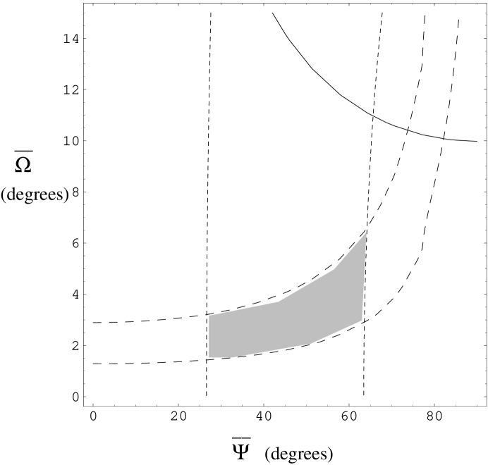
FIG. 1.: The allowed parameter space for $\bar{\Omega}$ and $\bar{\Psi}$. The region below the solid line is allowed by CHOOZ, the region between the almost vertical dotted lines is allowed from the atmospheric data and the region between the dashed lines corresponds to the SMA solution for the solar neutrinos. The shaded region is consistent with all the data.

FIG. 2.: The value of $\tan\beta$ required in MSSM to get a large $\bar{\Psi}$ from a small $\Psi$. The solid (dashed) curve stands for $\Psi=3^{o}~{}(10^{o})$. In each set, the lower (upper) curve denotes $\Delta m^{2}(\Lambda)/m^{2}(\Lambda)=2\cdot 10^{-3}~{}(7\cdot 10^{-3})$ eV² for the $\nu_{2}$-$\nu_{3}$ pair. We have chosen $\Lambda/\mu\sim 10^{10}$.

REFERENCES

- [1] Super-Kamiokande Collaboration: Phys. Rev. Lett. 82, 2644 (1999).
- [2] J. N. Bahcall, P. I. Krastev and A. Yu. Smirnov, Phys. Rev. D58, 096016 (1998); G. L. Fogli, E. Lisi, A. Marrone and G. Scoscia, Phys. Rev. D59, 033001 (1999); M.C. Gonzalez-Garcia, P.C. de Holanda, C. Pena-Garay, J.W.F. Valle, hep-ph/9906469 (to be published in Nucl. Phys. B).
- [3] H. Fritzsch and Z. Xing, hep-ph/9903499 ; F. Vissani, hep-ph/9708483 ; G. K. Leontaris, S. Lola, C. Scheich and J. D. Vergados, Phys. Rev. D53, 6381 (1996) ; B. C. Allanach, hep-ph/9806294 ; V. Barger, S. Pakvasa, T. J. Weiler and K. Whisnant, Phys. Lett. B437, 107 (1998); A. J. Baltz, A. S. Goldhaber and M. Goldhaber, Phys. Rev. Lett. 81, 5730 (1998); R. N. Mohapatra and S. Nussinov, Phys. Lett. B441, 299 (1998) ; Y. Nomura and Y. Yanagida, Phys. Rev. D59, 017303 (1999) ; S. K. Kang and C. S. Kim, Phys. Rev. D59, 091302 (1999) ; G. Altarelli and F. Feruglio, Phys. Lett. B439, 112 (1998) and JHEP 9811, 021 (1998) ; R. Barbieri, L. J. Hall, G. L. Kane and G. G. Ross, hep-ph/9901228 ; A. S. Joshipura and S. Rindani, Phys. Lett. B464, 239 (1999); E. Ma, Phys. Lett. B456, 201 (1999); R. N. Mohapatra, A. Perez Lorenzana and C. Pires, hep-ph/9911395 (To appear in Phys. Lett. B).
- [4] C. Albright, K. S. Babu and S. Barr, hep-ph/9805266; B. Brahmachari and R. N. Mohapatra, Phys. Rev. D58, 15003 (1998); K. S. Babu, J. C. Pati and F. Wilczek, hep-ph/9812538.
- [5] K. R. S. Balaji, A. S. Dighe, R. N. Mohapatra and M. K. Parida, hep-ph/0001310.
- [6] T. K. Kuo and J. Pantaleone, Rev. Mod. Phys. 61, 937 (1989).
- [7] A. De Rujula, M. B. Gavela and P. Hernandez, hep-ph/0001124.
- [8] CHOOZ Collaboration: M. Apollonio et al, Phys. Lett. B420, 397 (1998); hep-ex/9907037.
- [9] K. S. Babu, C. N. Leung and J. Pantaleone, Phys. Lett. B319, 191 (1993); P. H. Chankowski and Z. Pluciennik, Phys. Lett. B316, 312 (1993); M. Tanimoto, Phys. Lett. B360, 41 (1995).
- [10] N. Haba, N. Okamura and M. Sugiura, hep-ph/9810471; N. Haba, Y. Matsui, N. Okamura and M. Sugiura, hep-ph/9908429; J. Ellis and S. Lola, Phys. Lett. B458, 310 (1999) ; J. A. Casas, J. R. Espinosa, A. Ibarra and I. Navarro, hep-ph/9905381.
- [11] SuperKamiokande Collaboration: Phys. Rev. Lett. 81, 1562 (1998).
- [12] K. Scholberg, for the SuperKamiokande Collaboration, hep-ex/9905016; T. Kajita, Invited talk at PASCOS99, December ’99.
- [13] D. White, for the LSND Collaboration, Nucl. Phys. Proc. Suppl. 77, 207 (1999).
- [14] D. Caldwell and R. N. Mohapatra, Phys. Rev. D48, 3259 (1993); J. Peltoniemi and J. W. F. Valle, Nucl. Phys. B406, 409 (1993); S. Bilenky, C. Giunti and W. Grimus, Euro. Phys. J. C1, 247 (1998); Phys. Rev. D57, 1920 (1998); D58, 033001 (1998); E. Ma and P. Roy, Phys. Rev. D52, 4780 (1995).