Higgs Boson Decays to $\tau$-pairs
in the $s$-channel at a Muon Collider

Abstract

We study the observability of the $\tau^{-}\tau^{+}$ decay mode of a Higgs boson produced in the $s$-channel at a muon collider. We find that the spin correlations of the $\tau^{-}\tau^{+}$ in $\tau\to\pi\nu_{\tau},\ \rho\nu_{\tau}$ decays are discriminative between the Higgs boson signal and the Standard Model background. Observation of the predicted distinctive distribution can confirm the spin-0 nature of the Higgs resonance. The relative coupling strength of the Higgs boson to $b$ and $\tau$ can also be experimentally determined.

I Introduction

The Higgs boson is a crucial ingredient for electroweak symmetry breaking in the Standard Model (SM) and in supersymmetric (SUSY) theories. In the minimal supersymmetric standard model (MSSM), the mass of the lightest Higgs boson must be less than about 135 GeV [1], and in a typical weakly coupled SUSY theory $m_{h}$ should be lighter than about 150 GeV [2]. On the experimental side, the non-observation of Higgs signal at the LEP-II experiments has established a lower bound on the SM Higgs boson mass of 106.2 GeV at a 95% Confidence Level (CL) [3] and future searches at LEP-II may eventually be able to explore a SM Higgs boson with a mass up to 110 GeV. If the Fermilab Tevatron can reach an integrated luminosity of $10-30$ fb^-1, then it should be possible to observe a Higgs boson with 5$\sigma$ signal for $m_{h}<130$ GeV and even possibly to 190 GeV with a weaker signal [4]. The CERN Large Hadron Collider (LHC) is believed to be able to cover up to the full $m_{h}$ range of theoretical interest, to about 1000 GeV [5], although it may be challenging to discover a Higgs boson in the “intermediate” mass region 110 GeV $<m_{h}<$ 150 GeV due to the huge SM background to $h\to b\bar{b}$ and the requirement of excellent di-photon mass resolution for the $h\to\gamma\gamma$ signal.

Once a Higgs boson is discovered, it will be of major importance to determine its properties to high precision. It has been pointed out that precision measurements of the Higgs mass, width and the primary decay rates such as $h\to b\bar{b},\ WW^{*}$ and $ZZ^{*}$, can be obtained via the $s$-channel resonant production of a neutral Higgs boson at the first muon collider (FMC) [6]. To determine the Higgs boson couplings and other properties, it is necessary to observe as many decay channels as possible.

A particularly important channel is the $\tau^{-}\tau^{+}$ final state

$$\mu^{-}\mu^{+}\to\tau^{-}\tau^{+}.$$ (1)

In the SM at tree level, this $s$-channel process proceeds in two ways, via $\gamma/Z$ exchange and Higgs boson exchange. The former involves the SM gauge couplings and presents a characteristic $FB$ (forward-backward in the scattering angle) asymmetry and a $LR$ (left-right in beam polarization) asymmetry; the latter is governed by the Higgs boson couplings to $\mu^{-}\mu^{+},\tau^{-}\tau^{+}$ proportional to the fermion masses and is isotropic in phase space due to spin-0 exchange. With the possibility for beam polarizations of a muon collider, the asymmetries were studied in Ref. [7] to improve the Higgs boson signal to background ratio. The unambiguous establishment of the $\tau^{-}\tau^{+}$ signal would allow a determination of the relative coupling strength of the Higgs boson to $b$ and $\tau$ and thus test the usual assumption of $\tau-b$ unification in SUSY GUT theories. The angular distribution would probe the spin property of the Higgs resonance.

In this paper, we propose to make additional use of spin correlations in the final state $\tau^{-}\tau^{+}$ events. We will demonstrate the significant difference of spin correlations between the background events from the spin-1 $\gamma/Z$ exchange and the signal events from the spin-0 Higgs exchange. The correlation is particularly strong for the two-body decay modes for $\tau\to\pi\nu_{\tau},\ \rho\nu_{\tau}$. In Sec. II, we analyze the $\tau^{-}\tau^{+}$ production and decay and present our results. In sec. III, we provide further discussions on the results and draw our conclusion.

II analysis

The $s$-channel Higgs boson (spin-0) exchange populates the $\mu^{-}\mu^{+}$ helicity combinations of left-left ($LL$) and right-right ($RR$). This results in the correlation of $\tau^{-}\tau^{+}$ polarization of $LL$ and $RR$ by angular momentum conservation. In contrast, the SM background channel yields $\tau^{-}\tau^{+}$ polarization combination of left-right ($LR$) and right-left ($RL$). By studying the decay products from the correlated and polarized $\tau^{\pm}$, we can effectively distinguish these two channels and gain information about the spin of the resonance.

A Production cross section for $\mu^{-}\mu^{+}\to\tau^{-}\tau^{+}$

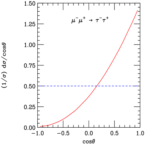
FIG. 1.: Normalized differential cross section for $\mu^{-}\mu^{+}\to\tau^{-}\tau^{+}$. The solid curve is for the SM $\gamma/Z$ exchange and the dashed line is for a scalar $h$ exchange.

The differential cross section for $\mu^{-}\mu^{+}\to\tau^{-}\tau^{+}$ via $s$-channel Higgs ($h$) exchange can be expressed as

$${{d\sigma_{h}(\mu^{-}\mu^{+}\to h\to\tau^{-}\tau^{+})}\over{d\cos\theta}}={1\over 2}{\overline{\sigma}_{h}}\ (1+P_{-}P_{+})$$ (2)

where $\theta$ is the scattering angle between $\mu^{-}$ and $\tau^{-}$, $P_{\mp}$ the percentage longitudinal polarizations of the initial $\mu^{\mp}$ beams, with $P=-1$ purely left-handed, $P=+1$ purely right-handed and $P=0$ unpolarized. ${\overline{\sigma}_{h}}$ is the integrated unpolarized cross section convoluted with the collider energy distribution [6],

$${\overline{\sigma}_{h}}\approx{4\pi\over m^{2}_{h}}\ {B(h\to\mu^{-}\mu^{+})B(h\to\tau^{-}\tau^{+})\over\left[1+{8\over\pi}\left({\sigma_{\sqrt{s}}\over\Gamma_{h}}\right)^{2}\right]^{1/2}}$$ (3)

where $B(h\to\ell^{-}\ell^{+})$ is the Higgs decay branching fraction and $\Gamma_{h}$ is the total width. The Gaussian rms spread in the beam energy $\sqrt{s}$ is given by

$$\sigma_{\sqrt{s}}={R\over\sqrt{2}}{\sqrt{s}},$$ (4)

with $R$ the energy resolution of each beam, anticipated in the range $R\sim 0.05\%-0.005\%$. Note that for a very narrow Higgs boson, like that of the SM for $m_{h}<140$ GeV, the cross section in Eq. (3) is proportional to ${\Gamma_{h}/\sigma_{\sqrt{s}}}$.

The unpolarized cross section for the SM background can be written as

$${d\sigma_{SM}(\mu^{-}\mu^{+}\to\gamma^{*}/Z^{*}\to\tau^{-}\tau^{+})\over{d\cos\theta}}={3\over 8}\sigma_{QED}\ [A(1+\cos^{2}\theta)+B\cos\theta],$$ (5)

where $\sigma_{QED}$ is the QED cross section for $\mu^{-}\mu^{+}\to\gamma^{*}\to\tau^{-}\tau^{+}$ and the coefficients $A$ and $B$ are functions of the c. m. energy and gauge couplings [8]. The interference between the vector current and the axial-vector current leads to a forward-backward asymmetry characterized by

$${A_{FB}}={{\int_{0}^{1}d\cos\theta(d\sigma/d\cos\theta)-\int_{-1}^{0}d\cos\theta(d\sigma/d\cos\theta)}\over{\int_{-1}^{1}d\cos\theta(d\sigma/d\cos\theta)}}={3\over 8}{B\over A}\ .$$ (6)

Furthermore, the chiral neutral current couplings lead to a left-right asymmetry which can be characterized by $A_{LR}$ defined as

$$A_{LR}={{\sigma_{LR\to LR+RL}-\sigma_{RL\to LR+RL}}\over{\sigma_{LR\to LR+RL}+\sigma_{RL\to LR+RL}}}\ .$$ (7)

Again with longitudinal polarizations $P_{\mp}$ for the $\mu^{\mp}$ beams, the differential cross section for the SM background is

$${d\sigma_{SM}\over d\cos\theta}={3\over 8}\sigma_{QED}A[1-P_{+}P_{-}+(P_{+}-P_{-})A_{LR}](1+\cos^{2}\theta+{8\over 3}\cos\theta A^{eff}_{FB}).$$ (8)

Here the effective $FB$ asymmetry factor is

$$A^{eff}_{FB}={{A_{FB}+P_{eff}A_{LR}^{FB}}\over{1+P_{eff}A_{LR}}},$$ (9)

the effective polarization is

$$P_{eff}={{P_{+}-P_{-}}\over{1-P_{+}P_{-}}},$$ (10)

and

$$A_{LR}^{FB}={{\sigma_{LR+RL\to LR}-\sigma_{LR+RL\to RL}}\over{\sigma_{LR+RL\to LR}+\sigma_{LR+RL\to RL}}}\ .$$ (11)

For the case of interest where initial and final state particles are leptons, $A_{LR}=A_{LR}^{FB}$.

From the cross section formulas of Eqs. (2) and (8), the enhancement factor of the signal-to-background ratio ($S/B$) due to the beam polarization effects is

$${S\over B}\sim{1+P_{-}P_{+}\over 1-P_{-}P_{+}+(P_{+}-P_{-})A_{LR}}\ .$$ (12)

The normalized differential cross section for $\mu^{-}\mu^{+}\to\tau^{-}\tau^{+}$ at $\sqrt{s}=m_{h}=120$ GeV is shown in Fig. 1 for both the SM $\gamma/Z$ exchange (solid curve) and a scalar $h$ exchange (dashed line). We see that the SM distribution exhibits a clear forward-backward asymmetry; while the scalar exchange is flat, as expected. Calculation shows that at this c. m. energy, the SM process yields $A_{FB}\sim 0.7$ while $A_{LR}\sim 0.15$. Using the initial polarized beam and the forward-backward asymmetry to improve the precision measurement has been discussed in [7].

B $\tau$ decay and final state spin correlation

$\tau$ decay modes	$\mu\bar{\nu}_{\mu}\nu_{\tau}$	$e\bar{\nu}_{e}\nu_{\tau}$	$\pi\nu_{\tau}$	$\rho\nu_{\tau}$	$a_{1}\nu_{\tau}$
branching fraction $B_{i}\ (\%)$	17.37	17.81	11.08	25.02	18.38

TABLE I.: $\tau$ decay modes and branching fractions from Ref. [9].

As noted previously, the final state polarization configurations of $\tau^{-}\tau^{+}$ from the Higgs signal and the SM background are very different. The $\tau$ decay modes and their branching fractions ($B_{i}$) are listed in Table I. The vector and axial vector resonances $\rho$ and $a_{1}$ subsequently decay into $2\pi$ and $3\pi$ respectively and the vector meson masses can be reconstructed from the final state poins. There is always a charged track to define a kinematical distribution for the decay. In the $\tau$-rest frame, the normalized differential decay rate can be written as

$${1\over\Gamma}{d\Gamma_{i}\over{d\cos\theta}}={B_{i}\over 2}(a_{i}+b_{i}P_{\tau}\cos\theta)$$ (13)

where $\theta$ is the angle between the momentum direction of the charged decay product in the $\tau$-rest frame [10] and the $\tau$-momentum direction, $B_{i}$ is the branching fraction listed in Table I, and $P_{\tau}=\pm 1$ is the $\tau$ helicity. For the two-body decay modes, $a_{i}$ and $b_{i}$ are constant and given by

$$a_{\pi}=b_{\pi}=1,$$ (14)

$$a_{i}=1\quad{\rm and}\quad b_{i}=-{m_{\tau}^{2}-2m_{i}^{2}\over m_{\tau}^{2}+2m_{i}^{2}}\quad{\rm for}\quad i=\rho,\ a_{1}.$$ (15)

For the three-body leptonic decays, the $a_{e,\mu}$ and $b_{e,\mu}$ are not constant for a given three-body kinematical configuration and are obtained by the integration over the energy fraction carried by the invisible neutrinos. One can quantify the event distribution shape by defining a “sensitivity” ratio parameter

$$r_{i}={b_{i}\over a_{i}}.$$ (16)

For the two-body decay modes, the sensitivities are $r_{\pi}=1,\ r_{\rho}=0.45$ and $r_{a_{1}}=0.007$. The $\tau\to a_{1}\nu_{\tau}$ mode is consequently less useful in connection with the $\tau$ polarization study. As to the three-body leptonic modes, although experimentally readily identifiable, the energy smearing from the decay makes it hard to reconstruct the $\tau^{-}\tau^{+}$ final state spin correlation.

FIG. 2.: Double differential distribution for $\mu^{-}\mu^{+}\to h\to\tau^{-}\tau^{+}\to\rho^{-}\nu_{\tau}\rho^{+}\bar{\nu}_{\tau}$. $\sqrt{s}=m_{h}=120$ GeV is assumed. Initial $\mu^{\mp}$ beam polarizations are taken to be $P_{-}=P_{+}=0.25$. The Higgs production cross section is convoluted with Gaussian energy distribution for a resolution $R=0.05\%$.

The differential distribution for the two charged particles ($i,j$) in the final state from $\tau^{-}\tau^{+}$ decays respectively can be expressed as

$${d\sigma\over{d\cos\theta_{i}d\cos\theta_{j}}}\sim\sum_{P_{\tau}=\pm 1}{B_{i}B_{j}\over 4}\ (a_{i}+b_{i}P_{\tau^{-}}\cos\theta_{i})(a_{j}+b_{j}P_{\tau^{+}}\cos\theta_{j}),$$ (17)

where $\cos\theta_{i}\ (\cos\theta_{j})$ is defined in $\tau^{-}\ (\tau^{+})$ rest frame as in Eq. (13). For the Higgs signal channel, $\tau^{-}\tau^{+}$ helicities are correlated as $LL\ (P_{\tau^{-}}=P_{\tau^{+}}=-1)$ and $RR\ (P_{\tau^{-}}=P_{\tau^{+}}=+1)$. This yields the spin-correlated differential cross section

$${d\sigma_{h}\over{d\cos\theta_{i}d\cos\theta_{j}}}=(1+P_{-}P_{+})\sigma_{h}\ {B_{i}B_{j}\over 4}\ [a_{i}a_{j}+b_{i}b_{j}\cos\theta_{i}\cos\theta_{j}],$$ (18)

where the factor $(1+P_{-}P_{+})$ comes from the initial $\mu^{\mp}$ beam polarization; $\sigma_{h}$ is the unpolarized total cross section. We expect that the distribution reaches maximum near $\cos\theta_{i}=\cos\theta_{j}=\pm 1$ and minimum near $\cos\theta_{i}=-\cos\theta_{j}=\pm 1$. How significant the peaks are depends on the sensitivity parameter in Eq. (16). Here we simulate the double differential distribution of Eq. (18) for $\mu^{-}\mu^{+}\to h\to\tau^{-}\tau^{+}\to\rho^{-}\nu_{\tau}\rho^{+}\bar{\nu}_{\tau}$ and the result is shown in Fig. 2. Here we take $\sqrt{s}=m_{h}=120$ GeV for illustration. The Higgs production cross section is convoluted with Gaussian energy distribution [6] for a resolution $R=0.05\%$. We see distinctive peaks in the distribution near $\cos\theta_{\rho^{-}}=\cos\theta_{\rho^{+}}=\pm 1$, as anticipated. In this demonstration, we have taken $\mu^{\mp}$ beam polarizations to be $P_{-}=P_{+}=25\%$, which is considered to be natural with little cost to beam luminosity [11].

FIG. 3.: Double differential distribution for $\mu^{-}\mu^{+}\to\gamma^{*}/Z^{*}\to\tau^{-}\tau^{+}\to\rho^{-}\nu_{\tau}\rho^{+}\bar{\nu}_{\tau}$. $\sqrt{s}=120$ GeV is assumed. Initial $\mu^{\mp}$ beam polarizations are taken to be $P_{-}=P_{+}=0.25$. The SM production cross section is convoluted with Gaussian energy distribution for a resolution $R=0.05\%$.

In contrast, the SM background via $\gamma^{*}/Z^{*}$ produces $\tau^{-}\tau^{+}$ with helicity correlation of $LR\ (P_{\tau^{-}}=-P_{\tau^{+}}=-1)$ and $RL\ (P_{\tau^{-}}=-P_{\tau^{+}}=+1)$. Furthermore, the numbers of the left-handed and right-handed $\tau^{-}$ at a given scattering angle are different because of the left-right asymmetry, so the initial muon beam polarization affects the $\tau^{-}\tau^{+}$ spin correlation non-trivially. Summing over the two polarization combinations in $\tau^{-}\tau^{+}$ decay to particles $i$ and $j$, we have

$${d\sigma_{SM}\over{d\cos\theta_{i}d\cos\theta_{j}}}= (1-P_{-}P_{+})\sigma_{SM}\ (1+P_{eff}A_{LR})\times$$ (20)

$${B_{i}B_{j}\over 4}[(a_{i}a_{j}-b_{i}b_{j}\cos\theta_{i}\cos\theta_{j})+A^{eff}_{LR}(a_{i}b_{j}\cos\theta_{j}-a_{j}b_{i}\cos\theta_{i})].$$

The effective $LR$-asymmetry factor is given by

$$A^{eff}_{LR}\equiv{{\sigma^{eff}_{LR+RL\to LR}-\sigma^{eff}_{LR+RL\to RL}}\over{\sigma^{eff}_{LR+RL\to LR}+\sigma^{eff}_{LR+RL\to RL}}}={{A_{LR}^{FB}+P_{eff}A_{FB}}\over{1+P_{eff}A_{LR}}},$$ (21)

with $\sigma^{eff}$ the cross section including the percentage beam polarization $P_{\pm}$. The final state spin correlation for $\mu^{-}\mu^{+}\to\gamma^{*}/Z^{*}\to\tau^{-}\tau^{+}$ decaying into $\rho^{-}\rho^{+}$ pairs is shown in Fig. 3. The maximum regions near $\cos\theta_{\rho^{-}}=-\cos\theta_{\rho^{+}}=\pm 1$ are clearly visible. Most importantly, the peak regions in Figs. 2 and 3 occur exactly in the opposite positions from the Higgs signal. We also note that the spin correlation from the Higgs signal is symmetric, while that from the background is not. The reason is that the effective $LR$-asymmetry in the background channel changes the relative weight of the two maxima, which becomes transparent from the last term in Eq. (20).

$\sqrt{s}=m_{h}$ (GeV)	$100$	$110$	$120$	$130$
$\sigma_{B}$	55000	19300	12000	8900
$\sigma_{S}\ (R=0.05\%)$	478	380	286	189
$S/B\ (\%)$	0.87	2.0	2.4	2.1
$S/\sqrt{B}\ (1~{}\rm fb^{-1})$	2.0	2.7	2.6	2.0
$\sigma_{S}\ (R=0.01\%)$	2140	1690	1250	806
$S/B\ (\%)$	3.9	8.8	10	9.0
$S/\sqrt{B}\ (1~{}\rm fb^{-1})$	9.1	12	11	8.5
$\sigma_{S}\ (R=0.005\%)$	3750	2970	2170	1350
$S/B\ (\%)$	6.8	15	18	15
$S/\sqrt{B}\ (1~{}\rm fb^{-1})$	16	21	20	14

TABLE II.: Total cross sections (in units of fb) of $\mu^{-}\mu^{+}\to\tau^{-}\tau^{+}$ for the $s$-channel Higgs signal for $\sqrt{s}=m_{h}=100-130$ GeV and the SM background. Also shown are the signal-to-background ratio ($S/B$) and the signal statistical significance ($S/\sqrt{B}$) for an integrated luminosity of 1 $\rm fb^{-1}$. The Higgs channel cross sections are evaluated for three different beam resolutions ($R$). The polarization of the initial $\mu$ beams is taken to be zero.

C Results

The total cross sections of the $s$-channel Higgs signal ($\sigma_{S}$) and the SM background ($\sigma_{B}$) for $\mu^{-}\mu^{+}\to\tau^{-}\tau^{+}$ are listed in Table II with $\sqrt{s}=m_{h}=100-130$ GeV. We show the signal results for three different beam energy resolutions $R=0.05\%,\ 0.01\%$ and $0.005\%$. A better beam energy resolution significantly improves the signal rate for the very narrow Higgs resonance with a width of order of a few MeV, while it has a negligible effect on the background rate. Also shown in the Table are the signal-to-background ratios ($S/B$) and the signal statistical significances ($S/\sqrt{B}$) for an integrated luminosity of 1 $\rm fb^{-1}$. We expect signals that are quite statistically significant. Even if we consider a luminosity of only 0.1 $\rm fb^{-1}$ and include only the clean channels listed in Table I that count for $90\%$ of the branching fraction, the $R=0.005\%$ case still gives a significance better than 3$\sigma$.

As a further refinement in the analyses, we demand the final state $\tau^{-}\tau^{+}$ to be away from the beam hole by $15^{\circ}$, or equivalently

$$|\cos\theta|<0.97.$$ (22)

This reduces the signal rate by about $3\%$ and the background rate by about $5\%$. One could expect to improve the signal observability by imposing more stringent cuts on $\cos\theta$ [7].

$\sqrt{s}=m_{h}$ (GeV)	$100$	$110$	$120$	$130$
$P_{+}=P_{-}=0,\ {\rm no\ cut}$
$\sigma_{B}$	3450	1210	754	559
$\sigma_{S}\ (R=0.05\%)$	29.9	23.8	17.8	11.9
$S/B\ (\%)$	0.87	2.0	2.4	2.1
$\sigma_{S}\ (R=0.01\%)$	134	106	78.5	52.9
$S/B\ (\%)$	3.8	8.8	10	9.4
$\sigma_{S}\ (R=0.005\%)$	235	186	136	84.3
$S/B\ (\%)$	6.8	15	18	15
$P_{+}=P_{-}=0,\ {\rm cut}\ (\ref{cuts})$
$\sigma_{B}$	1630	573	357	265
$\sigma_{S}\ (R=0.05\%)$	15.7	12.5	9.38	6.23
$S/B\ (\%)$	0.96	2.2	2.6	2.4
$\sigma_{S}\ (R=0.01\%)$	70.3	55.8	41.3	26.6
$S/B\ (\%)$	4.3	9.7	12	10
$\sigma_{S}\ (R=0.005\%)$	123	97.6	71.2	44.3
$S/B\ (\%)$	7.6	17	20	17
$P_{+}=P_{-}=0.25,\ {\rm cut}\ (\ref{cuts})$
$\sigma_{B}$	1530	537	335	249
$\sigma_{S}\ (R=0.05\%)$	16.7	13.3	9.97	6.62
$S/B\ (\%)$	1.1	2.5	3.0	2.7
$\sigma_{S}\ (R=0.01\%)$	74.7	59.3	43.9	28.2
$S/B\ (\%)$	4.9	11	13	11
$\sigma_{S}\ (R=0.005\%)$	131	104	75.7	47.1
$S/B\ (\%)$	8.6	19	23	19

TABLE III.: Total cross sections (in units of fb) of $\mu^{-}\mu^{+}\to\tau^{-}\tau^{+}\to\rho^{-}\nu_{\tau}\rho^{+}\bar{\nu}_{\tau}$ for the $s$-channel Higgs signal ($S$) at $\sqrt{s}=m_{h}=100-130$ GeV and the SM background ($B$). The polarization of the initial $\mu$ beams is taken to be 0 and $25\%$ for comparison. The Higgs channel cross sections are evaluated for three different beam resolutions ($R$). The signal-to-background ratios ($S/B$) are also given.

We explore another approach instead to exploit the $\tau^{-}\tau^{+}$ spin correlation. From Figs. 2 and 3, we see that if we focus on the kinematical region $\cos\theta_{i}=\cos\theta_{j}\approx\pm 1$, we can substantially improve the ratio $S/B$. We need to preserve a sufficient signal rate by not taking too tight angular cuts. For illustration, we apply the acceptance cuts on the decay angles in $\tau$ rest frame with

$$\cos \theta_{1}\geq 0,\quad\cos\theta_{2}\geq 0,$$ (23)

$${\rm or}\quad \cos \theta_{1}\leq 0,\quad\cos\theta_{2}\leq 0.$$ (24)

In Table III, we give the results for the $\rho^{-}\nu_{\tau}\rho^{+}\bar{\nu}_{\tau}$ final state from $\tau^{-}\tau^{+}$ decay. Because this mode has the largest branching fraction of about $25\%$, the cross section is larger than for other modes. However, the sensitivity parameter in Eq. (16) for this mode is not maximal, being about 0.45. The surviving signal (background) is $53\%$ ($48\%$) after the acceptance cuts of Eq. (24). The $S/B$ after the cuts does not improve much. The $\pi^{-}\nu_{\tau}\pi^{+}\bar{\nu}_{\tau}$ mode has the maximal sensitivity factor of one, but a rather small cross section due to the low branching fraction. The surviving signal (background) is $63\%$ ($38\%$) after the acceptance cuts, and the $S/B$ is appreciably improved. The results are shown in Table IV.

$\sqrt{s}=m_{h}$(GeV)	$100$	$110$	$120$	$130$
$P_{+}=P_{-}=0,\ {\rm no\ cut}$
$\sigma_{B}$	677	237	148	110
$\sigma_{S}\ (R=0.05\%)$	5.86	4.67	3.50	2.32
$S/B\ (\%)$	0.87	2.0	2.4	2.1
$\sigma_{S}\ (R=0.01\%)$	26.2	20.8	15.4	9.90
$S/B\ (\%)$	3.9	8.8	10	9.0
$\sigma_{S}\ (R=0.005\%)$	46.0	36.4	26.6	16.5
$S/B\ (\%)$	6.8	19	18	15
$P_{+}=P_{-}=0,\ {\rm cut}\ (\ref{cuts})$
$\sigma_{B}$	254	88.9	55.5	41.1
$\sigma_{S}\ (R=0.05\%)$	3.66	2.92	2.19	1.45
$S/B\ (\%)$	1.4	3.3	3.9	3.5
$\sigma_{S}\ (R=0.01\%)$	16.4	13.0	9.62	6.19
$S/B\ (\%)$	6.5	15	17	15
$\sigma_{S}\ (R=0.005\%)$	28.8	22.8	16.6	10.3
$S/B\ (\%)$	11	26	30	25
$P_{+}=P_{-}=0.25,\ {\rm cut}\ (\ref{cuts})$
$\sigma_{B}$	238	83.4	52.0	38.6
$\sigma_{S}\ (R=0.05\%)$	3.89	3.10	2.32	1.54
$S/B\ (\%)$	1.6	3.7	4.5	4.0
$\sigma_{S}\ (R=0.01\%)$	17.4	13.8	10.2	6.58
$S/B\ (\%)$	7.3	17	20	17
$\sigma_{S}\ (R=0.005\%)$	30.6	24.2	17.7	11.0
$S/B\ (\%)$	13	29	34	29

TABLE IV.: Total cross sections (in units of fb) of $\mu^{-}\mu^{+}\to\tau^{-}\tau^{+}\to\pi^{-}\nu_{\tau}\pi^{+}\bar{\nu}_{\tau}$ for the $s$-channel Higgs signal at $\sqrt{s}=m_{h}=100-130$ GeV and the SM background. The polarization of the initial $\mu$ beams is taken to be 0 and $25\%$ for comparison. The Higgs channel cross sections are evaluated for three different beam resolutions ($R$). The signal-to-background ratios ($S/B$) are also given.

A $25\%$ polarization of both beams only slightly improves the signals and decreases the backgrounds, as implied by Eq. (12). Higher beam polarization could help improve $S/B$, but perhaps at a significant cost to the luminosity [11].

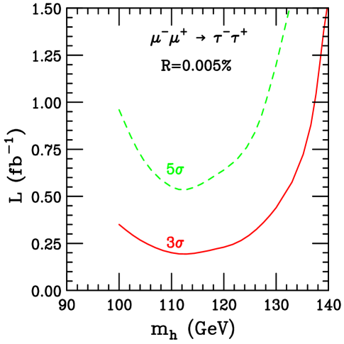
FIG. 4.: Integrated luminosity (in $\rm fb^{-1}$) needed for observing the two-body decay channels $\tau\to\rho\nu_{\tau}$ and $\tau\to\pi\nu_{\tau}$ at $3\sigma$ (solid) and $5\sigma$ (dashed) significance. Beam energy resolution $R=0.005\%$ and a $25\%$ polarization are assumed.

We next estimate the luminosity needed for signal observation of a given statistical significance. The results are shown in Fig. 4. The integrated luminosity ($L$ in $\rm fb^{-1}$) needed for observing the characteristic two-body decay channels $\tau\to\rho\nu_{\tau}$ and $\tau\to\pi\nu_{\tau}$ at $3\sigma$ (solid) and $5\sigma$ (dashed) significance is calculated for both signal and SM background with $\sqrt{s}=m_{h}$. Beam energy resolution $R=0.005\%$ and a $25\%$ $\mu^{\pm}$ beam polarization are assumed.

Based on Tables III and IV, we estimate the statistical error on the cross section measurement. If we take the statistical error to be given by

$$\epsilon={\sqrt{S+B}\over S}={1\over\sqrt{L}}\ {\sqrt{\sigma_{S}+\sigma_{B}}\over\sigma_{S}},$$ (25)

summing over both $\rho\nu_{\tau}$ and $\pi\nu_{\tau}$ channels for $R=0.005\%$, a $25\%$ beam polarization with 1 $\rm fb^{-1}$ luminosity, we obtain

$$\begin{array}[]{lcccc}\sqrt{s}=m_{h}\ (\rm GeV)&100&110&120&130\\ \epsilon\ (\%)&27&21&23&32\end{array}$$ (26)

The uncertainties on the cross section measurements determine the extent to which the $h\tau^{-}\tau^{+}$ coupling can be measured.

III Discussion and conclusion

If we only consider the $\pi\nu_{\tau}$ and $\rho\nu_{\tau}$ channels that best preserve the $\tau^{-}\tau^{+}$ spin correlation, the effective branching fraction is only $36\%$ and we may be limited by statistics. However, the distinctively different double differential distributions of the signal and the SM backgrounds may provide definitive information for determining the spin of the resonant Higgs particle. When analyzing the data sample, one may consider a sophisticated fitting to the superposition of the signal and background distributions.

The characteristic angular distributions of polarized $\tau$ decays are only simply manifest in the $\tau$ rest frame. It is thus desirable to infer the $\tau^{\pm}$ momenta in order to boost the final state particles ($\rho,\ \pi,\ \ell^{\pm}$ etc.) to the parent $\tau$ rest frame. Because of the excellent energy calibration of a muon collider, it is a good approximation to assume each $\tau$ to have an energy of $\sqrt{s}/2$. However, it may be experimentally challenging to determine the $\tau$ momentum direction. One of the possible methods is to locate the secondary vertices for $\tau$ decays. The impact parameter for $\tau$ decays is $\ell/\gamma\approx\beta c\tau_{\tau}\approx 87\ \mu$m. This should be sufficiently large to be resolved by vertex detectors.

It is important to note that it is not necessary to fully reconstruct the $\tau$ momenta for the clean two-body channels. This is because the polar angles ($\theta_{1},\theta_{2}$) in the $\tau$ rest frame can be uniquely determined by the charged particle energy [10]. If the lab-frame energy for $\rho,\pi$ is $E_{i}$, then the relation to the polar angle is

$$\cos\theta_{i}={2z_{i}-1-a^{2}\over\beta(1-a^{2})},$$ (27)

where the energy fraction $z_{i}=2E_{i}/\sqrt{s}$, $a=m_{i}/m_{\tau}$ and $\beta$ is the velocity of the decay product. Due to the unique linear relation between $\cos\theta_{i}$ and $z_{i}$, two dimensional correlation plots for $z_{i}-z_{j}$ can be obtained in a similar fashion as Figs. 2 and 3.

The $s$-channel Higgs signal at the FMC could provide a precision measurement for the Higgs total width [6], and thus lead to the determination of the coupling strength parameter $\tan\beta$ in SUSY theories. The observation of the $h\to\tau^{-}\tau^{+}$ channel in addition to the channel $h\to b\bar{b}$ is very important: The relative strength of the Higgs couplings to $b$ and to $\tau$ could be an indicator to the underlying physics, such as the possibly large non-universal radiative effects in MSSM [12] from the chargino and gluino loops, and radiatively generated Yukawa couplings [13]. We expect that the measurement of the coupling ratio is robust, and only statistically limited in the $\tau^{-}\tau^{+}$ mode. If a high degree of transverse polarization of the beams is achievable, one could consider the possibility to determine the CP properties of the Higgs boson coupling [6, 14] by making use of the $\tau^{-}\tau^{+}$ mode.

In summary, we have demonstrated the feasibility of observing the resonant channel $h\to\tau^{-}\tau^{+}$ at a muon collider. For a narrow resonance like the SM Higgs boson, a good beam energy resolution is crucial for a clear signal. On the other hand, a moderate beam polarization would not help much for the signal identification. The integrated luminosity needed for a signal observation is presented in Fig. 4. Estimated statistical errors for the $\mu^{-}\mu^{+}\to h\to\tau^{-}\tau^{+}$ cross section measurement are given in Eq. (26). We emphasized the importance of final state spin correlation to purify the signal of a scalar resonance and to confirm the nature of its spin. It is also important to carefully study the $\tau^{-}\tau^{+}$ channel of a supersymmetric Higgs boson which would allow a determination of the relative coupling strength of the Higgs to $b$ and $\tau$.

Acknowledgments: We thank Dieter Zeppenfeld for discussions on the $\tau$ polarization. This work was supported in part by a DOE grant No. DE-FG02-95ER40896 and in part by the Wisconsin Alumni Research Foundation.

REFERENCES

- [1] H. E. Haber and R. Hempfling, Phys. Rev. Lett. 66, 1815 (1991); R. Hempfling and A. H. Hoang, Phys. Lett. B331, 99 (1994); M. Carena, J.R. Espinosa, M. Quiros and C.E.M. Wagner, Phys. Lett. B355, 209 (1995); H. E. Haber, R. Hempfling and A. H. Hoang, Z. Phys. C75, 539 (1997); S. Heinemeyer, W. Hollik and G. Weiglein, Phys. Rev. D58, 091701 (1998); R.-J. Zhang, Phys. Lett. B447, 89 (1999); J. R. Espinosa and R.-J. Zhang, hep-ph/9912236; M. Carena, H. E. Haber, S. Heinemeyer, W. Hollik, C.E.M. Wagner and G. Weiglein, hep-ph/0001002.
- [2] G. L. Kane, C. Kolda and J. D. Wells, Phys. Rev. Lett. 70, 2686 (1993).
- [3] P. McNamara, talk presented at the LEPC meeting, September (1999).
- [4] A. Stange, W. Marciano and S. Willenbrock, Phys. Rev. D 49, 1354 (1994); Phys. Rev. D50, 4491 (1994); T. Han and R.-J. Zhang, Phys. Rev. Lett. 82, 25 (1999); T. Han, A. Turcot and R.-J. Zhang, Phys. Rev. D59, 093001 (1999); Higgs working group report for Physics at Tevatron Run II Workshop, http://fnth37.fnal.gov/higgs.html.
- [5] CMS Collaboration, Technical Proposal, CERN/LHCC/94–38 (1994); ATLAS Collaboration, Technical Proposal, CERN/LHCC/94–43 (1994); M. Spira, Fortsch. Phys. 46, 203 (1998).
- [6] V. Barger, M. S. Berger, J. F. Gunion and T. Han, Phys. Rev. Lett. 75, 1462 (1995); Phys. Rep. 286, 1 (1997).
- [7] B. Kamal, W.J. Marciano and Z. Parsa, hep-ph/9712270.
- [8] T. P. Cheng and L. F. Li, Gauge theory of elementary particle physics, Oxford University Press, 1984.
- [9] Particle Data Group, Eur. Phys. J. C3, 1 (1998).
- [10] B. K. Bullock, K. Hagiwara and A. D. Martin, Nucl. Phys. B395, 499 (1993).
- [11] C.M. Ankenbrandt et al., the muon collider collaboration, Phys. Rev. ST Accel. Beams 2, 081001 (1999).
- [12] M. Carena, S. Mrenna and C. Wanger, Phys. Rev. D60, 075010 (1999).
- [13] F. Borzumati, G. Farrar, N. Polonsky and S. Thomas, Nucl. Phys. B555, 53 (1999).
- [14] B. Grzadkowski and J. Gunion, Phys. Lett. B350, 218 (1995); D. Atwood and A. Soni, Phys. Rev. D52, 6271 (1995); D. Atwood, L. Reina and A. Soni, Phys. Rev. Lett. 75, 3800 (1995).