SLAC-PUB-8351 February, 2000

Theoretical Summary Lecture for EPS HEP99

Michael E. Peskin

Stanford Linear Accelerator Center
Stanford University, Stanford, California 94309 USA

ABSTRACT

This is the proceedings article for the concluding lecture of the 1999 High Energy Physics Conference of the European Physical Society. In this article, I review a number of topics that were highlighted at the meeting and have more general importance in high energy physics. The major topics discussed are (1) precision electroweak physics, (2) CP violation, (3) new directions in QCD, (4) supersymmetry spectroscopy, and (5) the experimental physics of extra dimensions.

invited lecture presented at the

International Europhysics Conference on High-Energy Physics

July 15-21, 1999, Tampere, Finland

1 Introduction

In this theoretical summary lecture at the High Energy Physics 99 conference of the European Physical Society, I am charged to review some of the new conceptual developments presented at this conference. At the same time, I would like to review more generally the progress of high-energy physics over the past year, and to highlight areas in which our basic understanding has been affected by the new developments. There is no space here for a status report on the whole field. But I would like to give extended discussion to five areas that I think have special importance this year. These are (1) precision electroweak physics, which celebrates its tenth anniversary this summer; (2) CP violation, which entered a new era this summer with the inauguration of the SLAC and KEK B-factories; (3) QCD, which now branches into new lines of investigation; and two rapidly developing topics from physics beyond the Standard Model, (4) supersymmetry spectroscopy and (5) the experimental study of extra dimensions. A sixth important topic, that of neutrino masses and mixing, is covered in the experimental summary talk of Lorenzo Foa [1]. The location of the conference in Finland makes it appropriate to end the lecture with a Lutheran sermon.

2 Precision Electroweak Physics

This summer marks the tenth anniversary of a watershed in high-energy physics that took place in the summer and fall of 1989. In that year, the UA2 and CDF experiments announced the first truly precision measurements of the $W$ boson mass. These experiments also pushed the mass of the top quark above 60 GeV, thus insuring that radiative corrections due to the top quark would play an important role in the interpretation of weak interaction measurements. SLC and LEP began their high-statistics study of $Z^{0}$ resonance in $e^{+}e^{-}$ annihilation. The data from these machines rapidly produced a $Z^{0}$ mass accurate to four significant figures, limited the number of light neutrinos to 3, and began the program of precisely testing the weak-interaction couplings. In the spring of 1989, it was permissible to believe that the $W$ and $Z$ bosons were composite and that the gauge symmetry of the weak interactions was merely a low-energy approximation. Today, because of the experimental program set in motion that year, this is no longer an option.

It is interesting to contrast our knowledge of the weak interaction parameters in 1989 with our knowledge today. In Figure 1, I show the summary of the constraints on the weak interaction mixing angle $\sin^{2}\theta_{w}$ that were presented by Altarelli at the 1989 Lepton-Photon conference [2]. The vertical axis shows $\sin^{2}\theta_{w}$ in Sirlin’s definition [3]

$$\sin^{2}\theta_{w}\bigr{|}_{{\mbox{\scriptsize Sirlin}}}=1-{m_{W}^{2}\over m_{Z}^{2}}\ .$$ (1)

The horizontal axis shows the top quark mass, which enters the comparison of weak interaction processes through ${\cal O}(\alpha)$ vacuum polarization diagrams. The constraints shown were all new: the Ellis-Fogli fit to deep-inelastic neutrino and electron scattering [4], the UA2 and CDF measurements of $m_{W}/m_{Z}$ [5, 6], and the SLC measurement of the $Z^{0}$ mass [7]. Contrast the precision of this figure, remarkable at the time, with the small trace labeled ‘1999’. This dot represents our current knowledge of $m_{t}$ and $\sin^{2}\theta_{w}$.

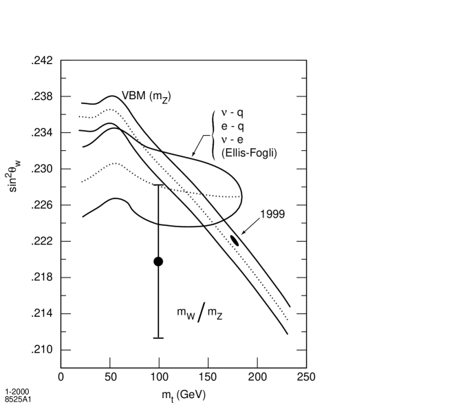
Figure 1: Constraints on $\sin^{2}\theta_{w}$ as a function of the top quark mass, shown by Altarelli at the 1989 Lepton-Photon conference [2]. The small dot marked 1999 shows our current knowledge.

Within a month after Altarelli showed this figure, the LEP collider began its high-statistics study of the $Z^{0}$ resonance. The precision of these experiments, and their remarkable agreement with the Standard Model predictions, has led to a major change in the way that we think about the weak interactions. Today, we regard $m_{Z}$ as a fundamental constant of Nature, determined to precision of five significant figures and thus standing on a par with $\alpha$ and $G_{F}$. The precise values of these three parameters fix the tree-level predictions of the Standard Model. Experiments can then focus on possible small deviations from these predictions, which might be due to the radiative corrections of the Standard Model, or to new physics.

There are several schemes for presenting relatively model-independent constraints on weak interaction radiative corrections. My favorite is to parametrize the $W$ and $Z$ boson vacuum polarization diagrams in terms of two parameters $S$ and $T$, scaled so that an effect of order 1 in these parameters corresponds to a correction of order $\alpha$ in the electroweak observables [8]. (Other similar parameters sets are defined in [9, 10].) The parameter $S$ is weak-isospin conserving and measures the overall size of a new physics sector; the parameter $T$ measures the extent of its weak-isospin violation. The zero point of $S$ and $T$ is fixed by convention; for my discussion here, I will fix it to correspond to the minimal Standard Model with a top quark mass of 175 GeV and a Higgs boson mass of 100 GeV.

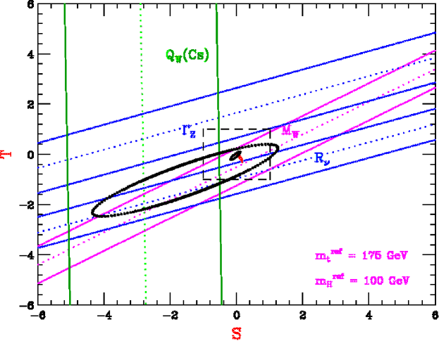
Figure 2: Fits of the corpus of precision electroweak data to the parameters $S$ and $T$, for the data available in the summer of 1989 and the summer of 1999 [11].

In Figure 2, I present the $S$, $T$ fit to the corpus of precision electroweak data from the summer of 1989 and from the summer of 1999, both prepared by Morris Swartz [11]. The bottom figure fits into the small dashed rectangle in the top figure. The current best values are

$$S=-0.04\pm 0.10\ ,\qquad T=-0.06\pm 0.11\ .$$ (2)

What have we learned from this dramatic improvement in our experimental knowledge? I extract three morals:

First, we have learned that the predictions of the minimal Standard Model are amazingly successful! I remind you that the agreement of predictions to better than order-1 on the $S,T$ plot requires radiative corrections, and that the experimental success thus tests the Standard Model at the loop level. This aspect is discussed in more detail in [12].

This level of agreement causes deep difficulty for many schemes of physics beyond the Standard Model. Certain models of new physics have the property that they ‘decouple’ when the scale of new physics becomes large. In brief, this means that new particles of mass $M$ produce corrections to $S$ and $T$ that are of order

$$S\ ,\ T\sim{1\over 4\pi}{m_{Z}^{2}\over M^{2}}\$$ (3)

for $M\gg m_{Z}$. The precision electroweak results imply that, generically, any model of new physics that does not naturally decouple in this way is excluded. This is a severe setback for technicolor models, models with a fourth generation of quarks and leptons, and models in which quarks and leptons are composite. Models with decoupling are typically also models in which the Higgs boson is a fundamental weakly-coupled scalar particle, so the precision electroweak results support this hypothesis.

There are still some notable discrepancies in the picture. In his review at HEP99, Mnich presented a combined value of the $Z$ polarization asymmetry of $b$ quarks [13],

$$A_{b}=0.893\pm 0.016\ \qquad(SM:\ 0.935)\ .$$ (4)

On the other hand, the value of the $b$ fraction of hadronic $Z$ decays has now settled down to

$$R_{b}=0.21642\pm 0.00073\ ,$$ (5)

which agrees with the standard model to 0.3% accuracy. For comparison, technicolor models typically predict a 3% discrepancy [14]. A theorist who wanted to pursue this matter could construct a model with a large deviation in $A_{b}$ and no deviation in $R_{b}$, but essentially all models constructed in advance of the data predicted the opposite pattern.

Further improvements in the precision of the comparison of electroweak data to the Standard Model will require a more precise determination of the renormalization of $\alpha$ from $Q^{2}=0$ to $Q^{2}=m_{Z}^{2}$. This requires a precise knowledge of the total cross section for $e^{+}e^{-}$ annihilation to hadrons through this energy range. We are fortunate that the Beijing Electron Synchrotron has made this measurement a focus of its experimental program and expects to dramatically improve our knowledge of the cross section in the charm threshold region [15].

Second, we have determined the parameters of the Standard Model to remarkable precision. In particular, we now have accurate values for the fundamental Standard Model coupling constants. In terms of $\overline{M\kern-2.0ptS}$ couplings at the scale $m_{Z}$,

$$\alpha^{\prime} = 1/98.42\pm 0.27$$

$$\alpha_{w} = 1/29.60\pm 0.08$$

$$\alpha_{s} = 1/8.40\pm 0.14\ .$$ (6)

At the same time, the precision electroweak data constraints give us information on the mass of the Higgs boson. In a fit to the minimal Standard Model, one now finds [13]

$$m_{H}<245\ \mbox{GeV}\ \qquad\mbox{(95\%\ conf.)}$$ (7)

These results generalize to models with multiple Higgs bosons. Assume, for example, that there are several Higgs bosons $\phi_{i}$ with vacuum expectation values $v_{i}$, and set

$$v=246\ \mbox{GeV}\ .$$ (8)

Then there is a sum rule $\sum_{i}v_{i}^{2}=v^{2}$ [16], and the precision electroweak data adds the information

$$\sum_{i}\left({v_{i}^{2}\over v^{2}}\right)\log{m_{i}\over\mbox{(}245GeV)}<0\ .$$ (9)

In principle, new interactions at high energy can contribute to the right-hand side of (9); however, in the simplest models, these contributions are negative (corresponding to positive contributions to $S$) [8, 17].

Both of the new pieces of information are encouraging for supersymmetry. The precisely known values of the couplings are consistent with a grand unification of couplings if the renormalization group equations of supersymmetry are used in the comparison [18]. Supersymmetric grand unified theories require a Higgs boson below 180 GeV[19, 20, 21]. A useful reference value is the prediction of the minimal supersymmetric generalization of the Standard Model (MSSM), for large superparticle masses and reasonably large $\tan\beta$, $m_{h}\sim 120$ GeV. This should be compared to the new direct search limit on the Higgs boson mass announced at HEP99 [22]

$$m_{h}>95.2\ \mbox{GeV}\ \qquad\mbox{(95\%\ conf.)}\ .$$ (10)

I am still hoping that the Higgs boson will be found at LEP before its time runs out. If not, there is a new entrant into the race to discover the Higgs boson, the Run II Tevatron experiments. A new analysis of Tevatron capabilities takes account of many possible improvements from earlier studies [23]. The Higgs is searched for in the decay mode $h^{0}\to b\overline{b}$ in the reaction $p\overline{p}\to Wh$, with a leptonic decay of the $W$, and $p\overline{p}\to Zh$, with a $\nu\overline{\nu}$ decay of the $Z$. The expected improvements in vertex identification and $b\overline{b}$ mass resolution are included, and the new ability to trigger on displayed vertices plays an important role. The expected sensitivity of the Tevatron experiments is shown in Figure 3. If the Tevatron can accumulate 20 fb^-1 of integrated luminosity, it should be able to find the Higgs boson in the whole region expected in the MSSM, and in most of the region expected for any model with a weakly-coupled Higgs boson.

Figure 3: Expected capability of the Run II Tevatron experiments to observe the minimal Standard Model Higgs boson, at various levels of integrated luminosity [23]. The lower curve shows a preliminary improved analysis based on neural network techniques.

Third, we have acquired a tactile appreciation for the Standard Model couplings to quarks and leptons. The beautiful experiments at the $Z^{0}$ resonance do not simply give the $Z^{0}$ couplings as outputs of a fit; they show directly how the Standard Model works. From the many remarkable plots that have come out of the LEP and SLC program, I show three of my favorites in Figure 4. The upper left shows the ALEPH determination of the $\tau$ polarization at the $Z^{0}$, in which three decay modes, each with its own characteristic physics, show a 14% excess of $\tau_{L}$ over $\tau_{R}$. The upper right shows the profound effect of electron beam polarization on the $b$ angular distribution, characteristic of the almost complete dominance of $b_{L}$ in $Z^{0}$ decays, as observed by the SLD experiment. The lower left shows the OPAL determination of the resonance line-shape for $Z^{0}$ decays to hadrons. The remarkable agreement shown reflects our understanding of all three of the fundamental interactions, weak, through the gross form and precision radiative corrections, strong, through the order $\alpha_{s}$ correction to the decay width to quarks, and electromagnetic, through the distortion of the line-shape by initial-state radiation. In the lower right, I add a new figure shown for the first time at HEP99, the measurement of the $W$ boson production and decay angular distributions by L3 [27]. This shows the forward peak in the production angle expected from neutrino exchange, and the correct proportion of events with central values of the decay angle, characteristic of longitudinal $W$ polarization. All four plots speak directly to the basic underlying physics. It is no longer a tenable position that the Standard Model is a ‘social construct’; we see its reality before our eyes.

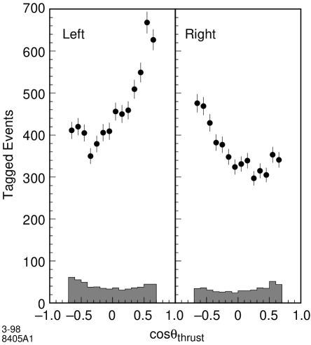
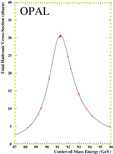
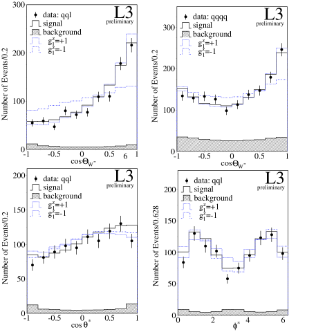
Figure 4: Four figures which display how the Standard Model works at the $Z^{0}$ resonance and at higher energy. See the text for more details.

3 CP violation

Just as this year marks the completion of an era in electroweak physics, it marks the beginning of an era in the study of CP violation. We have seen one of the major questions about CP violation finally answered, and we have seen the first results from new facilities that will dramatically reshape our experimental knowledge.

To put both developments in perspective, I will begin my discussion with a capsule history of CP violation. The phenomenon was discovered in 1964, in the classic experiment of Christensen, Cronin, Fitch, and Turlay [28]. Almost immediately thereafter, Wolfenstein asked a crucial question [29]: Is CP violation a part of the weak interactions, or is it due to a new interaction at very small distances? Over the years, many models have been proposed in which CP violation arises from weak-interaction couplings of particles with masses of the order of $m_{W}$; the Kobayashi-Maskawa model [30], in which CP violation is due to quark mixing, the Weinberg model [31], in which CP violation is due to Higgs boson mixing, and other models in which CP violation comes from phases in the mixing of more exotic species. Behind all of these, though, lurked the possibility of a ‘superweak’ origin for CP violation, in which CP violation arose from a new hard coupling which affected only the $K^{0}$–$\overline{K}{}^{0}$ mixing.

In 1979, Gilman and Wise proposed a crucial test of the weak-interaction origin of CP violation [32]. They showed that such theories typically predict a small but nonzero influence of CP violation on the $K^{0}$ decay amplitudes through the parameter $\epsilon^{\prime}$. In 1988, the CERN NA31 experiment found a nonzero value for $\epsilon^{\prime}$ [33], but this result was not confirmed by the competing experiment E731 at Fermilab [34]. Finally, this year, the new high precision experiments NA48 and KTeV agree that $\epsilon^{\prime}$ is nonzero and find quite similar values [35, 36]. The new world average presented at HEP99 is [37]

$$\epsilon^{\prime}/\epsilon=(21.2\pm 4.6)\times 10^{-4}\ .$$ (11)

The nonzero result in (11) rules out a superweak origin of CP violation. The specific value is too small to be compatible with the original Weinberg model. It is an interesting question whether the value can be compatible with the Kobayashi-Maskawa model or whether it requires new particles with CP violating couplings. This topic was discussed at length at HEP99 [37], and I would like to give my impression of the current situation.

Though the complete formula for $\epsilon^{\prime}/\epsilon$ in the Standard Model is very complicated, one can argue about the uncertainties in $\epsilon^{\prime}/\epsilon$ by using the simplified approximate relation [38]

$$\epsilon^{\prime}/\epsilon = 10^{-4}$$ (12)

$$\hskip-42.67912pt\cdot\left[16B_{6}^{(1/2)}-8B_{8}^{(3/2)}\bigl{(}{m_{t}\over 165}\bigr{)}^{2.5}\right]\biggl{(}{110\over m_{s}}\biggr{)}^{2}\ ,$$

where $m_{t}$ is the $\overline{M\kern-2.0ptS}$ top quark mass evaluated at $m_{t}$, $m_{s}$ is the $\overline{M\kern-2.0ptS}$ strange quark mass evaluated at 2 GeV, and $B_{6}{}^{(1/2)}$ and $B_{8}{}^{(3/2)}$ are conventionally defined factors giving the matrix elements of penguin operators arising from the strangeness-changing weak interaction. The convention for the $B$ coefficients factors out the dependence on the strange quark mass, and one should keep in mind that it is the combination $B/m_{s}^{2}$ which corresponds to a physical matrix element. These matrix elements must be determined by a nonperturbative technique, for example, lattice QCD simulation. The first term in (12) is due to the strong-interaction penguin diagram, the second to the electroweak penguin (as in Figure 5). The strong cancellation between these two effects for large top quark mass is the reason that the observed value of $\epsilon^{\prime}/\epsilon$ is much smaller than the original prediction of Gilman and Wise [39]. The cancellation also amplifies the considerable uncertainties in the operator matrix elements.

Figure 5: Diagrams contributing to $\epsilon^{\prime}/\epsilon$ in $K^{0}$ decays: (a) strong penguin, (b) electroweak penguin.

New estimates of the parameter $B_{8}{}^{(3/2)}$ were reported at HEP99:

$$B_{8}^{(3/2)}\cdot\biggl{(}{110\over m_{s}}\biggr{)}^{2}=\cases{0.91\pm 0.16&\cite[cite]{[\@@bibref{}{Donoghue}{}{}]}\cr 0.86\pm 0.07&\cite[cite]{[\@@bibref{}{Soni}{}{}]}\cr}\ .$$ (13)

Both estimates are given in the chiral limit $m_{s}\to 0$. (For the true value of $m_{s}$, one should multiply these estimates by 1.3.) The first of these estimates is based on perturbative QCD analysis of spectral-function sum rules, the second is derived from a lattice QCD calculation using the new technique of domain-wall chiral fermions [42, 43, 44]. From the agreement, it seems that this part of the problem is now fairly well understood. Unfortunately, the situation for $B_{6}{}^{(1/2)}$ is much worse. This matrix element vanishes in the chiral limit and in the $SU(3)$ limit, making the usual techniques for both lattice gauge theory and QCD estimates awkward to apply. For perturbative QCD estimates, $B_{6}{}^{(1/2)}$ depends on the scalar and pseudoscalar spectral functions, which are poorly known. The operator which is responsible for the $\Delta I=\frac{1}{2}$ rule enhancement of the $K^{0}\to\pi\pi$ matrix element has similar problems, and, indeed, to this day no lattice gauge theory calculation has been able to compute the $\Delta I=\frac{1}{2}$ enhancement accurately. Thus, the value of $B_{6}{}^{(1/2)}$ is not known, and this uncertainty can easily allow one to reconcile the prediction (12) with the observed value (11).

We have now reached the situation in which we know that CP violation arises from weak-interaction couplings, but we do not have a sufficiently good theoretical understanding of the measured observables to know whether CP violation is accounted for by the Kobayashi-Maskawa model or whether new particles with CP violating couplings are required. Fortunately, we are entering a new era in which the SLAC, KEK, and Cornell $e^{+}e^{-}$ B-factories, the HERA-B experiment, and measurements of $B$ decay at high-luminosity hadron colliders will provide measurements of new CP violation observables which can be interpreted with very small theoretical uncertainty. This new era offers us a remarkable opportunity either to put the conventional picture of CP violation on a firm footing or to overturn it and discover signal of new physics. In order to do this, however, we must change our view of what the important CP violation observables are and how we should compare them.

An example of the CP violation observables of the new era is the time-dependent asymmetry ${\cal A}$ in an exclusive $B$ decay, an observable first discussed by Carter and Sanda [45]. For example,

$$\Gamma(\overline{B}^{0}\ \mbox{or}\ B^{0}\to J/\psi K^{0}_{S})\sim e^{-\Gamma t}\left[1\pm{\cal A}\sin\Delta m_{d}t\right]\ .$$ (14)

In this equation, $\Delta m_{d}$ is the $B^{0}_{L}$–$B^{0}_{S}$ mass difference, and the sign $\pm$ refers to the two possible initial states. The parameter ${\cal A}$ is manifestly CP violating and can be extracted with essentially no uncertainty from our knowledge of hadronic matrix elements. In the Kobayashi-Maskawa model, ${\cal A}=\sin 2\beta$, where $\beta$ is simply related to the phase in the Cabibbo-Kobayashi-Maskawa (CKM) mixing matrix. In models with new CP violating couplings, ${\cal A}$ can obtain additional large contributions from these sources.

At HEP99, we had a first taste of the new era of CP violation with the report of the first significant measurement the CP asymmetry in $B^{0}\to J/\psi K^{0}$ by the CDF collaboration [46]. The experiment observed the $J/\psi$ in its decay to $\ell^{+}\ell^{-}$ and the $K^{0}_{S}$ in its decay to $\pi^{+}\pi^{-}$. The initial flavor of the $B^{0}$ was determined either by the lepton charge or jet charge on the opposite side of the event, or by the charge of a pion accompanying the $B^{0}$ in the same jet. The figure of merit for such flavor tags, giving the fraction of the event sample that corresponds to the effective number of perfectly tagged $B^{0}$’s, is

$$\epsilon D^{2}\ ,$$ (15)

where $\epsilon$ is the efficiency of the tag and $D$ is the dilution, the difference between the probability of a correct tag and the probability of a wrong tag. (In the next decade, high-energy physicists will mutter ‘$\epsilon D^{2}$’ as often as, in last one, they were heard to mutter ‘$\sin^{2}\theta_{w}$’.) For the CDF measurement, the $\epsilon D^{2}$ for each of the three tagging methods is about 2%, so that the sample of 400 events corresponds effectively to 25 tagged $B^{0}$ decays. From this, one finds

$${\cal A}=0.79^{+0.41}_{-0.44}\ ,$$ (16)

roughly a $2\sigma$ determination that ${\cal A}>0$. I show the data binned as a function of $t$ in Figure 6 and leave it to you to judge the quality of the evidence.

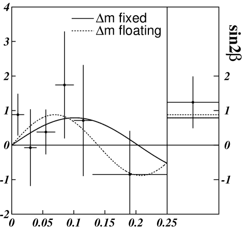
Figure 6: Time-dependent asymmetry in $\overline{B}^{0},B^{0}\to J/\psi K^{0}_{S}$, as measured by the CDF collaboration [46].

Within a year or so, we should have the first accurate measurements of these new CP observables, and we will need a framework to use in comparing them. A useful pictorial device is the ‘unitarity triangle’ [47, 48], the triangle in the complex plane which reflects the unitarity relation of CKM matrix elements

$$V_{ub}V_{ud}^{*}+V_{cb}V_{cd}^{*}+V_{tb}V_{td}^{*}=0\ ,$$ (17)

Using the approximations $V_{ud}\approx V_{tb}\approx 1$, $V_{cd}\approx\sin\theta_{C}$, we find the relation shown in Figure 7. The internal angles of this triangle are referred to as $\alpha$, $\beta$, $\gamma$, except in the Far East, where the notation $\phi_{2}$, $\phi_{1}$, $\phi_{3}$ is used.

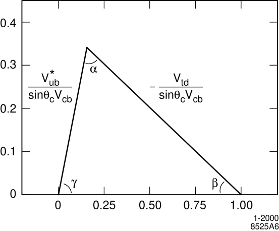
Figure 7: The unitarity triangle.

It is often said that the goal of the new CP violation measurements is to ‘check whether the unitarity triangle closes’. I would like to substitute for this a more precise idea.

Since CP violating phases can be redefined by convention, CP violation observables typically involve phase differences between two different amplitudes. Usually, these are $B$ or $K$ mixing amplitudes or other loop diagrams on one hand, and weak decay amplitudes on the other hand. I will assume that the phases of the decay amplitudes come only from the CKM matrix elements. This is correct unless the decay amplitudes also receive corrections from the tree-level exchange of light exotic particles such as charged Higgs bosons. On the other hand, a loop diagram which contribute to mixing can receive corrections from any new particles with masses in the range up to 1 TeV, and the couplings of these particles can bring new contributions to its phase. If we try to determine the unitarity triangle from a set of processes which all involve the same loop diagram, it is possible to get a consistently determined triangle which does not coincide with the true unitarity triangle of the CKM matrix. The way to test models of CP violation, then, is to compare the unitarity triangles determined from different classes of CP observables. This point of view, set out in the original work of Nir and Silverman [49], has been emphasized more recently by Cohen, Kaplan, Lepeintre, and Nelson [50] and by Grossman, Nir, and Worah [51].

I would now like to distinguish four classes of CP violation measurements, corresponding to four different physical systems, such that each class would determine the unitarity triangle completely if the Kobayashi-Maskawa model were a complete description of CP violation. The test of the Kobayashi-Maskawa model will come from the comparison of these triangles. The four triangles that I will discuss are shown in Figure 8, with error boxes for the sides or angles that might be realized within the next decade.

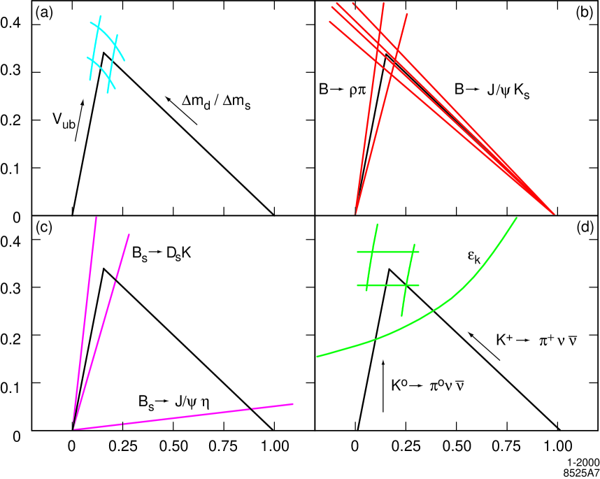
Figure 8: Illustration of four determinations of the unitarity triangle, by (a) non-CP observables, (b) $B$ asymmetries, (c) $B_{s}$ asymmetries, (d) $K$ rare decays. See the text for more details.

Figure 8(a) shows the ‘non-CP triangle’. This triangle takes advantage of the fact that one can determine the unitarity triangle by measuring the absolute values of CKM matrix elements and thus show the existence of the phase through non-CP-violating observables. The left-hand side of the triangle is determined by the rate of $b\to u$ weak decays; the right-hand side is determined by ratio of $B$–$\overline{B}$ mixing amplitudes for $B_{s}$ and $B_{d}$. The rate of $b\to u$ transitions depends only on the CKM matrix element $V_{ub}$ and is not affected by new physics. The $B$ mixing amplitudes involve box diagrams that might have large nonstandard contributions. However, in many models, including models with light supersymmetric particles in which squarks with the same electroweak quantum number are naturally degenerate, these contributions have the same ratio as the standard contributions [52]. Thus, this ‘non-CP triangle’ is the most likely of the four to agree with the true unitarity triangle determined from the CKM matrix.

The expected accuracy that I have displayed in this figure—10% for the $V_{ub}$ side and 5% for the $V_{td}$ side—is surprisingly small, and I would like to defend these estimates now. I will begin with $V_{td}$. This parameter is determined by the relation

$${\Delta m_{d}\over\Delta m_{s}}={m_{Bd}f^{2}_{Bd}B_{Bd}\over m_{Bs}f^{2}_{Bs}B_{Bs}}\cdot\left|{V_{td}\over V_{ts}}\right|^{2}=\xi^{-1}\left|{V_{td}\over V_{ts}}\right|^{2}\ ,$$ (18)

where $f_{Bd}$ is the $B_{d}$ decay constant and $B_{Bd}$ is the matrix element of a 4-fermion operator in the $B_{d}$ wavefunction. The $B_{d}$ mixing parameter $\Delta m_{d}$ is now known to 3.5% accuracy [53]. The $B_{s}$ mixing parameter can be determined by looking for a fast oscillation in tagged $B^{0}$ decays superimposed on the slow oscillation from $B_{d}$ mixing. There is suggestive evidence that such an oscillation appears in the $B$ vertex distribution at the $Z^{0}$, corresponding to an oscillation frequency $\Delta m_{s}\sim 16$ ps^-1 [54]; I have used this value in constructing the figure. Once the oscillation is seen, the frequency can be determined to a few percent. The CDF experiment should be able to make this measurement early in Run II, even for $\Delta m_{s}$ so large that the triangle collapses onto the real axis. Looking back at (18), the magnitude of $V_{ts}$ is constrained by unitarity to be very close to $|V_{cb}|$. Thus, the main source of uncertainty is in the estimation of the $\xi$. The ratio $\xi^{-1}$ is roughly equal to 0.8 and tends to 1 in the chiral limit or in the $SU(3)$ limit $m_{d}=m_{s}$. To achieve 5% accuracy in $\xi$, it is only necessary to compute the deviation of $\xi$ from 1 to 25% accuracy.

Lattice gauge theory should be up to the task. At HEP99, the CP-PACS collaboration reported a calculation [55]

$$\left({f^{2}_{Bd}\over f^{2}_{Bs}}\right)=0.69\cdot(1\pm 7\%\pm 3\%{}^{+5\%}_{-7\%})\ ,$$ (19)

where the three errors come from Monte Carlo statistics, the determination of $m_{s}$, and the continuum extrapolation. It seems to me that, with further effort, a 5% determination of $|V_{td}/V_{cb}|$ is quite feasible. A useful review of the status of lattice gauge theory determinations of these and other heavy-quark matrix elements can be found in [56].

The situation is less clear for $V_{ub}$, but still there is reason for optimism [57]. The best current measurement of $V_{ub}$ is based on the CLEO measurement of the rate of $B\to\rho\ell\nu$ [58],

$$V_{ub}=(3.25\pm 0.14{}^{+0.21}_{-0.29}\pm 0.55)\times 10^{-3}\ ,$$ (20)

where the third contribution to the error represents a 20% spread in the relations given by models between the underlying parameters and the observed rate. The experimental uncertainties are thus quite adequate, and they will decrease in the era of the B-factories. What is needed is a method for computing $V_{ub}$ that has less model uncertainty. Two methods have been proposed. The first is an inclusive technique based on the idea that in a decay $B\to X\ell\nu$, if $m(X)<m_{D}$, then the decay must be a $b\to u$ transition [59, 60]. The problem with this method is that energy from neutral particles cannot be unambiguously associated with a displaced vertex, so one must work with vertex masses based on charged particles and use models to estimate the background from $b\to c$ decays. The DELPHI collaboration has made a promising first application of this technique [61], obtaining

$$V_{ub}=(4.1\pm 0.5\pm 0.6\pm 0.3)\times 10^{-3}\ ,$$ (21)

where the last error indicates a 8% model uncertainty. It is a very interesting question how one defines the optimized vertex mass for this measurement applicable to the B-factory environment. The second method is to measure the spectrum of $B\to\rho\ell\nu$ decays as a function of $m(\ell\nu)$ and evaluate it at the ‘zero-recoil’ point where the heavy $B$ quark decays to a $u$ quark at rest. The value of the form factor at this point can be computed by lattice gauge theory simulations [56].

Figure 8(b) shows the ‘B triangle’. This triangle is constructed from the CP asymmetries in $B^{0}/\overline{B}{}^{0}$ decays. To draw the figure, I have used the asymmetry in $B\to J/\psi K^{0}_{S}$ and the asymmetry in $B\to\rho\pi$. (I ignore the discrete ambiguities in determining the CKM angles from the measured asymmetries.) Both of these asymmetries involve the phase in the $B^{0}$–$\overline{B}{}^{0}$ mixing amplitude and are sensitive to new physics through this source. For $B\to J/\psi K^{0}_{S}$, at least four independent experiments (BaBar, BELLE, CDF, HERA-B) should determine $\sin 2\beta$ an accuracy better than $\pm 0.1$ in the near future. LHC-B or BTeV should determine this parameter to the level of $\pm 0.01$. The constraint from $B\to\rho\pi$ is actually a measurement of $\alpha$ in the CKM picture, but I have moved the constraint to the lower vertex of the triangle for clarity. The process originally thought to best determine $\alpha$, $B\to\pi\pi$, is now disfavored due to potential large background contributions from strong and electromagnetic penguin diagrams. With sufficient statistics, one can fit to the Dalitz plot in $B\to\rho\pi$ to measure and remove these contributions. The BaBar collaboration has estimated an accuracy of $7^{\circ}$ in $\alpha$ for a sample of 600 events [62]. Such a large sample would require luminosities well above the design level. It is also possible to measure $\gamma$ by the comparison of rates for $B^{\pm}\to K^{\pm}D$ decays [63]. This determination involves only tree-level decay amplitudes and so measures the true CKM unitarity triangle rather than the ‘B triangle’.

Figure 8(c) shows the ‘B_s triangle’. The time-dependent CP asymmetry in $B_{s}\to D_{s}^{\pm}K^{\mp}$ is connected to $\sin\gamma$. LHC-B or BTeV should measure $\gamma$ using this reaction to about 10^∘. The $B_{s}$ system also allows an interesting null experiment. The time-dependent CP violation in $B_{s}\to c\overline{c}s\overline{s}$ decays is expected to be very small in the Standard Model. On the other hand, the phase in $B_{s}\to J/\psi\eta$ and $B_{s}\to J/\psi\phi$ should be measurable to a few degrees by LHC-B or BTeV. These reactions will be a very sensitive indicator for new CP violating physics in the $B_{s}$–$\overline{B}_{s}$ mixing amplitude. This constraint is shown, just for the purpose of illustration, as a constraint on the base of the unitarity triangle.

Figure 8(d) shows the ‘K triangle’. This is the triangle determined by the rare $K$ decays $K^{+}\to\pi^{+}\nu\overline{\nu}$, which has an amplitude approximately proportional to $V_{td}$ in the Standard Model, and $K^{0}_{L}\to\pi^{0}\nu\overline{\nu}$, which is a CP-violating process whose amplitude is proportional to Im[$V_{td}$] in the Standard Model. These decays proceed through box diagrams which could well have exotic contributions from new particles with masses of a few hundred GeV. The rare $K$ decays are frighteningly difficult to detect. Experiment E787 at Brookhaven has recently observed 1 event of the $K^{+}$ decay [64]. There are preliminary plans for experiments that would run at Fermilab in the next decay and collect 100 events in each of these rare modes; I have drawn the triangle assuming that these experiments succeed and that their statistical errors are dominant. I have also included in this plot the lower bound of the constraint from $\epsilon$, with conservative errors [62] reflecting the uncertainty in a lattice determination of the overall normalization of hadronic matrix element. It should be noted that, while large deviations from the CKM prediction are possible in rare $K$ decays, broad classes of models give only a relatively small effect [65].

Figure 9 shows the four unitarity triangles superposed on one another. This could well indicate the state of our knowledge of CP violation ten years from now. If the agreement of the various triangles is as good as what is shown here, it will provide striking evidence that the Kobayashi-Maskawa model explains the observed CP violation in weak interactions. But keep in mind the possibility that these four triangles might disagree completely due to loop diagrams involving new heavy particles. We will soon find out which alternative is realized.

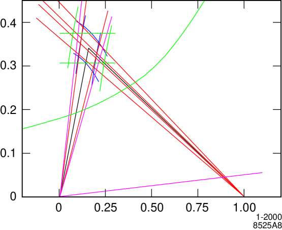
Figure 9: Unitarity triangle determinations from Figure 8 superimposed on a single set of axes.

The HEP99 meeting also saw new theoretical developments in the theory of $B$ meson CP asymmetries. In my discussion of $B\to\rho\pi$ above, I mentioned the difficulties associated with penguin diagrams, which modify the current-current weak interaction and potentially add a different set of phases. It is an important issue in the theory of $B$ decays to provide methods to calculate these penguin contributions or to extract them from data. I would like to highlight three recent pieces of work along these lines. In a presentation at HEP99, Fleischer [66] proposed using $SU(3)$ (more specifically, U-spin) to relate the decay amplitudes for $B\to\pi^{+}\pi^{-}$ and $B_{s}\to K^{+}K^{-}$. Using these relations, it is possible to solve for $\beta$ and $\gamma$ without assumptions about the size of the penguin effects. In another recent paper Neubert and Rosner [67], following up on ideas of Fleischer and Mannel [68], have shown how to extract $\gamma$ without assumptions on the size of the penguin contributions by fitting all partial rate differences among $B^{\pm}\to\pi K$ and $B^{\pm}\to\pi^{\pm}\pi^{0}$ decays. In the most ambitious of these projects, Beneke, Buchalla, Neubert, and Sachrajda [69] reported a new factorization formula applicable to the decays of a $B$ meson to two pseudoscalars meson valid in the formal limit $m_{b}\to\infty$. In perturbative QCD, the leading term in this formula is the naive factorization in which one current from the weak interaction operator creates one final meson. However, the corrections to this term are finite and calculable. A typical result of their method is the formula

$$BR(\overline{B}^{0}\to\pi^{+}\pi^{-}) = 6.5\times 10^{-6}$$ (22)

$$\hskip-42.67912pt\cdot\left|e^{-i\gamma}+0.09e^{-i(13^{\circ})}\right|^{2}\ .$$

On the right-hand side, the prefactor should not be taken seriously, but it can eventually be well determined because it is computed from the same form factor that will be measured in the decay $B\to\pi\ell\nu$. The phase in the second term inside the bracket arises from the imaginary part of a QCD loop diagram. It would be very interesting to understand the accuracy of the formulae obtained by this method, since potentially they make many more processes available for the determination of CKM matrix elements.

Before leaving the subject of CP violation, I would like to remind you that there are many other possible probes which should be explored. Even within the realm of meson asymmetries, there is $D$–$\overline{D}$ mixing, which could have a large CP violating component from sources beyond the Standard Model [70]. Our knowledge of $D$–$\overline{D}$ mixing will be greatly improved by the B factory experiments. Already, CLEO has a new and very impressive limit, which was presented at HEP99 [71]. The neutron and electron electric dipole moments remain important constraints, especially on new angles in supersymmetry that couple to light flavors. CP violation might also be specifically associated with the top quark. The LHC experiments should be able to observe a $10^{-3}$ energy asymmetry between leptons $\ell^{\pm}$ produced in top decays, and this is would be a significant test of CP violation models [72, 73].

Finally, it is important to keep in mind that the Kobayashi-Maskawa model of CP violation cannot provide large enough CP asymmetries to create the baryon/antibaryon asymmetry in the universe [74]. So, we must eventually find a new source of CP violation. It is possible that this source is the mass matrix of heavy leptons, or some other effect at extremely high energy. But it is also possible that the new mechanism of CP violation will appear in the experimental program that we are now beginning to carry out.

4 QCD

We turn next to Quantum Chromodynamics (QCD). In contrast to the previous two topics, the fundamental questions about QCD have been answered already some time ago. The experimental confirmation of QCD as the theory of the strong interactions is now very strong. QCD is now known to account for a wide variety of processes with large momentum transfer, in $e^{+}e^{-}$ annihilation, $ep$ collisions, and $p\overline{p}$ collisions, to about the 10% level of accuracy, and with a common value of the coupling constant $\alpha_{s}$. At the same time, numerical lattice studies confirm that QCD explains the spectrum of light hadrons to about the same level of numerical precision. Wittig has reviewed this latter, less familiar, evidence for QCD at HEP99 [75]. So, what are the important scientific issues for QCD today? I would like to highlight four of these, and give some examples of new work presented at HEP99.

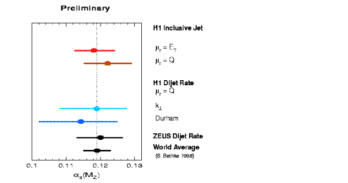
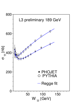
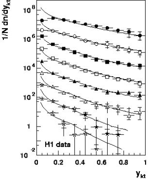
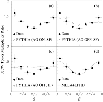
Figure 10: Four figures which show recent experimental advances in QCD. See the text for more details.

The first issue is the precision determination of $\alpha_{s}$. At the moment, the $\overline{M\kern-2.0ptS}$ coupling $\alpha_{s}(m_{Z})$ is known to about 3% accuracy [76]. It is important to reduce this error below 1%. This level of accuracy is needed as an input to the precision experiments of the next decade, for example, the study of the top quark at threshold. It is also already needed to assess the validity of grand unification. I have already noted that grand unification with the renormalization group equations of supersymmetry successfully relates the values of the Standard Model couplings given in (6). In particular, the prediction for $\alpha_{s}$ agrees with experiment at the 10% level, but it is subject at this level to uncertainties from threshold corrections at the scale of grand unification. With a more accurate $\alpha_{s}$, we could evaluate the needed threshold contribution and begin to test explicit models of grand unification. The primary barrier to a more accurate determination of $\alpha_{s}$ come not from experiment (though it would be good to have more precise data on multi-jet rates at energies well above the $Z^{0}$) but rather from theory. However difficult it may be, we need the order $\alpha_{s}^{2}$ corrections to the most important processes which determine $\alpha_{s}$, in particular, the rate for $e^{+}e^{-}\to 3$ jets.

The second issue is the determination of essential strong interaction parameters needed for high energy experiments. Here I mean especially the parton distributions in the proton. Though the quark distributions are well determined, the gluon distribution is not well constrained at moderate values of $x$. This is the freedom that was used to correct the discrepancy between the CDF measurement of the jet rate at large $E_{T}$ and QCD predictions [77]. Gluons at moderate $x$ and low $Q$ evolve to the gluons at low $x$ and high $Q$ which are the dominant source of new particle production at the LHC. The study of high-energy $e^{+}e^{-}$ collisions requires another set of input data, the total cross section for the process $\gamma\gamma\to$ hadrons. It is interesting in its own right to understand what part of this cross section comes from pointlike processes and what part from soft processes involving the hadronic constituents of the photon. The eventual theory should explain, as be constrained by, the data both for $\sigma(\gamma\gamma)$ and $\sigma(\gamma p)$.

The third issue is the study of the detailed structure of jets as predicted by QCD. QCD predicts that the hardest components of jets are built up by successive processes in which gluons or quarks split off from the hardest parton. This gives jets a fractal structure. On top of this backbone, hadrons are produced in a way that reflects the color pairings of the hard partons. If groups of partons are separated in phase space and are separately color neutral, we should find a phase space or rapidity gap in particle production. All of these features are just beginning to be understood from the data.

The fourth issue is one for theorists, the development of new techniques to compute higher-order and multiparton QCD amplitudes. This issue provides essential theoretical support to the first and third topics just listed. At HEP99, Uwer [78], Draggiotis [79], and Harlander [80] set out new ideas for calculational programs whose results should be very interesting.

As an illustration of recent progress in these areas, I present in Figure 10 four of the new QCD results presented at HEP99. The upper left [81] shows that event shape measurements from HERA are now contributing to the precision $\alpha_{s}$ determination. The upper right [82] shows the new determination by L3 of the $\gamma\gamma$ total cross section at LEP. (A similar determination was presented for the $\gamma p$ total cross section at HERA [83].) The large uncertainty, reflected in the difference between the two fits, comes from the fact that about 40% of the total cross section is unobserved, and that theoretical models differ on the size of the contribution from these very soft events. This is a problem that must be addressed. The last two figures show new studies of QCD event shapes. The lower left [84] shows the narrowing of jets with increasing $Q^{2}$ in $ep$ collisions in the H1 event sample. The lower right, from the D0 experiment [85], shows that the particle production in $W+$ jet events reflects the color flow expected for a color singlet $W$ recoiling against a colored parton.

5 Supersymmetry

From the areas of current experimental interest, we now turn to the future. What should be the main topic of discussion at HEP09? What new era in experimental high energy physics will be opening up at that time?

In this section, I would like to take very seriously the second moral I drew in Section 2 from the precision electroweak data. The precision study of the $Z^{0}$ points us toward a world in which the interactions responsible for electroweak symmetry breaking are weakly coupled and the Higgs boson is an elementary scalar particle. I have already explained that some specific aspects of the data are compatible with the idea of supersymmetry at the weak interaction scale. But there is a much stronger argument for the presence of supersymmetry in the fundamental description of Nature. While it is possible in principle that there is no explanation for the negative value of the Higgs (mass)² and the instability to symmetry breaking in the Higgs potential, I insist that we must find a way to explain this instability on the basis of physics. For this, we must have a theoretical framework for the Higgs field in which its potential energy function is calculable. A part of this requirement is that some symmetry must forbid the addition of a Higgs mass term by hand. If the Higgs boson is treated as an elementary field, the only known symmetry with this power is supersymmetry. Thus, to the extent that the precision electroweak data excludes models in which the Higgs is composite or strongly coupled, we should expect to see not a light Higgs boson but also the new particles predicted by supersymmetry.

The idea that the data drives us to a weak-coupling picture of the Higgs boson was controversial at HEP99. Among the people arguing vocally on the other side were Holger Nielsen and Gerard ’t Hooft. So if you do not wish to accept this argument, you are in good company (but still wrong). In any event, for the rest of this lecture I will take this conclusion very seriously and use it to map out future questions for high-energy experimentation.

Among the many theoretical problems connected with supersymmetry, I would like to focus on the spectrum of supersymmetric particles. Supersymmetry predicts that every particle of the Standard Model has a partner with the opposite statistics. That is, the chiral fermions of the Standard Model have scalar partners, and the gauge bosons have spin-$\frac{1}{2}$ (‘gaugino’) partners. What are the masses of these particles?

The interest of this question goes beyond the issue of where or when these particles will be found. To produce a reasonable phenomenology, supersymmetry must itself be spontaneously broken. The supersymmetrized Standard Model cannot directly break supersymmetry, because this hypothesis leads to unwanted very light superpartners [86]. In most models, the description of the superparticle masses involve two ingredients, a sector in which supersymmetry is broken and a ‘mediator’ which connects the symmetry-breaking to the Standard Model fields. The identity of the mediator is typically connected to the very short distance physics of the model, the connection of the Standard Models fields to grand unification or to gravity. And, the nature of the mediator is reflected in the detailed pattern of the masses of superparticles.

If supersymmetry explains the phenomenon of electroweak symmetry breaking, the superparticle masses must have masses of a few hundred GeV; that is, they should be accessible to the experiments of the next decade and possibly even to LEP and the Tevatron. By measuring this mass spectrum, we should, ten years from now, have a wealth of new data which speaks directly to the physics at this fundamental level. It is an exciting prospect. To help you think about it more clearly, I would like to offer a first lesson in superspectroscopy. I will contrast three paradigmatic theories of the mediation of supersymmetry breaking. Though supersymmetry phenomenology has been studied for almost twenty years and went through a period of complacency in the early 1990’s, two of these paradigms were discovered only recently. The second was invented in 1995, and the third only in the past year. Presumably, there are more theoretical insights into this subject that are waiting to be uncovered.

Table 1: Basic formulae for superparticle masses in three paradigms for the spectrum. In this table, $i=1,2,3$ refers to a factor of the gauge group $U(1)\times SU(2)\times SU(3)$, $\alpha_{i}$ is the gauge coupling evaluated at $m_{Z}$, $\alpha_{U}$ is the unification coupling, $C_{i}$ is the squared gauge charge, and $f$ refers to a chiral quark or lepton flavor. The renormalization group functions of the supersymmetric Standard Model are notated: $\beta_{i}=-b_{i}g_{i}^{3}/(4\pi)^{2}$, $\gamma_{f}=-\eta_{fi}g_{i}^{2}/(4\pi)^{2}$. In the gauge mediation line, the factor 2 in the scalar mass formula is actually model-dependent.

	Gaugino $m^{2}$	Scalar $m^{2}$
Gravity	$\displaystyle{{\alpha_{i}^{2}\over\alpha_{2}^{2}}m_{2}^{2}}$	$\displaystyle{m_{0}^{2}+\sum_{i}2C_{i}{\alpha_{i}^{2}-\alpha_{U}^{2}\over b_{i}\alpha_{2}^{2}}m_{2}^{2}}$
Gauge	$\displaystyle{{\alpha_{i}^{2}\over\alpha_{2}^{2}}m_{2}^{2}}$	$\displaystyle{\sum_{i}2C_{i}{\alpha_{i}^{2}\over\alpha_{2}^{2}}m_{2}^{2}}$
Anomaly	$\displaystyle{{b_{i}^{2}\over b_{2}^{2}}{\alpha_{i}^{2}\over\alpha_{2}^{2}}m_{2}^{2}}$	$\displaystyle{\sum_{i}2\eta_{fi}b_{i}{\alpha_{i}^{2}\over\alpha_{2}^{2}}m_{2}^{2}}$

The three paradigms for the superspectrum that I would like to discuss are those of ‘gravity mediation’, ‘gauge mediation’, and ‘anomaly mediation’. In gravity mediation, as introduced in [87, 88, 89], the mediator is supergravity itself. One imagines a sector that spontaneously breaks supersymmetry. Let $m_{\mbox{\scriptsize Pl}}$ be the Planck scale. Then the gaugino masses arise from direct order $1/m_{\mbox{\scriptsize Pl}}$ couplings of this sector to the Standard Model Yang-Mills Lagrangian, and scalar masses arise from direct order $1/m_{\mbox{\scriptsize Pl}}^{2}$ couplings of this sector into the Standard Model potential. If the superparticle masses are of the order of the weak scale, the mass of the gravitino is of the same order. The spectrum acquires additional structure from the renormalization group evolution of the mass parameters from the Planck scale to the weak scale.

In gauge mediation, introduced in [90], the mediator is the supersymmetric version of the Standard Model gauge interactions. One imagines that supersymmetry is broken by a new sector which includes heavy particles with Standard Model gauge couplings. Then gaugino masses arise from one-loop diagrams involving these heavy particles, and scalar masses arise from two-loop diagrams in which the loop of heavy particles appears in a scalar self-energy diagram. Because what is computed for scalars is the (mass)², both gauginos and scalars acquire masses of order $\alpha$ with respect to the heavy scale. The gravitino has a mass of order eV and is typically the lightest superparticle. Other superparticles may be observed to decay to the gravitino if the rate of this decay is not suppressed by a very large value of the heavy mass.

Anomaly mediation, introduced in [91, 92] represents the opposite extreme pole. To realize this possibility, one considers models in which the supergravity couplings needed to work gravity mediation vanish. Then the partners of Standard Model particles acquire no mass at tree level. In this case, it turns out that the first mass contribution is universal in character and is connected to the breaking of scale invariance by the running of the Standard Model coupling constants. The gravitino mass does arise at the tree level, and so in this scheme the gravitino mass is about 100 TeV if the Standard Model superparticles acquire weak scale masses.

In Table 1, I have collected the basic formulae for the gaugino and scalar masses in these three paradigms. For clarity, I have eliminated the underlying parameters in terms of the mass $m_{2}$ of the $W$ boson superpartner. In the case of gravity mediation, there is another independent parameter $m_{0}$. For gauge mediation and anomaly mediation, the superparticle masses naturally depend only the Standard Model quantum numbers, a feature that suppresses new flavor-changing neutral current effects from supersymmetry loop diagrams. This property also holds in gravity mediation in the ‘no-scale’ limit $m_{0}\to 0$. Away from this limit, there is no clear reason why $m_{0}$ should not depend on flavor except that this could lead to unwanted neutral current effects.

Anomaly mediation makes two specific predictions that deserve comment. First, the lightest gaugino are expected to be an almost degenerate $SU(2)$ triplet $\widetilde{w}^{\pm}$, $\widetilde{w}^{0}$, with the charged states only a few hundred MeV above the neutral one [94]. This gives rise to a distinctive phenomenology, discussed in [95, 96, 97]. Second, the scalars partners of leptons are computed to have negative (mass)², a disaster. Some cures for this problem are given in [98, 99].

In Figure 11, I show a comparison of the spectra for the three paradigms; for gravity mediation, I give both the ‘no-scale’ case $m_{0}=0$ and the case $m_{0}/m_{2}=5$ and universal.

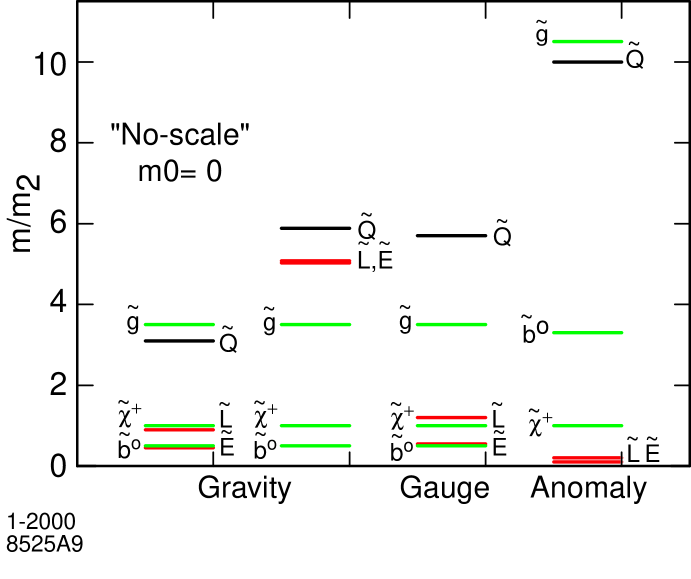
Figure 11: Spectra of superparticles in two cases of gravity mediation, gauge mediation, and anomaly mediation, according to the formulae of Table 1.

I emphasize that the formulae in Table 1 represent only the first lesson in superspectroscopy. They omit possible mass mixings and effects of large top, bottom, and $\tau$ Yukawa couplings, and they omit higher-order corrections [93]. Nevertheless, these formulae and Figure 11 already give a feeling for the complexity of the spectrum that might be found when superparticles appear in experiments.

If supersymmetry is the explanation of electroweak symmetry breaking, it is likely that the LHC will be able to sample the whole superparticle mass spectrum, including the heaviest states. In addition, as members of the ATLAS collaboration have recently demonstrated, the LHC experiments have the ability to make precision measurements of superparticle masses in a number of different scenarios [100]. Nevertheless, the richness of the phenomena calls for the exploration of these particles also in $e^{+}e^{-}$ annihilation. It is worth remembering that an $e^{+}e^{-}$ linear collider of the next generation will provide not only a relatively clean environment with kinematic constraints that aid in particle mass measurements, but also the availability of beam polarization, which is very useful in resolving questions of particle mixing [101]. The production cross sections for superparticles are electroweak and can be computed precisely, allowing an unambiguous determination of the quantum numbers of each new particle.

The superspectrum is complex, but the LHC and linear collider are powerful instruments. With these two facilities, with their complementary strengths, we could fully explore the supersymmetry spectrum of particles and mine the information it contains for information about a truly fundamental level of physics. This is already cause for optimism about the future of experimental particle physics. But, there is more.

6 New space dimensions

Many people say that the key problem of quantum physics has nothing to do with what we do at accelerators. Rather, they say, it is the problem of the compatibility of quantum mechanics with general relativity. To solve this problem, one must do two things, first, remove the divergences from the quantum theory of gravity, and, second, unify gravity with the microscopic particle interactions.

Most people who recite this litany do not realize that we have at least one possible solution already in hand. It is string theory. String theory has not been proved to be the correct theory of Nature, but it does demonstrably solve these two problems. It is the only known approach to these problems which has no glaring weaknesses. Therefore, we must take it very seriously.

There has been tremendous progress in string theory since the 1995 discovery of string dualities by Hull and Townsend [102] and Witten [103]. Just in the past year, two new and very profound ideas have been validated: The first is the idea of ‘t Hooft [104] and Susskind [105] that quantum gravity is ‘holographic’, in the sense that its physical degrees of freedom are those of a manifold with one lower dimension that the dimension of space time. The second is an explicit realization of this relation, due to Maldacena [106], a duality linking supersymmetric Yang-Mills theory in 4 dimensions with supergravity in 5-dimensional anti-de Sitter space. I do not have space here to do justice to these ideas, but they are described clearly in Bachas’ lecture at HEP99 [107].

I would like to concentrate instead on another consequence of the new understanding of string dualities. These developments have led to new classes of models in which quantum gravity and string physics is much more accessible to experiment and may even appear directly in the realm of the LHC and the linear collider.

String theory requires that we live in a world which has 11 dimensions. Until recently, it was thought that this could only be compatible with our observations if seven of these dimensions were compact and very small, of the order of the Planck scale. It is interesting, though, to think about new space dimensions that are not so small. In 4 dimensions, the gravitational force falls off as

$$F\sim{m_{1}m_{2}\over r^{2}}\ ;$$ (23)

in $(4+n)$ dimensions, it falls off as

$$F\sim{m_{1}m_{2}\over r^{2+n}}\ .$$ (24)

Consider the $n$ extra dimensions to be periodic with period $2\pi R$. Then two masses separated by a distance much larger than $R$ would feel a gravitational force of the form (23), while two masses separated by a distance much less than $R$ would feel a gravitational force of the form (24). The short-distance force is the more fundamental. We can define the fundamental quantum gravity scale $M$ by writing the dimensionful constant of proportionality in (24) as a numerical constant times $M^{-(n+2)}$. The constant of proportionality in (23) is just Newton’s constant. If we insist that the forces match at the distance scale $R$, we obtain the relation

$$(4\pi G_{N})^{-1}=R^{n}M^{n+2}\ .$$ (25)

This equation has a surprising implication. If we fix $G_{N}$ to its observed value and imagine larger values of $R$, then the true fundamental quantum gravity scale becomes smaller.

How large could $R$ be? In principle, $R$ could vary continuously. But there are four natural choices represented in the literature as explicit classes of models. Using a standard American nomenclature, these sizes are:

1. micro-: In this case, all three quantities in (25) are of the order of $M_{\mbox{\scriptsize Pl}}$. This is the original proposal of Scherk and Schwarz for the size of extra dimensions in string theory [108].

2. mini-: In this case, $M$ is taken to be of the order of the grand unification scale, $2\times 10^{16}$ GeV. In fact, Hořava and Witten [109] have argued that there is a solution in which all fundamental scales in Nature are of order the grand unification scale, with the scale of the 11th dimension only a small amount larger. This theory includes the unification of Standard Model couplings provided by supersymmetry, and a unification with gravity as well.

3. midi-: In this case, $R$ is taken to be at the TeV scale. From (25), for $n=6$ for example, the fundamental gravity scale $M$ would be 8000 TeV. This choice was first advocated by Antoniadis [110], who showed how it could lead to superparticle masses of the order of the weak interaction scale. It is possible to arrange a unification of Standard Model couplings at the scale $M$ [111]. Recently, Randall and Sundrum [112] have presented a 5-dimensional model with curvature in the extra dimension which gives a novel way to relate the Planck scale and the TeV scale. The phenomenology of this model is quite similar to that of models with flat extra dimensions of TeV-scale size [113].

4. maxi-: In this case, $M$ is taken to be at the TeV scale. Then $R$ would be at some scale from millimeters ($n=2$) to fermi ($n=7$). These large distances, which are huge on the scale of high-energy physics, would seems to violate common sense. But Arkani-Hamed, Dimopoulos, and Dvali [114] have argued that this aggressive choice is not excluded. In this case, the quantum gravity scale $M$, the shortest possible distance in Nature, might already be accessible to accelerator experiments.

The maxi- case requires one extra condition. From tests of Bhabha scattering and fermion pair production at LEP and quark-antiquark scattering at the Tevatron, we know that the strong, weak, and electromagnetic interactions follow the force laws predicted for four dimensions up to momentum transfers of about 1 TeV. This means that the quarks, leptons, and gauge bosons must be confined to a 4-dimensional submanifold of thickness less than 1/TeV inside the new large dimensions. This is known to be possible in string theory. Indeed, string theory contains a classical solution called a ‘D-brane’, which can have fermions, bosons, and gauge fields bound to its surface [115, 116]. In the maxi- case, the Standard Model particles would live on a D-brane, whose thickness would be of order $1/M$, while gravity and perhaps other light fields could propagate in the full space, out to distances of order $R$. A picture of this construction is given in Figure 12.

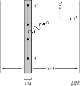
Figure 12: Picture of the universe viewed in the small, with quarks, leptons, and gauge fields bound to a D-brane localized in an extra compact dimension.

The micro- case above is famously difficult to test and has given rise to unfortunate statements that string theory is not physics. But I would like to argue now that the other three cases are amenable to experimental test, and that in fact they can be tested at the LHC and the linear collider. Indeed, ten years from now, we could be arguing from experimental data about the true number of space dimensions in Nature.

I will discuss the three cases in turn, from large to small. Consider first the maxi-scale case. One might think that such large extra dimensions are excluded by Cavendish experiments, but actually the best current limit is only $R<0.8$ mm ($M>940$ GeV) [117]. More significant constraints come from searches for quantum gravity effects at accelerators. Two methods have been proposed. The first is to search for processes in which a collision causes a graviton to be radiated off the brane, carrying with it unobserved momentum [118, 119]. The simplest processes of this kind are

$$e^{+}e^{-}\to\gamma G\ ,\qquad q\overline{q}\to gG\ ,$$ (26)

where $G$ is a graviton, and these can be observed as missing energy processes at $e^{+}e^{-}$ and hadron colliders. I will discuss the experimental status of this search in a moment. The second is to search for a contact interaction in fermion-fermion reactions due to graviton exchange [118, 120, 121]. The coefficient of the induced contact interaction is model-dependent, to one cannot use this effect to set strict limits on $M$. But if the effect were there, it would be striking, causing the cross sections in $e^{+}e^{-}\to f\overline{f}$ to bend upward as a function of energy, and also modifying the production angular distributions. There is new data from LEP on the pair-production total cross sections, but, unfortunately for this purpose, it is in remarkable agreement with the Standard Model prediction. The new data from DELPHI is shown in Figure 13 [122].

Figure 13: Total cross sections for fermion pair production in $e^{+}e^{-}$ annihilation at LEP energies, from [120].

On the other hand, the cross sections for missing-energy processes can be computed absolutely in terms of the gravity scale defined by (25) and the number of extra dimensions $n$, so that bounds on these processes allow us to place lower bounds on $M$. In Table 2, taken from [123], I give the best current limits on $M$ (at 95% confidence) from LEP and the Tevatron and the sensitivity expected at LHC and at a 1 TeV linear collider. The LEP results correspond to new limits announced at HEP99 [124]. The first line of the table gives a set of bounds from an astrophysical source, the constraint that supernova 1987A did not radiate away most of its energy in gravitons [125]. This bound is very strong for $n=2$ but is unimportant for larger $n$. I exclude cosmological bounds that are really constraints on the cosmological scenario.

Table 2: Current and future sensitivities to large extra dimensions from missing-energy experiments. All values for colliders are expressed as 95% confidence limits on the size of extra dimensions $R$ (in cm) and the effective Planck scale $M$ (in GeV). For the analysis of SN1987A, we give probable-confidence limits.

Collider		R / M ($n=2$)	R / M ($n=4$)	R / M ($n=6$)
Present:	SN1987A	$3\times 10^{-5}/50000$	$1\times 10^{-9}/1000$	$6\times 10^{-11}/100$
	LEP 2	$4.8\times 10^{-2}$ / 1200	$1.9\times 10^{-9}$ / 730	$6.8\times 10^{-12}$ / 530
	Tevatron	$5.5\times 10^{-2}$ / 1140	$1.4\times 10^{-9}$ / 860	$4.1\times 10^{-12}$ / 780
Future:	LC	$1.2\times 10^{-3}$ / 7700	$1.2\times 10^{-10}$ / 4500	$6.5\times 10^{-13}$ / 3100
	LHC	$4.5\times 10^{-4}$ /12500	$5.6\times 10^{-11}$ / 7500	$2.7\times 10^{-13}$ / 6000

In Table 2, the sensitivity to missing-energy processes expected at the LHC is quite remarkable. These values cannot be completely trusted, for the usual reason that the LHC cross sections integrate over very large momentum transfer processes. However, it is argued in [123] that the values in the Table are most likely to underestimate the LHC sensitivity. It was the original idea of Arkani-Hamed, Dimopoulos, and Dvali that the size of the weak interaction scale should be set by the scale of $M$. The LHC search for missing energy processes should provide a sensitive test of this hypothesis.

I should note that the maxi- case throws away the grand unification scale and all of the physics associated with it. This includes the unification of coupling constants through the renormalization group. It also includes the suppression of neutrino masses and proton decay matrix elements by the factor $m_{W}/M_{\mbox{\scriptsize GUT}}$, a factor that arises naturally in the standard picture from the fact that these effects are mediated by dimension 5 operators. New suppression mechanisms are needed if we have large extra dimensions. Actually, this may be less a problem than an opportunity to discover new physical mechanisms; see [126] for an example.

We turn next to the midi- case. In this class of models, the Standard Model fields can consistently explore the extra dimensions. Direct quantum gravity effects are inaccessible, but we should expect to see the excitation of states of the photon, $Z^{0}$, and gluon with nonzero momentum in the extra dimensions. These states appear in experiment as massive vector resonances, called ‘Kaluza-Klein recurrences’. If the extra dimensions are flat and have periodicity $2\pi R$, the masses of the these states are $|\vec{N}|/R$, where $\vec{N}$ is a vector with integer components. The spectrum of Kaluza-Klein recurrences is a Fourier transform of the shape of the extra dimensions [127, 128]. Figure 14 shows the effect of these recurrences in producing resonances in the dilepton invariant mass distribution that would be observed at the LHC.

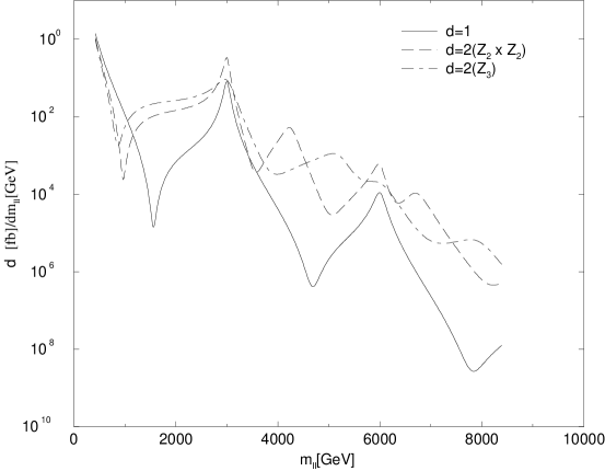
Figure 14: Dilepton mass spectra expected at the LHC due to Kaluza-Klein recurrences of the photon and $Z^{0}$, for $1/R=3$ TeV, from [125]. The solid curve is computed for one compactified dimension, the dashed curves for two cases of two compactified dimensions.

Finally, we come to the mini- case. In this class of models, the direct effects of the extra dimensions occur only at the grand unification scale and cannot be observed experimentally. A test of the hypothesis would have to be based on a characteristic set of Lagrangian parameters following from the geometry. These parameters would provide a boundary condition for the renormalization group equations, and we would compare the results of integrating those equation to the weak interaction scale with the results of our experiments.

Here is a concrete picture of how such a comparison could be made. In the original model of Hořava and Witten [109], the geometry of Nature is effectively five-dimensional and has the form shown in Figure 15. The fifth dimension is bounded, and gauge bosons, fermions, and scalars are bound to four-dimensional walls at the boundary of the space. On one wall, we would have the supersymmetric Standard Model. What is on the other wall? Hořava and Witten [109] proposed that this would be a natural place to put the hidden sector responsible for supersymmetry breaking.

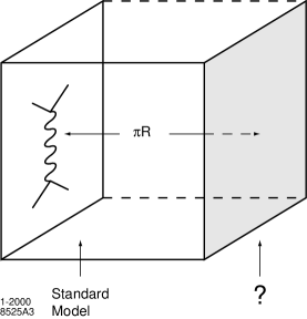
Figure 15: Picture of the universe viewed in the small following the ideas of Hořava and Witten. There is an extended fifth dimension, with quarks, leptons, and gauge fields bound to a wall on one boundary of the space.

We must now ask, what supersymmetry spectrum follows from this hypothesis? Two answers have been given in the literature. Hořava [129] has argued that one should find the spectrum of gravity mediation in the no-scale limit. However, this result has been criticized by Nilles, Olechowski, and Yamaguchi [130], who have found large contributions to $m_{0}$ in his picture. Randall and Sundrum [92] have argued that one should find the spectrum of anomaly mediation. However, we have already seen that that spectrum is not self-consistent and requires correction to produce positive slepton masses. Despite these problems with the answers that have been proposed up to now, I believe that the question I have asked has a definite answer, and many theorists are now working to find it. If someone succeeds, the result will give a remarkable and concrete goal for the experimental studies of supersymmetry spectroscopy that we are soon to undertake.

7 Lutheran sermon

Tampere has a number of beautiful stone churches, and, in touring them, we learned that sermons play an important role in the Finnish Lutheran traditions. So I will conclude with a sermon.

For me, the most memorable part of the HEP99 meeting was a formal ceremony conducted by four young physicists representing the four LEP collaborations—Fabio Cerutti, Magali Grüwe, Simonetta Gentile, and Mario Pimenta. The title of the ceremony was: ‘Any sign of New Physics in the 1999 LEP data?’. The speakers were thorough, precise, and extremely well-informed. The answer to the question in the title was, no.

It is wrong to be cynical about such an exercise, but it is correct to be disappointed. These speakers stood at the apex of a huge superstructure, representing more than a billion dollars of investment in equipment and training, all focused on the goal of breaking through to the next layer of physics beneath the strong, weak, and electromagnetic interactions. This time, we did not succeed. What moral should we draw from this?

Most of the people in my audience for this lecture were still in grammar school in the 1970’s. This was a very different era in high energy physics, with surprising discoveries and puzzles coming from experiment, forming a cloudy picture in which one struggled to the see the final outcome. I was a graduate student in that period, and the excitement drew me in, away from a perhaps more sensible career in the physics of materials. We do not feel this sort of excitement in high-energy physics today, and many people now ask if it will ever return.

On the other hand, it is important to recognize that the experimental progress we have made in the 1990’s is remarkable in another way. It was often said in the early 1970’s that the experimental picture was necessarily unclear, because we were exploring a realm very remote from human experience. Here I do not refer to the requirement that high energy phenomena need to be observed by complex detectors, but to the conceptual problem of visualizing the basic objects that were used to construct theories—quarks, gluons, heavy bosons, and the like. It was thought that we could view these objects only indirectly, by matching experimental results to abstruse theoretical predictions.

In the 1990’s we learned that this attitude is hogwash. Quarks and leptons may be unimaginably small, but with the right experiments, we can reveal all of the fine details of their behavior. Especially through the program of precision experiments at the $Z^{0}$ resonance, we have been able to examine the quarks or leptons of each individual species, shake their hands, and watch their dances. However remote this microworld is, we understand it pictorially, and with certainty. It is important to add that the means by which we have achieved this understanding is that of using accelerators to go to the basic scale on which these objects act, and then looking and seeing what is manifest there.

In the process, we have learned that physics at this microscopic scale has a basis as rational as chemistry. Quarks and leptons move, not by magic, but because there is a mechanism at work. Experimentally, we have found the moving parts and exhibited their properties. This understanding is very encouraging for the major unsolved aspects of the behavior of the Standard Model, the breaking of electroweak gauge symmetry. This phenomenon must also have a cause, and our experience in the 1990’s tells us that, if we can patiently continue our investigations to higher energy, we can find it out.

The idea that there are mechanisms and reasons for physical phenomena, and that we can find the next one by searching to smaller distances, is an article of faith. As our experimental devices become more complex and expensive, and as the time required to realize them stretches out, it becomes harder and harder to keep the faith. The public wants results on the nightly news. Our allies in government work on the time scale of an election cycle; our colleagues in industry measure progress in ‘Internet time’. It requires continuing effort to persuade them that, though our enterprise moves much more slowly, it is in motion, and toward important goals. But our hardest struggle is with ourselves and our community, to press on to the next great period of discovery which is still over the horizon.

In talking to many people in the experimental community, I sense a pessimism, not about whether there is a next scale of physics, but about what we will find there. Just the Standard Model, they say, just the Higgs boson, just the familiar pattern that some theorist has set out. The excitement of the 1970’s has receded very far into the past, so far that it is difficult to imagine that it will come again.

This is the reason that I have given so much attention in this lecture to the possibility of new space dimensions. Though I have tried to motivate this idea, I think that its major importance comes not so much because it must be true as because it gives an example of how much we could have to learn, and how profoundly different the deep structure of the universe could be from what we now conceive. There could really be unguessed secrets in the laws of Nature. And, these secrets are not hiding in the cosmos or on the large scales of the universe, and not in rare materials or the organization of matter, but only at very small distances.

This is where our accelerators will take us, if we can marshall our resources and our intellectual strength. Above all, we have to keep our belief in our joint enterprise, the belief that Nature has more wonders, beyond our imagination, which wait patiently for our tools to reach them.

I am grateful to Profs. Wolfgang Kummer and Matts Roos and to the members of the HEP99 organizing committee for giving me the opportunity to present this lecture, and to colleagues too numerous to mention, both at SLAC and at HEP99, who have helped me to understand the topics discussed here. I thank particularly Adam Falk, Yuval Grossmann, and Zoltan Ligeti for discussions of CP violation. My work is supported by the US Department of Energy under contract DE–AC03–76SF00515.

References

- [1] L. Foa, these proceedings.
- [2] G. Altarelli, in Proceedings of the 1989 International Symposium on Lepton and Photon Interactions at High Energies, M. Riordan, ed. (World Scientific, 1990).
- [3] A. Sirlin, Phys. Rev. D22, 971 (1980); W. J. Marciano and A. Sirlin, Phys. Rev. D22, 2695 (1980).
- [4] J. Ellis and G. L. Fogli, Phys. Lett. B231, 189 (1989). Phys. Lett. B232, 139 (1989).
- [5] A. Weidberg, in Proceedings of the 1989 International Symposium on Lepton and Photon Interactions at High Energies, M. Riordan, ed. (World Scientific, 1990).
- [6] M. K. Campbell, ibid.
- [7] G. Feldman, ibid.
- [8] M. E. Peskin and T. Takeuchi, Phys. Rev. Lett. 65, 964 (1990), Phys. Rev. D46, 381 (1992).
- [9] W. J. Marciano and J. L. Rosner, Phys. Rev. Lett. 65, 2963 (1990).
- [10] G. Altarelli and R. Barbieri, Phys. Lett. B253, 161 (1991); G. Altarelli, R. Barbieri, and S. Jadach, Nucl. Phys. B369, 3 (1992).
- [11] M. L. Swartz, in Proceedings of the 1999 International Symposium on Lepton and Photon Interactions at High Energies, J. Jaros and M. E. Peskin, eds. (World Scientific, 2000), hep-ex/9912026.
- [12] A. Sirlin, ibid., hep-ph/9912227.
- [13] J. Mnich, these proceedings.
- [14] R. S. Chivukula, S. B. Selipsky and E. H. Simmons, Phys. Rev. Lett. 69, 575 (1992), hep-ph/9204214; R. S. Chivukula, E. H. Simmons and J. Terning, Phys. Lett. B331, 383 (1994), hep-ph/9404209.
- [15] Y. Zhu, these proceedings.
- [16] J. F. Gunion, H. E. Haber and J. Wudka, Phys. Rev. D43, 904 (1991).
- [17] T. Appelquist and J. Terning, Phys. Lett. B315, 139 (1993), hep-ph/9305258; T. Appelquist, J. Terning and L. C. Wijewardhana, Phys. Rev. Lett. 79, 2767 (1997), hep-ph/9706238.
- [18] P. Langacker and N. Polonsky, Phys. Rev. D52, 3081 (1995), hep-ph/9503214; D. M. Pierce, in Proceedings of the 1997 SLAC Summer Institute, A. Breaux, J. Chan, L. DePorcel, and L. Dixon, eds. (SLAC, 1998), hep-ph/9701344.
- [19] T. Moroi and Y. Okada, Phys. Lett. B295, 73 (1992).
- [20] G. L. Kane, C. Kolda and J. D. Wells, Phys. Rev. Lett. 70, 2686 (1993), hep-ph/9210242.
- [21] J. R. Espinosa and M. Quiros, Phys. Lett. B279, 92 (1992), Phys. Lett. B302, 51 (1993), hep-ph/9212305.
- [22] E. Gross, these proceedings.
-
[23]
M. Roco, these proceedings; M. Carena, et al.,
http://fnth37.fnal.gov/higgs.html. - [24] D. Buskulic et al. [ALEPH Collaboration], Z. Phys. C69, 183 (1996).
- [25] K. Abe et al. [SLD Collaboration], Phys. Rev. Lett. 81, 942 (1998).
- [26] OPAL Collaboration, OPAL Physics Note 358, submitted to the 1998 International Conference on High-Energy Physics.
- [27] L3 Collaboration, L3 Note 2378, submitted to EPS-HEP99; M. Acciarri et al. [L3 Collaboration], Phys. Lett. B474, 194 (2000), hep-ex/0001016.
- [28] J. H. Christenson, J. W. Cronin, V. L. Fitch and R. Turlay, Phys. Rev. Lett. 13, 138 (1964).
- [29] L. Wolfenstein, Phys. Rev. Lett. 13, 562 (1964).
- [30] M. Kobayashi and T. Maskawa, Prog. Theor. Phys. 49, 652 (1973).
- [31] S. Weinberg, Phys. Rev. Lett. 37, 657 (1976).
- [32] F. J. Gilman and M. B. Wise, Phys. Lett. B83, 83 (1979).
- [33] H. Burkhardt, et al. [NA31 Collaboration], Phys. Lett. B206, 169 (1988).
- [34] J. R. Patterson, et al., Phys. Rev. Lett. 64, 1491 (1990).
- [35] V. Fanti et al. [NA48 Collaboration], Phys. Lett. B465, 335 (1999), hep-ex/9909022.
- [36] A. Alavi-Harati et al. [KTeV Collaboration], Phys. Rev. Lett. 83, 22 (1999) hep-ex/9905060.
- [37] G. Buchalla, these proceedings, hep-ph/9912369.
- [38] A. Buras, M. Jamin and M. E. Lautenbacher, Nucl. Phys. B408, 209 (1993), hep-ph/9303284. S. Bosch, A. J. Buras, M. Gorbahn, S. Jager, M. Jamin, M. E. Lautenbacher, and L. Silvestrini, hep-ph/9904408.
- [39] J. M. Flynn and L. Randall, Phys. Lett. B224, 221 (1989).
- [40] J. F. Donoghue and E. Golowich, hep-ph/9911309.
- [41] A. Soni, these proceedings.
- [42] D. B. Kaplan, Phys. Lett. B288, 342 (1992), hep-lat/9206013.
- [43] Y. Shamir, Nucl. Phys. B406, 90 (1993), hep-lat/9303005.
- [44] T. Blum and A. Soni, Phys. Rev. D56, 174 (1997), hep-lat/9611030, Phys. Rev. Lett. 79, 3595 (1997), hep-lat/9706023.
- [45] A. B. Carter and A. I. Sanda, Phys. Rev. Lett. 45, 952 (1980), Phys. Rev. D23, 1567 (1981); I. I. Bigi and A. I. Sanda, Nucl. Phys. B193, 85 (1981).
- [46] G. Bauer, these proceedings, hep-ex/9908055; T. Affolder et al. [CDF Collaboration], hep-ex/9909003.
- [47] J. D. Bjorken, Phys. Rev. D39, 1396 (1989).
- [48] C. Jarlskog and R. Stora, Phys. Lett. B208, 268 (1988).
- [49] Y. Nir and D. J. Silverman, Nucl. Phys. B345, 301 (1990).
- [50] A. G. Cohen, D. B. Kaplan, F. Lepeintre and A. E. Nelson, Phys. Rev. Lett. 78, 2300 (1997), hep-ph/9610252.
- [51] Y. Grossman, Y. Nir and M. P. Worah, Phys. Lett. B407, 307 (1997), hep-ph/9704287.
- [52] J. L. Hewett, T. Takeuchi and S. Thomas, in Electroweak Symmetry Breaking and Beyond the Standard Model, T. Barklow, S. Dawson, H. Haber, and J. Siegrist, eds. (World Scientific, 1996), hep-ph/9603391.
- [53] M. Artuso, these proceedings, hep-ph/9911347.
- [54] G. Blaylock, in Proceedings of the 1999 International Symposium on Lepton and Photon Interactions at High Energies, J. Jaros and M. E. Peskin, eds. (World Scientific, 2000), hep-ex/9912038.
- [55] H. P. Shanahan [CP-PACS Collaboration], these proceedings, hep-ph/9909398.
- [56] S. Aoki, in Proceedings of the 1999 International Symposium on Lepton and Photon Interactions at High Energies, J. Jaros and M. E. Peskin, eds. (World Scientific, 2000), hep-ph/9912288.
- [57] Z. Ligeti, hep-ph/9908432.
- [58] B. H. Behrens et al. [CLEO Collaboration], hep-ex/9905056.
- [59] V. Barger, C. S. Kim and R. J. Phillips, Phys. Lett. B251, 629 (1990).
- [60] J. Dai, Phys. Lett. B333, 212 (1994), hep-ph/9405270.
- [61] P. Collins [DELPHI Collaboration], Nucl. Phys. Proc. Suppl. 75B, 288 (1999).
- [62] P. F. Harrison, H. R. Quinn, et al. [BABAR Collaboration], The BaBar Physics Book, SLAC-R-0504.
- [63] D. Atwood, I. Dunietz and A. Soni, Phys. Rev. Lett. 78, 3257 (1997), hep-ph/9612433.
- [64] S. Adler et al. [E787 Collaboration], Phys. Rev. Lett. 79, 2204 (1997), hep-ex/9708031.
- [65] Y. Nir and M. P. Worah, Phys. Lett. B423, 319 (1998), hep-ph/9711215.
- [66] R. Fleischer, these proceedings, hep-ph/9908341, hep-ph/0001253.
- [67] M. Neubert and J. L. Rosner, Phys. Lett. B441, 403 (1998), hep-ph/9808493, Phys. Rev. Lett. 81, 5076 (1998), hep-ph/9809311.
- [68] R. Fleischer and T. Mannel, Phys. Rev. D57, 2752 (1998), hep-ph/9704423.
- [69] M. Beneke, these proceedings, hep-ph/9910505; M. Beneke, G. Buchalla, M. Neubert and C. T. Sachrajda, Phys. Rev. Lett. 83, 1914 (1999), hep-ph/9905312.
- [70] G. Blaylock, A. Seiden and Y. Nir, Phys. Lett. B355, 555 (1995), hep-ph/9504306.
- [71] M. Palmer, these proceedings; R. Godang [CLEO Collaboration], hep-ex/0001060.
- [72] C. R. Schmidt and M. E. Peskin, Phys. Rev. Lett. 69, 410 (1992); C. R. Schmidt, Phys. Lett. B293, 111 (1992).
- [73] W. Bernreuther and A. Brandenburg, Phys. Lett. B314, 104 (1993), Phys. Rev. D49, 4481 (1994), hep-ph/9312210.
- [74] P. Huet and E. Sather, Phys. Rev. D51, 379 (1995), hep-ph/9404302.
- [75] H. Wittig, these proceedings, hep-ph/9911400.
- [76] J. Womersley, in Proceedings of the 1999 International Symposium on Lepton and Photon Interactions at High Energies, J. Jaros and M. E. Peskin, eds. (World Scientific, 2000), hep-ex/9912009.
- [77] J. Huston, E. Kovacs, S. Kuhlmann, H. L. Lai, J. F. Owens, D. Soper and W. K. Tung, Phys. Rev. Lett. 77, 444 (1996), hep-ph/9511386; H. L. Lai et al., Phys. Rev. D55, 1280 (1997), hep-ph/9606399.
- [78] D. A. Kosower and P. Uwer, Nucl. Phys. B563, 477 (1999), hep-ph/9903515.
- [79] P. Draggiotis, R. H. Kleiss and C. G. Papadopoulos, Phys. Lett. B439, 157 (1998), hep-ph/9807207.
- [80] K. G. Chetyrkin, R. Harlander, T. Seidensticker and M. Steinhauser, these proceedings, hep-ph/9910339.
- [81] T. Carli [H1 Collaboration], hep-ph/9910360.
- [82] S. Costantini, these proceedings; L3 Collaboration, L3 Note 2400, submitted to EPS-HEP99.
- [83] C. Amelung [ZEUS Collaboration], hep-ex/9911005.
- [84] C. Adloff et al. [H1 Collaboration], hep-ex/9912052.
- [85] N. Varelas, these proceedings; D0 Collaboration, paper 163E submitted to EPS-HEP99.
- [86] S. Dimopoulos and H. Georgi, Nucl. Phys. B193, 150 (1981).
- [87] A. H. Chamseddine, R. Arnowitt and P. Nath, Phys. Rev. Lett. 49, 970 (1982), Nucl. Phys. B227, 121 (1983).
- [88] R. Barbieri, S. Ferrara and C. A. Savoy, Phys. Lett. B119, 343 (1982).
- [89] L. Hall, J. Lykken and S. Weinberg, Phys. Rev. D27, 2359 (1983).
- [90] M. Dine, A. E. Nelson and Y. Shirman, Phys. Rev. D51, 1362 (1995), hep-ph/9408384; M. Dine, A. E. Nelson, Y. Nir and Y. Shirman, Phys. Rev. D53, 2658 (1996), hep-ph/9507378.
- [91] G. F. Giudice, M. A. Luty, H. Murayama and R. Rattazzi, JHEP 9812, 027 (1998), hep-ph/9810442.
- [92] L. Randall and R. Sundrum, Nucl. Phys. B557, 79 (1999), hep-th/9810155.
- [93] D. M. Pierce, J. A. Bagger, K. Matchev and R. Zhang, Nucl. Phys. B491, 3 (1997), hep-ph/9606211.
- [94] S. Thomas and J. D. Wells, Phys. Rev. Lett. 81, 34 (1998), hep-ph/9804359.
- [95] J. L. Feng, T. Moroi, L. Randall, M. Strassler and S. Su, Phys. Rev. Lett. 83, 1731 (1999), hep-ph/9904250.
- [96] T. Gherghetta, G. F. Giudice and J. D. Wells, Nucl. Phys. B559, 27 (1999), hep-ph/9904378.
- [97] J. F. Gunion and S. Mrenna, hep-ph/9906270.
- [98] A. Pomarol and R. Rattazzi, JHEP 9905, 013 (1999), hep-ph/9903448.
- [99] E. Katz, Y. Shadmi and Y. Shirman, JHEP 9908, 015 (1999), hep-ph/9906296.
- [100] I. Hinchliffe, F. E. Paige, M. D. Shapiro, J. Soderqvist and W. Yao, Phys. Rev. D55, 5520 (1997), hep-ph/9610544; I. Hinchliffe and F. E. Paige, Phys. Rev. D60, 095002 (1999), hep-ph/9812233; H. Bachacou, I. Hinchliffe and F. E. Paige, hep-ph/9907518.
- [101] M. E. Peskin, Prog. Theor. Phys. Suppl. 123, 507 (1996), hep-ph/9604339.
- [102] C. M. Hull and P. K. Townsend, Nucl. Phys. B438, 109 (1995), hep-th/9410167.
- [103] E. Witten, Nucl. Phys. B443, 85 (1995), hep-th/9503124.
- [104] G. ’t Hooft, in Salamfestschrift, A. Ali, J. Ellis, and S. Randjbar-Daemi, eds. (World Scientific, 1993), gr-qc/9310026.
- [105] L. Susskind, J. Math. Phys. 36, 6377 (1995), hep-th/9409089.
- [106] J. Maldacena, Adv. Theor. Math. Phys. 2, 231 (1998), hep-th/9711200.
- [107] C. Bachas, these proceedings.
- [108] J. Scherk and J. H. Schwarz, Nucl. Phys. B81, 118 (1974).
- [109] P. Horava and E. Witten, Nucl. Phys. B475, 94 (1996), hep-th/9603142; E. Witten, Nucl. Phys. B471, 135 (1996), hep-th/9602070.
- [110] I. Antoniadis, Phys. Lett. B246, 377 (1990).
- [111] K. R. Dienes, E. Dudas and T. Gherghetta, Phys. Lett. B436, 55 (1998), hep-ph/9803466, Nucl. Phys. B537, 47 (1999), hep-ph/9806292.
- [112] L. Randall and R. Sundrum, Phys. Rev. Lett. 83, 3370 (1999), hep-ph/9905221.
- [113] H. Davoudiasl, J. L. Hewett and T. G. Rizzo, Phys. Rev. Lett. 84, 2080 (2000), hep-ph/9909255.
- [114] N. Arkani-Hamed, S. Dimopoulos and G. Dvali, Phys. Lett. B429, 263 (1998), hep-ph/9803315.
- [115] J. Polchinski, Phys. Rev. Lett. 75, 4724 (1995), hep-th/9510017,
- [116] J. Polchinski, in Fields, Strings, and Duality (TASI 96), C. Efthimiou and B. Greene, eds. (World Scientific, 1997), hep-th/9611050.
- [117] V. P. Mitrofanov and O. I. Ponomareva, Sov. Phys. JETP 67, 1963 (1988).
- [118] G. F. Giudice, R. Rattazzi and J. D. Wells, Nucl. Phys. B544, 3 (1999), hep-ph/9811291.
- [119] E. A. Mirabelli, M. Perelstein and M. E. Peskin, Phys. Rev. Lett. 82, 2236 (1999), hep-ph/9811337.
- [120] J. L. Hewett, Phys. Rev. Lett. 82, 4765 (1999), hep-ph/9811356.
- [121] T. Han, J. D. Lykken and R. Zhang, Phys. Rev. D59, 105006 (1999), hep-ph/9811350.
- [122] A. Behrmann, et al. [DELPHI Collaboration], DELPHI 99-135 CONF 322, submitted to EPS-HEP99.
- [123] S. Cullen, M. Perelstein and M. E. Peskin, hep-ph/0001166.
- [124] A. Kounine, these proceedings.
- [125] S. Cullen and M. Perelstein, Phys. Rev. Lett. 83, 268 (1999), hep-ph/9903422.
- [126] N. Arkani-Hamed and M. Schmaltz, Phys. Rev. D61, 033005 (2000), hep-ph/9903417.
- [127] P. Nath, Y. Yamada and M. Yamaguchi, hep-ph/9905415.
- [128] I. Antoniadis, K. Benakli and M. Quiros, Phys. Lett. B460, 176 (1999) hep-ph/9905311.
- [129] P. Horava, Phys. Rev. D54, 7561 (1996), hep-th/9608019.
- [130] H. P. Nilles, M. Olechowski and M. Yamaguchi, Phys. Lett. B415, 24 (1997), hep-th/9707143.