A QCD Analysis of Polarised Parton Densities
Abstract
We present the results of QCD fits to global data on deep-inelastic polarised lepton-hadron scattering. We find that it is possible to fit the data with strongly broken flavour for the polarised sea densities. This can be tested in production at polarised RHIC. The data fails to pin down polarised singlet sea quark and gluon densities. We explore the uncertainties in detail and show that improvement in statistics, achievable at polarised HERA for measurement of at moderately low values of , have large payoffs in terms of the improvement in measurement of gluon densities.
pacs:
13.60.Hb, 13.88.+e, 14.20.Dh, 14.80.MzTIFR/TH/00-04, IMSC/2000/01/02, hep-ph/0001287
I Introduction
It is now more than a decade since the first polarised DIS experiments [1] discovered the strong breaking of a quark model based sum-rule [2], and precipitated the “proton spin crisis”. Since then many polarised deep-inelastic scattering (DIS) experiments have reported measurements of the virtual photon asymmetry
| (1) |
on different targets (the structure functions and are defined later). A polarised proton collider at RHIC will soon begin to constrain the unknown polarised parton distributions even more strongly. Current and future interest in this topic stems partly from the history of the “spin crisis”.
However, polarised parton densities are also interesting because of the role they might play in future polarised hadron collider searches for completions of the standard model. Essentially, a large variety of physics beyond the standard model plays with chirality. Some of this freedom can easily be curtailed by polarised scattering experiments, if the polarised parton densities are known with precision. We expect that by the end of the polarised-RHIC program this goal should be reached.
The longitudinally polarised structure function is defined by
| (2) |
which is a Mellin convolution of the quark (), anti-quark () and gluon () longitudinally polarised distributions with the coefficient functions . The index denotes flavour, and is the charge carried by the quark. The unpolarised structure function is given by a similar formula in terms of the corresponding unpolarised densities and coefficient functions.
These coefficient functions and the splitting functions (which determine the evolution of the densities) are computable order by order in perturbative QCD. The former are crucial for the Bjorken sum rule [3], connecting the proton and neutron structure functions, and , to the neutron -decay constant , and are known to NNLO [4]. This makes it possible to use this sum rule for precision measurement of the QCD scale [5]. The polarised splitting functions are known only at NLO [6].
In this paper we analyse the currently available inclusive DIS data in QCD and extract polarised parton distributions from them. In this respect our work is similar to that of [7]. However, our analysis differs in several ways. For one, some of the data we use is more recent than the older fits. More importantly, we relax some of the assumptions which needed to be made in analysing the older data. We allow for flavour asymmetry in the polarised sea quark densities, and let the first moment of the gluon density vary freely in the fit. Furthermore we make a detailed investigation of the uncertainties in these polarised gluon and sea quark densities.
The uncertainty in gluon densities may seem puzzling in view of the fact that the -dependence of the structure function involves the gluon strongly. In fact, at LO we already have—
| (3) |
where and are polarised splitting functions. Since is now very strongly constrained by measurements at LEP and through unpolarised DIS, one might expect that data on constrains the polarised gluon densities. Unfortunately, errors on are large in the low- region, where the contribution of the gluons dominate, primarily because the asymmetry is small at low-. For the same reason the flavour singlet sea quark density is also rather loosely constrained by data. We investigate the statistics necessary to improve these constraints through DIS measurements of at polarised HERA.
The plan of this paper is the following. In the next section we discuss the various technicalities that distinguish different global analyses. This section also serves to set up the notation. This is followed by a section that discusses our choice of data used in the fit. The next section contains our results for the LO and NLO fits, and a detailed consideration of the parameter errors. A section on some applications of our parametrisations follows this. The final section contains a summary of our main results.
II Constraints on parton densities
A Parton densities and structure functions
With flavours of quarks, we need to fix parton densities. These are for the flavours of quarks and anti-quarks and the gluon. For protons or neutrons, the quark and anti-quark densities for the strange and heavier flavours are equal. We work with the two (flavour non-singlet) polarised valence quark densities, and , corresponding to the up and down flavours. The other non-singlet densities we use are those corresponding to the diagonal generators of flavour—
| (4) | |||||
| (5) |
The initial conditions for evolution are that below and at each flavour threshold, the density for that flavour of quarks is zero. Thus, below the charm threshold we have and below the bottom threshold we set . For the singlet quark density, we use
| (6) |
in preference to the usual (which is the sum over quark and anti-quark densities of all flavours). The evolution equations couple to the gluon density . We also define similar unpolarised quark and gluon densities***Our convention is that polarised quantities are distinguished from the corresponding unpolarised ones by a tilde..
Finally, the structure functions and , for the proton and neutron, are given by eq. (2). The unpolarised structure functions are given by the analogous expression where the polarised parton densities are replaced by the unpolarised densities. An isospin flip, interchanging and and switching the sign of , relates and . After correcting for nuclear effects, the normalised structure function for deuterium is , and a similar expression for .
We shall have occasion to use the first moments of various polarised parton distributions. We introduce the notation—
| (7) | |||||
| (8) |
We will also use the notation and . The notation
| (10) |
is fairly standard. We shall use it in the text. We also use the notation , etc., to denote the first moments of the flavoured sea densities.
B The fitting strategy
We use experimental data on the asymmetries , and , measured on proton, neutron () and deuterium targets to constrain the polarised parton densities. We assume full knowledge of the unpolarised parton densities as given by some global fit, so that the structure function can be reconstructed using appropriate NLO coefficient functions. Then the data on can be converted to . We prefer this method to taking the values presented by experiments, since different experimental groups may make different assumptions about the unpolarised structure functions. Such effects would lead to additional normalisation uncertainties in any global fit.
We have chosen to use the CTEQ4 set of parton densities [8] in our work. We do not expect this choice to affect our conclusions strongly since the unpolarised parton densities now have smaller errors than data on the polarisation asymmetry . However, with this choice we are constrained to follow some of the assumptions made by the CTEQ group—
-
1.
We work in the scheme, since the CTEQ group does that. Other possibilities would have been to work in the AB [9] or JET [10] schemes, but then we would have had to transform the CTEQ distributions. We prefer to avoid this procedure, since the best fit parton densities in one scheme do not necessarily transform into the best fit densities in another scheme.
-
2.
We retain the CTEQ choice for the charm quark mass being 1.6 GeV and the bottom quark mass to be 5.0 GeV. At each mass threshold, we increase the number of flavours by one, and treat the newly activated flavour as massless immediately above the threshold. Parton distributions and are continuous across these thresholds [11].
-
3.
We are constrained to use the values used in [8].
-
4.
We take GeV2 in order to avoid having to evolve the unpolarised parton densities downwards.
In future we plan to study the results of relaxing one or more of these restrictions.
We follow the parametrisation of CTEQ4 and write—
| (11) |
for all densities apart from , which is parametrised as
| (12) |
We have made the choice that the large- behaviour of any polarised density is the same as that of the unpolarised density; in other words, the parameter is the same for corresponding polarised and unpolarised densities (this assumption is sometimes given the name “helicity retention property” [12]). For simplicity we have also equated the polarised and unpolarised values of when this parameter is a power.
Finally, at we have extended some of the CTEQ assumptions for unpolarised parton densities to polarised. These include equating the values of for , and , taking for , equating the values of for and . We also retain the choice in some of our fits, but let it vary in others. Although these assumptions seem overly restrictive, the quality of the data does not allow us to fit many of these parameters. We discuss some of these points later in this paper.
The main difference between our parametrisation and previous ones is that we explicitly include a non-zero and break flavour symmetry in the polarised sea. This part of the sea density is actually quite well constrained, and plays a crucial role in our fits.
C Sum rules
In a three flavour world, we can write down the following sum rule for the first moments of the nucleon structure functions in NLO QCD—
| (13) |
The anomalous dimensions on the right hand side of this equation have been calculated in the scheme [4]. Two facts used are that in the scheme the first moment of the NLO quark coefficient , and the first moment of the gluon coefficient function is . The upper and lower signs belong to protons and neutrons, respectively. The quantities , and are baryonic axial couplings. They are defined as matrix elements of axial vector currents between baryon states. Due to the axial anomaly, the singlet axial-vector current is not conserved. As a result, picks up a dependence [13]. Hence, , the moments, and have to be evaluated at the same in eq. (13).
It is not easy to extract from low-energy hadron data, although there have been some attempts to do this using elastic scattering [14]. This gives . Lattice computations [15] and QCD sum rules [16] also give similar numbers, but have systematic uncertainties which have to be removed in future. The quantity [17] is obtained from the neutron beta-decay constant. The coupling is extracted from the decay of strange to non-strange baryons. flavour symmetry is used crucially in this extraction [18]. The PDG result is [17].
Using the coefficient functions in the scheme, the moments of the structure functions can be expressed as
| (14) |
where the upper (lower) sign is for the proton (neutron). Apart from eq. (2), we have used the definitions of the non-singlet densities in eq. (5) and the singlet parton density in eq. (6).
There are two sum rules which can be obtained by equating the right-hand sides of eqs. (13) and (14). Alternatively, we could use some linear combinations. The only one that removes the coupling is the difference , and gives the Bjorken sum rule [3]. At NLO this is—
| (15) |
Note that the first moments of non-singlet densities are independent of order by order to all orders. As a result, this equation is also valid in this form to all orders. We impose this form of the Bjorken sum rule on our fits.
The sum of the two gives the Ellis-Jaffe sum rule when the additional assumption is made. This cannot be correct in QCD because is dependent and is not. Moreover, in the absence of a real measurement of , an Ellis-Jaffe type sum rule cannot constrain the parton densities as the Bjorken sum rule does. Hence, we use such a sum rule to extract rather than to impose it as a constraint on parton densities.
D Positivity
Polarisation asymmetries are the ratios of the difference and sum of physically measurable cross sections. Since cross sections are non-negative, asymmetries are bounded by unity in absolute value. In the parton model or in LO QCD, these cross sections are directly related to parton densities. Hence positivity of cross sections imply
| (16) |
for the ratio of each polarised and unpolarised density to leading order in QCD. In our LO fits, we impose these restrictions.
At NLO and beyond, this simple relation between parton densities and cross sections no longer holds. Parton densities are renormalisation scheme dependent objects; although universal, they are not physical. Hence they need not satisfy positivity [19], instead one must impose positivity on the actual cross sections. This is numerically difficult and requires knowledge of a variety of cross sections evaluated to NLO. Since this knowledge is lacking, and for numerical simplicity, we have instead imposed eq. (16) on all our parton density fits.
E Choice of numerical techniques
Our numerical goal is to evolve parton density functions with absolute errors of at most . If this design goal were reached, then numerical errors would lie at least an order of magnitude below all other errors. We integrate the evolution equations using a 4-th order Runge-Kutta algorithm. The Mellin convolutions required in the evaluation of the derivative are computed using a Gauss-Legendre integral. The parton densities are evaluated on a grid and interpolated using a cubic spline method. All the numerical algorithms may be found in [20].
The knot points of the cubic spline are selected to give an accuracy of in the evaluation of the parton densities. The Mellin convolutions are also accurate to this order. We require the Runge-Kutta to give us integration errors bounded by . This gives us the error limits we require. We can test these estimates by checking that all sum rules are satisfied to within . On a 180 MHz R10000 processor, the program takes about 0.15 CPU seconds to evolve the parton densities by GeV2.
III Selection of data
Experiments do not measure the asymmetry directly; they measure the asymmetry between the cross sections for lepton and longitudinally polarised hadrons being parallel and anti-parallel—
| (17) |
or a similar asymmetry, , with transversely polarised hadrons. These asymmetries are related to the two that we require by
| (18) |
where and are depolarisation factors for the virtual photon and and are essentially kinematic constants. In terms of the ratio of the Compton scattering cross sections for transversely and longitudinally polarised virtual photons,
| (19) |
we can write
| (20) |
Here . Using the degree of transverse polarisation of the virtual photon,
| (21) |
we can write
| (22) |
Since is very small in the DIS region, the relations and are actually satisfied to high accuracy. We then use the further relations
| (23) |
to obtain eq. (1) when . It is clear from the second equation that is difficult to measure.
The main theoretical uncertainty in measurements of is in the values of used. In fact, many experiments use in two ways. First, it enters the expression for and , and hence is used to compute QED corrections for initial state radiation†††We thank Abhay Deshpande for drawing our attention to this point. and to construct and from and . Next, it is used along with measurements of to compute and thus relate to . We bypass this second use of by utilising experimental data on instead of . We are forced, however, to accept the first use of , In any case, differences between experiments in their estimates of should be factored into the overall normalisation errors.
The SMC collaboration has data from muon scattering off both proton and deuterium targets. Data was taken in separate runs in 1993 and 1996. The most recent publication for is [21]; this supersedes previously published data. The E-143 experiment at SLAC has data from electron scattering off proton, deuterium and targets. Their most recent publication is [22], which supersedes all previous published data on by this collaboration. The E-154 experiment at SLAC has data from electron scattering off targets [23]. The HERMES collaboration in DESY has data from positron scattering off protons and [24]. We have also used data on DIS from taken by the SLAC E-142 collaboration [25]. We have chosen not to utilise data taken by the older EMC collaboration and the E-140 experiments at SLAC.
Deuterium is a spin-1 nucleus with the and primarily in a relative -wave state. The -wave probability is estimated to be [26]. This is used in the relation between the structure function of deuterium and those of and — . In , the two protons are essentially paired into a spin singlet, and the asymmetry is largely due to the unpaired neutron. Corrections due to other components of the nuclear wave-function are small [27]. More details are available in [28].
From the chosen experiments, we have retained only the data on for GeV2. While this does remove some of the low- data, the error bars in the removed data are pretty large. We have checked by backward evolution that the data which is removed would not have constrained the fits any further. The total number of data points used in our analysis is 224.
In most fitting procedures the statistical errors on measurements are combined in some way with the systematic error estimates. Both sets of errors are usually reported in the literature in each bin of data. Whereas this procedure is acceptable for statistical errors, it oversimplifies the nature of systematic errors. These latter are correlated from bin to bin, and one must use the full covariance matrix of errors in the analysis. In the absence of published information on the covariance matrix, one may make the simplifying assumption that the bin-to-bin correlation vanishes, and add the statistical and systematic errors in quadrature. This overestimates the errors on data and hence the errors on the parameters determined by fitting. We have made a different extremal assumption of neglecting the systematic errors altogether. This procedure almost certainly leads us to under-estimate the parameter errors— a point to be borne in mind when we discuss large errors and uncertainties in the fits. In summary, our choice of error analysis is deliberately conservative.
Since contains a possible twist-3 contribution, which cannot be written in terms of parton distributions, we cannot utilise data on for our fits. However, the twist-2 part is completely determined by . In a later section, we report an attempt to limit the extent of the twist-3 term using our fitted polarised parton densities. For this we have utilised data on proton target from SMC and the E-143 collaboration at SLAC [29], on deuterium target from SMC, E-143 and SLAC E-155 [30], and on neutron target from the E-143 and SLAC experiment E-154 [31]. In all cases, we have used the most recent data set and analysis from each collaboration. The quality of data on is poorer than that for . This is because is small, and extraction of from requires the subtraction of , which itself has significant measurement errors. The errors are dominated by statistical uncertainties.
There remains data from semi-inclusive DIS taken by the SMC [32] and HERMES [33] experiments. Analysis of these require fragmentation functions and their evolution. Since such analyses are still to reach the stage that parton densities have, utilising parametrisations for fragmentation functions would introduce larger errors into our fits. For this reason, we have chosen not to use such data in this work.
IV Results
We have made four full analyses— two LO and two NLO, each with and without flavour symmetry (denoted S and respectively) for the sea quarks, and with fixed . In addition, we have made a set of fits with symmetric sea () but allowed to vary freely. At LO this had no effect on the fit— gave the best fit and the remaining parameters were identical to LO S. At NLO moved to 0.6, but the parameters remained close to the set NLO S. The goodness of fit improved only marginally when was allowed to float. Given the uncertainties in the remaining parameters we retain the choice in the main work reported below.
The goodness of fit, and the constraints imposed by each set of data are summarised in Table I. The values of favour the NLO sets slightly. The HERMES proton and the E-154 neutron data (see Figures 1, 2) express the strongest preferences for the NLO fits; almost the entire change in in going from LO to NLO comes from these two data sets. It is probably no coincidence that these two data sets also have the smallest error bars.
The parameters and their error estimates are shown in Tables II–V. It is worth noting that the NLO densities lie well within the limits allowed by eq. (16), as do all the densities for NLO S except the gluon. The parameters and for in NLO S are at the limit of positivity. The quality of the NLO fit is shown in Figures 1–3. We recommend that the NLO parametrisations be used with the CTEQ4M set of unpolarised parton densities and the LO with the CTEQ4L set [8], and with appropriate values of .
For the densities, the normalisation of inherits its error from the valence parameters and the coupling . It is the best constrained among the parameters describing the sea. Similarly, for the two S densities the normalisation of is fixed by the Bjorken sum rule and its error is inherited from the remaining valence parameters.
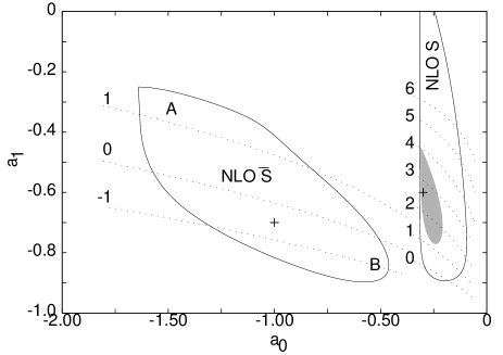
In Fig 4 we have shown the variation of
| (24) |
when one of the parameters in is varied for fixed values of all the other parameters in the set. The minimum of these curves fixes the best-fit value of the parameter, and the points where give the 68.3% confidence limits on this parameter. Uncertainties in the gluon density are shown in greater detail in Figure 5. This shows contour lines of , which encloses the area with 68.3% probability of giving a good description of the data. Also shown in the figure are lines of constant . Although contours give negative values of , we note that contours include positive values as well. Note that our error bars are deliberately conservative, due to our neglect of systematic errors. Since systematic errors are as large as the statistical errors, the naive procedure of summing them in quadrature would have led us to believe that at NLO positive is allowed at .
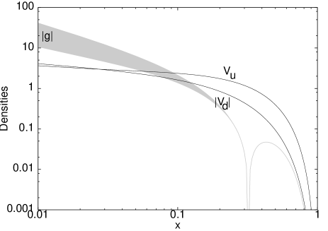
The huge uncertainties in the gluon distribution due to these parameter variations are illustrated in Figure 6. At the polarised gluon density at NLO can lie anywhere in the range from to . This uncertainty at low- prevents us from investigating this theoretically interesting region. The situation is worse at LO where is at the limit of integrability, since . Thus is essentially undetermined.
This large uncertainty in comes because the only constraint on gluon densities at present are the data on variations of . Furthermore, the data at are most effective in constraining , and in this range, the data have large errors. We have quantified this in Figure 7, where we show selected data on in different bins of as a function of (the normalisation has been made arbitrary for ease of viewing). As the bands of variation due to (in the NLO set) show, the data does not constrain the gluon density well.
A few qualitative statements are in order. It is clear that in a scaling theory, DIS data with nucleon or nuclear targets can at most fix two linear combinations of quark densities. However, DIS structure functions are -dependent. Hence, in principle, data of arbitrarily high accuracy fixes these two linear combinations at each — i.e., an infinite number of functions. In QCD there is a more economical description of this dependence involving the set of parton densities given in Section 2. Of course, in the real world data are never infinitely precise, so the question is how accurately does evolution fix these densities. Some part of the answer is clear from Figure 7— improved data at low will constrain much better and , being iso-singlet, would present the best constraint.
We investigated this question quantitatively by generating fake data at from the NLO S set. The values of so generated were smeared randomly over a 10% band to simulate noise in the data, and error bars of 20–30% were assigned to each such data point. This faked set is meant to mimic data that could possibly come from a future polarised HERA experiment. We redid our fits with this faked data set replacing all data on for . This data brings down the error bars in the parameter appearing in by a factor of 4, and improves the errors in by a factor of 2–3. The error estimates obtained with the fake data set are shown in Figure 8. The region of parameter space allowed by this fake data is shown as the grey patch in Figure 5. Taking data at or over a larger range of , both of which would be feasible at polarised HERA, would constrain even better [34]. The ability of RHIC to fix the gluon densities is, of course, well appreciated. However, if DIS experiments can fix the gluon densities better, then polarised RHIC can be used as a discovery machine.
V Applications
A Flavour asymmetry
Unlike previous fits of parton densities which had built in the constraint [7], we have allowed for sea quark densities that violate flavour symmetry. The fits show that the data tolerate, and even prefer, strong flavour symmetry violations. This is easily seen in the first moments of various densities (Table VI). Since and are small, it is clear that the pattern and must follow whenever is large.
It has been suggested [35] that flavour asymmetry in the sea be observed through two combinations of cross sections for production of in longitudinally polarised pp scattering—
| (25) |
where () is defined with the upper (lower) signs. At LO these asymmetries can be written as the ratio of certain combinations of polarised and unpolarised parton densities. At LO the asymmetry for Drell-Yan pairs can also be written in terms of the parton densities. At zero rapidity, is a function of , where is the mass of the pairs and is the center of mass energy of the colliding protons. For production at zero rapidity, the parton densities have to be evaluated at , and hence .
In Figure 9 we have shown these asymmetries at zero rapidity as a function of , or equivalently of . It is clear that at appropriate to RHIC, the iso-triplet spin asymmetry, , is best suited to distinguish the LO S densities from LO . Experimentally studying the dependence of on over even a limited range below GeV would be very useful. is the least suitable measurement for making this distinction.
We have already pointed out that the LO fit is unable to decide on the sign of , and that the NLO fits yield a negative , although positive values are not ruled out. Although previous fits have seen overlapping ranges of allowed , the theoretical bias has been to take large and positive values of . This sign can be easily fixed by various experiments at RHIC or in charm production measurements at HERA [36] or the COMPASS experiment in CERN [37].
We would like to caution that parton densities are renormalisation scheme dependent (and hence unphysical). They are universally applicable to all experiments, as long as each experiment is treated in the same scheme [38]. Our determination of these densities are in the scheme, and statements about their moments are therefore also restricted to this scheme. When interpreting the moments of unphysical parton densities, their scheme dependence must be held in mind.
B Structure functions and couplings
It is possible to construct physical quantities out of the unphysical first moments of the parton densities. For the first moments of the structure functions as given in eq. (14), we obtain the values—
| (26) | |||||
| (27) |
at GeV2. These values are within of each other and they compare well with values deduced from experiments [1, 23, 25].
We can also use eq. (13) to extract the value of . Using as input the above values of derived from our fits and the PDG value for , we find
| (28) |
Since is a physical quantity, it is only to be expected that our determination of should agree with other analyses, such as [9], even if they use some other scheme to arrive at the same result. We will, of course, disagree with them on any scheme dependent quantity, such as . Our maximally flavour symmetry violating fits give physically reasonable results.
C The structure function
Wandzura and Wilczek [39] have derived a sum rule relating the twist-2 part of to —
| (29) |
An additional twist-2 contribution to , suppressed by the ratio of the quark to the nucleon mass [40], is ignored here. Predictions for the twist-3 contribution have been made using bag models [41], QCD sum rules [42] as well as from non-perturbative lattice QCD computations [43]. Since some computations predict large twist-3 contributions to moments of , it becomes interesting to check whether the data on allows such contributions.
Figure 10 shows our “prediction” for the twist-2 part of and compares it to measurements of this structure function. Clearly the data is compatible with the NLO twist-2 prediction (and also with the parton model result, ). Between the prediction and the data, there is little room for a twist-3 contribution. Statistics have to be improved vastly in order to study higher-twist effects. In fact, COMPASS hopes to make this measurement [37].
Since the statistical errors are smallest for , it seems that this is the best candidate in which to look for twist-3 effects. However the data quality needs improvement even here. There is considerable scaling violation in the twist-2 part of , but the large errors prevent any analysis of the -dependence.
D The valence densities
Recently the HERMES collaboration has used semi-inclusive polarised DIS data to extract valence and sea quark densities [33]. We have not used these in our fits because this analysis is performed with parton model formalæ. Nevertheless, it is interesting to compare our fits with these numbers. We display this comparison in Figure 11. The rough agreement is heartening, but the small systematic differences between the fit results and the HERMES extraction of the valence densities shows the need for a more accurate QCD analysis of the experimental data, taking into account properly the dependence through NLO evolution.
E Axion-matter coupling
We present an example of the application of polarised proton scattering to physics beyond the standard model. The Peccei-Quinn solution to the strong CP problem postulates a global symmetry whose spontaneous breakdown generates a (nearly) massless pseudo-Goldstone boson called the axion [44]. There is a variant of the original model which is still viable [45]. The axion, , whose decay constant is , couples to fermions, , of mass by the term
| (30) |
The coupling . The effective Peccei-Quinn charge, , appears in the coupling instead of the actual charge . Here, is given by . There have been several studies [46] of the effective Peccei-Quinn charge of the proton. For three flavours, the LO expression can be written as
| (31) |
where with [47]. for quarks and leptons is highly model dependent. In the so-called KSVZ [48], and other hadronic axion models, . Using quark mass ratios and , obtained by chiral perturbation theory [49], and our LO fits, we find that
| (32) |
The statistical errors in this coupling are dominated by the errors in the fits to polarised parton densities. The uncertainty in the quark masses give smaller contributions to these errors. However, the real source of uncertainty comes from higher loop corrections. An estimate of this theoretical uncertainty can be obtained by inserting the NLO results for various moments into eq. (31). This changes by 25% and by 100%.
The chiral couplings of neutralinos and charginos in generic supersymmetric extensions of the standard model also give rise to effective couplings with matter which depend on the moments of the parton densities. Such couplings are often needed in astrophysical contexts. Unless these couplings are examined to 2-loop order, they should not be evaluated with the NLO moments.
VI Conclusions
We have made global QCD analyses of data on the asymmetry from polarised DIS without making overly restrictive assumptions about the flavour content of the sea. We have extracted polarised parton densities which can be used with the CTEQ4 set of unpolarised densities. Our NLO analyses (in the scheme) yield the parameter sets given in Tables II and III, and the LO analyses give the sets displayed in Tables IV and V. Strong flavour symmetry violation in the sea is supported by the sets of densities in which the first moment of the singlet sea quark density is much smaller than that of the triplet sea quark density. We also found in the NLO fits that the first moment of the gluon density is preferentially negative, although positive values are within 2–3 of the best fits. The LO fits, to the contrary, prefer a positive sign for , although negative values are allowed within 2–3 of the central values. All physical quantities obtained from the first moments of our fitted densities have completely sensible values, as they must have.
We have shown that the polarised HERA option may yield highly accurate measurements of the polarised gluon densities if measurements of in the range can be performed with errors of about 25%. Measurements of the asymmetry in the iso-triplet part of production at RHIC are likely to be able to pin down the flavour content of the sea. Measurements at future facilities for spin physics thus nicely complement each other.
We have checked that our parametrisations are roughly consistent with semi-inclusive DIS data, although a full QCD analysis of this data remains to be performed. We have also shown that these parametrisations, when used to determine the twist-2 part of leave very little room for a twist-3 part to this structure function. Finally, we have determined the coupling of hadronic axions to matter— an input into several astrophysical constraints on the invisible axion.
In a future publication we plan to make a more detailed study of several issues, including the proper inclusion of systematic experimental errors into the analysis and several other technical issues concerning NLO QCD global fits.
We would like to thank Willy van Neerven for several discussions and clarifications. We also thank the organisers of the 6th Workshop on High Energy Physics Phenomenology (WHEPP-6), Chennai, January 2000, where a portion of this work was completed.
REFERENCES
-
[1]
M. J. Alguard et al. (E80), Phys. Rev. Lett. 37 (1976) 1261;
G. Baum et al. (E130), Phys. Rev. Lett. 51 (1983) 1135;
J. Ashman et al. (EMC), Phys. Lett. B 206 (1988) 364. -
[2]
J. Ellis and R. Jaffe, Phys. Rev., D 9 (1974) 1444;
Erratum— ibid., D 10 (1974) 1669;
M. Gourdin, Nucl. Phys., B 38 (1972) 418. - [3] J. D. Bjorken, Phys. Rev., 148 (1966) 1467,
-
[4]
S. A. Larin and J. A. M. Vermaseeren, Phys. Lett., B 259 (1991) 345;
S. A. Larin, Phys. Lett., B 334 (1994) 192. - [5] G. Altarelli et al., Nucl. Phys., B 496 (1997) 337.
-
[6]
R. Mertig and W. van Neerven, Z. Phys., C 70 (1996) 637;
W. Vogelsang, Phys. Rev., D 54 (1996) 2023. -
[7]
M. Glück et al., Phys. Rev. D 53 (1996) 4775;
T. Gehrmann and W. J. Stirling, Phys. Rev., D 53 (1996) 6100;
K. Abe et al. (E-154), Phys. Lett. B 405 (1997) 180;
C. Bourrely et al., Prog. Theor. Phys. 99 (1998) 1017;
G. Altarelli et al., Acta Phys. Polon. B 29 (1998) 145;
D. de Florian, O. Sampayo and R. Sassot, Phys. Rev., D 57 (1998) 5803;
L. E. Gordon, M. Goshtasbpour and G. P. Ramsey, Phys. Rev. D 58 (1998) 094017;
E. Leader, A. V. Sidorov and D. B. Stamenov, Phys. Rev. D 58 (1998) 114028;
Y. Goto et al., e-print hep-ph/0001046. - [8] H. L. Lai et al., Phys. Rev., D 55 (1997) 1280.
- [9] R. D. Ball, S. Forte and G. Ridolfi, Phys. Lett. B 378 (1996) 255.
- [10] E. Leader, A. V. Sidorov and D. B. Stamenov, Phys. Lett. B 445 (1998) 232.
-
[11]
W. J. Marciano, Phys. Rev., D 29 (1984) 580;
J. F. Owens and W.-K. Tung, Ann. Rev. Nucl. Part. Sci., 42 (1992) 291. -
[12]
F. E. Close and D. Sivers, Phys. Rev. Lett. 39 (1977) 1116;
S. J. Brodsky and I. Schmidt, Phys. Lett. B 234 (1990) 114. - [13] R. L. Jaffe, Phys. Lett., B 193 (1987) 101.
- [14] L. H. Ahrens et al., Phys. Rev. D 35 (1987) 785.
-
[15]
M. Fukugita et al. Phys. Rev. Lett. 75 (1995) 2092;
S. J. Dong et al. Phys. Rev. Lett. 75 (1995) 2096. -
[16]
S. Gupta, M. V. N. Murthy and J. Pasupathy, Phys. Rev. D 39 (1989) 2547;
E. M. Henley, W. Y. P. Hwang and L. S. Kisslinger, Phys. Rev. D 46 (1992) 431. -
[17]
C. Caso et al., Euro. Phys. J. C 3 (1998) 1;
The Particle Data Group, http://pdg.lbl.gov, June 1999. -
[18]
D. B. Kaplan and A. Manohar, Nucl. Phys. B 310 (1988) 527;
H. J. Lipkin, Phys. Lett. B 230 (1988) 135;
M. Anselmino, B. L. Ioffe and E. Leader, Sov. J. Nucl. Phys. 49 (1989) 136;
E. Leader and D. B. Stamenov, e-print hep-ph/9912345. - [19] G. Altarelli, S. Forte and G. Ridolfi, Nucl. Phys., B 534 (1998) 277.
- [20] W. H. Press et al., Numerical Recipes in Fortran, Cambridge University Press, 1990.
- [21] B. Adeva et al. (SMC), Phys. Rev. D 58 (1998) 112001.
- [22] K. Abe et al. (E143), Phys. Rev. D 58 (1998) 112003.
- [23] K. Abe et al. (E154), Phys. Rev. Lett. 79 (1997) 26.
- [24] A. Airapetian et al. (HERMES), Phys. Lett. B 442 (1998) 484.
- [25] P. L. Anthony et al. (E142), Phys. Rev. D 54 (1996) 6620.
-
[26]
B. Desplanques, Phys. Lett B 203 (1988) 200;
A. W. Thomas and W. Melnitchouk, Nucl. Phys. A 631 (1998) 296c. -
[27]
R. M. Woloshyn, Nucl. Phys. A 496 (1988) 749;
S. Scopetta et al., Phys. Lett. B 404 (1997) 223. -
[28]
M. Anselmino, A. Efremov and E. Leader, Phys. Rep. 261 (1995) 1;
B. Lampe and E. Reya, e-print hep-ph/9810270. -
[29]
D. Adams et al. (SMC), Phys. Rev. D 56 (1997) 5330;
K. Abe et al. (E143), Phys. Rev. D 58 (1998) 112003. -
[30]
D. Adams et al. (SMC), Phys. Lett. B 396 (1997) 338;
K. Abe et al. (E143), Phys. Rev. D 58 (1998) 112003;
P. L. Anthony et al. (E155), Phys. Lett. B 463 (1999) 339. -
[31]
K. Abe et al. (E143), Phys. Rev. D 58 (1998) 112003
K. Abe et al. (E154), Phys. Lett. B 404 (1997) 377. - [32] B. Adeva et al. (SMC), Phys. Lett. B 420 (1998) 180.
- [33] K. Ackerstaff et al. (HERMES), Phys. Lett. B 464 (1999) 123.
- [34] A. De Roeck et al., Eur. Phys. J. C 6 (1999) 121.
-
[35]
M. A. Doncheski et al., Phys. Rev. D 49 (1994) 3261;
H.-Y. Cheng, M.-L. Huang and C. F. Wai, Phys. Rev. D 49 (1994) 1272. -
[36]
T. Gehrmann, e-print hep-ph/9908500;
J. Feltesse and A. Schäfer, Proceedings of the workshop, “Future Physics at HERA”, Hamburg, 1995/96, Eds. G. Ingelman, A. De Roeck, and R. Klanner, DESY (Hamburg, 1996). - [37] L. Schmitt (for the Compass Collaboration), Contribution at the International Conference on High Energy Physics, ICHEP, Vancouver, 1998.
- [38] A. Manohar, Phys. Rev. Lett. 66 (1991) 289.
- [39] S. Wandzura and F. Wilczek, Phys. Lett. B 72 (1977) 195.
- [40] X. Song, Phys. Rev. D 54 (1996) 1955.
-
[41]
M. Stratmann, Z. Phys. C 60 (1993) 763;
R. L. Jaffe and X. Ji, Phys. Rev. D 43 (1991) 724;
see also [40]. -
[42]
I. I. Balitsky, V. M. Braun, and A. V. Kolesnichenko,
Phys. Lett. B 242 (1990) 245;
E. Stein et al., Phys. Lett. B 343 (1995) 369. - [43] M. Göckeler et al., Phys. Rev. D 53 (1996) 2317.
- [44] R. D. Peccei and H. Quinn, Phys. Rev. Lett. 38 (1977) 1440.
- [45] M. Dine, W. Fischler and M. Srednicki, Phys. Lett. B 104 (1981) 199.
-
[46]
D. B. Kaplan, Nucl. Phys. B 260 (1985) 215;
M. Srednicki, Nucl. Phys. B 260 (1985) 689;
R. Mayle,et al., Phys. Lett. B 203 (1988) 188. - [47] G. Raffelt, Phys. Rep. 198 (1990) 1.
-
[48]
J. E. Kim, Phys. Rev. Lett. 43 (1979) 103;
M. A. Shifman, A. I. Vainshtein and V. I. Zakharov, Nucl. Phys. B 166 (1980) 493. - [49] J. Gasser and H. Leutwyler, Phys. Rep. 87 (1982) 77.
| Experiment | Points | LO S | LO | NLO S | NLO |
|---|---|---|---|---|---|
| SMC (p) | 48 | 46.6 | 48.4 | 43.4 | 42.1 |
| SMC (d) | 53 | 53.5 | 53.7 | 54.3 | 50.0 |
| E-143 (p) | 43 | 48.2 | 47.8 | 48.7 | 50.2 |
| E-143 (d) | 43 | 62.1 | 60.3 | 61.0 | 57.0 |
| HERMES (p) | 9 | 23.8 | 18.8 | 12.6 | 15.1 |
| HERMES (n) | 4 | 1.7 | 1.6 | 1.5 | 1.7 |
| E-142 (n) | 15 | 15.9 | 16.8 | 18.7 | 21.1 |
| E-154 (n) | 8 | 22.9 | 16.7 | 3.3 | 2.3 |
| Total | 224 | 274.6 | 264.0 | 243.7 | 239.4 |
| density | |||||
|---|---|---|---|---|---|
| () | 12.2 () | ||||
| () | 2.2 () | ||||
| 0.009 () | 8 () | ||||
| 7 () | |||||
| density | |||||
|---|---|---|---|---|---|
| 1.74 () | |||||
| 1.6 () | |||||
| () | () | 6.5 () | |||
| density | |||||
|---|---|---|---|---|---|
| () | |||||
| density | |||||
|---|---|---|---|---|---|
| 1.91 () | () | ||||
| () | |||||
| LO S | LO | NLO S | NLO | |
|---|---|---|---|---|
| 0.875 () | 0.829 () | 0.909 () | 0.85 () | |
| () | () | () | () | |
| () | () | () | () | |
| - | - | |||
| - | 0.107 () | - | () | |
| () | 0.0212 () | () | () | |
| () | () | () | 0.024 () | |
| () | () | () | () |