CERN-TH/99-415

hep-ph/0001286

January 2000

Top–Antitop Pair Production close to Threshold:
Synopsis of recent NNLO Results

A. H. Hoang^a, M. Beneke^a,b, K. Melnikov^c, T. Nagano^d, A. Ota^d, A. A. Penin^e, A. A. Pivovarov^f, A. Signer^g, V. A. Smirnov^h, Y. Sumino^d, T. Teubner^b, O. Yakovlevⁱ, A. Yelkhovsky^j

^a Theory Division, CERN, CH-1211 Geneva 23, Switzerland
^b Institut für Theoretische Physik E, RWTH Aachen, D-52056 Aachen, Germany
^c Stanford Linear Accelerator Center, Stanford University, Stanford CA 94309, USA
^d Department of Physics, Tohoku University, Sendai, 980-8578 Japan
^e Institute for Theoretical Physics, University Hamburg, D-22761 Hamburg, Germany
^f Institute for Nuclear Research of the Russian Academy of Sciences, Moscow 117312, Russia
^g Department of Physics, University of Durham, Durham DH1 3LE, England
^h Nuclear Physics Institute, Moscow State University, 119889 Moscow, Russia
ⁱ Randall Laboratory of Physics, University of Michigan, Ann Arbor, Michigan 48109-1120, USA
^j Budker Institute for Nuclear Physics, 630090 Novosibirsk, Russia

Abstract

Using non-relativistic effective theories, new next-to-next-to-leading order (NNLO) QCD corrections to the total $t\bar{t}$ production cross section at the Linear Collider have been calculated recently. In this article the NNLO calculations of several groups are compared and the remaining uncertainties are discussed. The theoretical prospects for an accurate determination of top quark mass parameters are discussed in detail. An outlook on possible future improvements is given.

1 Introduction

Top–antitop quark pair production close to the threshold will provide an integral part of the top quark physics program at the Linear Collider (LC). The theoretical interest in the top–antitop quark threshold arises from the fact that the large top quark mass and width ($\Gamma_{t}\approx 1.5$ GeV) lead to a suppression of non-perturbative effects [1, 2, 3]. This makes perturbative methods a reliable tool to describe the physics of non-relativistic $t\bar{t}$ pairs, and allows for measurements of top quark properties directly at the parton level. Due to the large top width the total $t\bar{t}$ production cross section line shape is a smooth function of the energy, which rises rapidly at the point where the remnant of a toponium 1S resonance can be formed. From the energy where this increase occurs, the top quark mass can be determined, whereas shape and height of the cross section near threshold can be used to determine $\Gamma_{t}$, the coupling strength of top quarks to gluons and, if the Higgs boson is not heavy, the top Yukawa coupling [4]. From differential quantities, such as the top momentum distribution [5, 6], the forward–backward asymmetry or certain leptonic distributions [7, 8], one can obtain measurements of $\Gamma_{t}$, the top quark spin and possible anomalous couplings.

The measurements of the top quark mass and the total top quark width from a threshold line shape scan are particularly interesting. In contrast to the standard top mass determination method, which relies on the reconstruction of the invariant mass of jets originating from a single top quark, the line shape measurement has the advantage that only colour-singlet $t\bar{t}$ events have to be counted. Therefore, the effects of final state interactions are suppressed, and systematic uncertainties in the top mass determination are small. For the total top quark width only a few other ways to determine it directly are known. Simulation studies, which also took into account the smearing of the c.m. energy from beam effects, have shown that, for a total luminosity of 100 fb^-1, statistical and systematical experimental uncertainties in the top mass determination are below 50 MeV [9]. The top quark width can be determined with experimental uncertainties of better than 20% for given top quark mass and $\alpha_{s}$ [10, 11, 12].

With this prospect in view it is obvious that a careful analysis and assessment of theoretical uncertainties in the prediction of the total cross section is mandatory, in order to determine whether the theoretical precision can meet the experimental one. Within the last two years, considerable progress has been achieved in higher order calculations of the total cross section. Using the concept of effective field theories, calculations of NNLO QCD corrections to the total cross section have been carried out by several groups: Hoang–Teubner [13, 14], Melnikov–Yelkhovsky [15], Yakovlev [16], Beneke–Signer–Smirnov [17], Nagano–Ota–Sumino [18] and Penin–Pivovarov [19]. In contrast to previous LO [20] and NLO calculations [4, 5, 6, 7, 8, 21], the new results at NNLO do not rely on potential models that need phenomenological input, but represent first-principle QCD calculations. The results are not just some new higher order corrections, but have led to a number of surprising and important insights. The NNLO corrections to the location where the cross section rises and the height of the cross section were found to be much larger than expected from the known NLO calculations. It was suggested that the large corrections to the location of the rise are an artifact of the on-shell (pole) mass renormalisation [22]. Several authors realized that the quark pole mass cannot be extracted with an uncertainty smaller than ${\cal{O}}(\Lambda_{\rm QCD})$ from non-relativistic heavy quark–antiquark systems [23, 22, 24]. New top quark mass definitions were subsequently employed to allow for a stable extraction of the top quark mass parameter [17, 14]. The remaining uncertainties in the normalisation of the cross section seem to jeopardise the measurements of the top width, the top quark coupling to gluons, and the Higgs boson. The results obtained by all groups are formally equivalent at the NNLO level. However, they differ in the use of the calculational methods and the intermediate regularization prescriptions, and their treatments of higher order corrections. Apart from analysing the theoretical uncertainties estimated from the result of one individual group, a comparison of the results obtained from the different groups serves as an additional useful instrument to assess the theoretical uncertainties. In this article the results for the NNLO QCD calculations for the total cross section obtained by the individual groups are compared and an overview of what has been achieved so far based on the results of all groups is given. As an outline for possible future work, some remaining open questions are addressed.

The outline of this note is as follows: in Sec. 2 a brief introduction into the technical issues relevant to the calculation of the total cross section at NNLO is given, and some aspects of the effective field theory approach are reviewed. In Sec. 3 the NNLO QCD calculations obtained by the different groups are compared in the pole mass scheme. In Sec. 4 three alternative mass definitions tested by Beneke–Signer–Smirnov, Hoang–Teubner and Melnikov–Yelkhovsky are discussed. Section 5 contains a brief summary and mentions some issues that should be addressed in the future.

2 Total Cross Section at NNLO and Effective Theory Approach

For the total cross section close to the threshold, where the velocity $v$ of the top quarks is small, $v\ll 1$, the conventional perturbative expansion in the strong coupling breaks down, owing to singular terms $\sim(\alpha_{s}/v)^{n}$ that arise in the $n$-loop amplitude. This singularity is caused by the instantaneous Coulomb attraction between the top quarks, which cannot be treated as a perturbation if their relative velocity is small. It is therefore mandatory to resum the terms that are singular in $v$ to all orders in $\alpha_{s}$. At LO in the non-relativistic expansion of the total cross section, this amounts to resumming all terms proportional to $v(\alpha_{s}/v)^{n}$, $n=0,\ldots,\infty$. The most convenient tool to carry out this resummation is the Schrödinger equation

$$\bigg{(}\,-\frac{\vec{\nabla}^{2}}{M_{t}^{\rm pole}}-\frac{C_{F}\,\alpha_{s}}{|\mbox{\boldmath$r$}|}-(\sqrt{q^{2}}-2M_{t}^{\rm pole})-i\Gamma_{t}\,\bigg{)}\,G(\mbox{\boldmath$r$},\mbox{\boldmath$r$}^{\prime},\sqrt{q^{2}}) = \delta^{(3)}(\mbox{\boldmath$r$}-\mbox{\boldmath$r$}^{\prime})\,,$$ (1)

where $M_{t}^{\rm pole}$ and $\Gamma_{t}$ are the top quark pole mass and width, respectively. The Schrödinger equation has the simple form shown in Eq. (1) only in the pole mass scheme. The decay of the top quark is implemented by adding the term $i\,\Gamma_{t}$ to the c.m. energy $\sqrt{q^{2}}$ [3]. At LO in the non-relativistic expansion, counting $\Gamma_{t}$ as being of order $M_{t}^{\rm pole}\alpha_{s}^{2}$, this is the correct way to implement electroweak effects [17, 14]. The total cross section $\sigma_{\rm tot}(e^{+}e^{-}\to\gamma^{*},Z^{*}\to t\bar{t})$ reads

$$\sigma_{\rm tot}^{\gamma,Z}(q^{2}) = \sigma_{pt}\,\bigg{[}\,Q_{t}^{2}-2\,\frac{q^{2}}{q^{2}-M_{Z}^{2}}\,v_{e}\,v_{t}\,Q_{t}+\bigg{(}\frac{q^{2}}{q^{2}-M_{Z}^{2}}\bigg{)}^{2}\,\Big{[}v_{e}^{2}+a_{e}^{2}\Big{]}\,v_{t}^{2}\,\bigg{]}\,R^{v}(q^{2})$$ (2)

$$+\,\sigma_{pt}\,\bigg{(}\frac{q^{2}}{q^{2}-M_{Z}^{2}}\bigg{)}^{2}\,\Big{[}v_{e}^{2}+a_{e}^{2}\Big{]}\,a_{t}^{2}\,R^{a}(q^{2})\,,$$

where

$$\sigma_{pt} = \frac{4\,\pi\,\alpha^{2}}{3\,q^{2}}\,,$$ (3)

$$v_{f} = \frac{T_{3}^{f}-2\,Q_{f}\,\sin^{2}\theta_{W}}{2\,\sin\theta_{W}\,\cos\theta_{W}}\,,$$ (4)

$$a_{f} = \frac{T_{3}^{f}}{2\,\sin\theta_{W}\,\cos\theta_{W}}\,.$$ (5)

Here, $\alpha$ is the fine structure constant, $Q_{t}=2/3$ the electric charge of the top quark, $\theta_{W}$ the Weinberg angle, and $T_{3}^{f}$ refers to the third component of the weak isospin; $R^{v}$ and $R^{a}$ represent the contributions to the cross section induced by vector- and axial-vector current, respectively. $R\equiv Q_{t}^{2}R^{v}$ is equal to the total normalised photon-induced cross section, which is usually referred to as the $R$-ratio. Close to threshold, $\sigma_{\rm tot}^{\gamma,Z}$ is dominated by the vector-current contribution $R^{v}$, which describes top quark pairs in an angular momentum S-wave state. Higher angular momentum states are suppressed by additional powers of $v$; P-wave production, which is associated to the axial-vector current contribution $R^{a}$ is suppressed by $v^{2}$ and needs to be taken into account at NNLO [25, 19, 14, 26]. The absorptive part of $G(\mbox{\boldmath$0$},\mbox{\boldmath$0$},\sqrt{q^{2}})$, obtained from Eq. (1), is the first term of a non-relativistic expansion of $R^{v}$ close to threshold:

$$R^{v}(q^{2}\approx 4M_{t}^{2}) = \frac{72\,\pi}{q^{2}}\,{\mbox{Im}}\Big{[}G(\mbox{\boldmath$0$},\mbox{\boldmath$0$},\sqrt{q^{2}})\Big{]}+\ldots\,.$$ (6)

To determine NLO corrections to the cross section, corresponding to a resummation of all terms $\propto v(\alpha_{s}/v)^{n}\times[\alpha_{s},v]$, $n=0,\ldots,\infty$, the one-loop corrections to the Coulomb potential [27] have to be added in Eq. (1) and a short-distance correction to the top–antitop production current has to be included [28]. The latter is implemented by multiplying the Green function of the Schrödinger equation by a factor $C=1+c_{1}\frac{\alpha_{s}}{\pi}$, where $c_{1}$ is a real number. The NLO corrections do not pose any conceptual problem, because the short-distance corrections to $C$ factorise unambiguously, and because the absorptive part of the Green function does not contain any ultraviolet divergences at this order. The corrections at NNLO, corresponding to a resummation of all terms $\propto v(\alpha_{s}/v)^{n}\times[\alpha_{s}^{2},\alpha_{s}\,v,v^{2}]$, $n=0,\ldots,\infty$, require the inclusion of the kinetic energy term $-\frac{\vec{\nabla}^{4}}{4\,M_{t}^{3}}$, two-loop corrections to the static potential [29] and new potentials suppressed by additional powers of $1/M_{t}^{2}$ and $\alpha_{s}/M_{t}$ into Eq. (1). In addition, the short-distance factor $C$ has to be determined at the two-loop level [30, 31]. The new potentials are the generalisation of the Breit–Fermi potential, known from positronium, in QCD. The determination of the NNLO corrections is non-trivial because the additional mass-suppressed terms in the Schrödinger equation lead to UV divergences in the absorptive part of the Green function $G$. This is because they contain momenta to a high positive power. These divergences are a consequence of the non-relativistic expansion.

The problem of UV divergences can be conveniently dealt with in the framework of non-relativistic effective theories. All the NNLO calculations performed in Refs. [13, 15, 16, 17, 18, 19, 14] have been carried out in this framework. In the effective field theory approach the top quark and the gluonic degrees of freedom that are off-shell in the non-relativistic top–antitop-quark system are integrated out, leaving only those degrees of freedom as dynamical that can become on-shell. The relevant momentum regimes associated with non-relativistic degrees of freedom have a non-trivial structure [32] and were finally identified by Beneke and Smirnov [30]. The resulting effective field theory obtained by integrating out the degrees of freedom that are off-shell has been called “potential non-relativistic QCD” (PNRQCD) [33]. PNRQCD represents an effective theory of NRQCD; the latter was first proposed by Caswell and Lepage [34] and is widely used in charmonium and bottomonium physics [35]. As the NRQCD Lagrangian, the PNRQCD Lagrangian contains an infinite number of operators, where operators of higher dimension are associated to interactions suppressed by higher powers in $v$. The corresponding Wilson coefficients can be determined perturbatively (as a conventional series in $\alpha_{s}$) by matching on-shell scattering amplitudes in PNRQCD and full QCD. The main feature of PNRQCD is the existence of spatially non-local instantaneous four-quark interactions, which represent an instantaneous interaction of a quark–antiquark pair separated by some spatial distance $r$:

$${\cal{L}}^{\mbox{\tiny PNRQCD}}_{\tiny\rm non-local} = \int d^{3}\mbox{\boldmath$r$}\Big{(}\psi^{\dagger}\psi\Big{)}(\mbox{\boldmath$r$})\,V(\mbox{\boldmath$r$})\,\Big{(}\chi^{\dagger}\chi\Big{)}(0)\,.$$ (7)

Here, $\psi$ and $\chi$ represent the two-component Pauli spinors describing the top and antitop quarks after the corresponding small component has been integrated out. The Wilson coefficients $V(\mbox{\boldmath$r$})$ of these non-local interactions are generalisations of the concept of the heavy quark potential. We emphasise that these Wilson coefficients are strict short-distance quantities that can be calculated perturbatively. In addition, PNRQCD contains the interactions of dynamical gluons (having energies and momenta of the order of the top quark kinetic energy) with the top quarks. These dynamical gluons lead to top–antitop quark interactions that are not only non-local in space but also in time. These interactions are called “retardation effects”. External electroweak currents, which describe production and annihilation of a top quark pair are rewritten in terms of PNRQCD currents, providing a systematic small-velocity-expansion of the corresponding relativistic current–current correlators. The Wilson coefficients of the PNRQCD currents contain short-distance information specific to the corresponding electroweak current producing or annihilating the top–antitop-quark pair. The short-distance factor $C$ is the modulus square of the Wilson coefficient of the first term in the non-relativistic expansion of the vector current. PNRQCD provides so-called “velocity counting rules” that unambiguously state which of the operators have to be taken into account to describe the quark–antiquark dynamics at a certain parametric precision. For the description of a non-relativistic $t\bar{t}$ pair at NNLO, these rules show that the interactions of dynamical gluons can be neglected. The resulting equation of motion for a heavy quark–antiquark pair has the form of Eq. (1), supplemented by corrections up to NNLO. UV divergences in the calculation of the absorptive part of the Green function are subtracted and interpreted in the context of a particular regularization scheme for PNRQCD. The absorptive part of the Green function then contains a dependence on the regularization scheme parameter. This dependence on the regularization parameter is cancelled by that of the two-loop corrections to the short-distance factor $C$.

We note that, strictly speaking, the new NNLO calculations represent true NNLO results only for the case of a stable top quark. None of the new NNLO calculations contains a consistent treatment of electroweak effects at NNLO. All groups took into account the top quark width by adding $i\,\Gamma_{t}$ to the c.m. energy in the Schrödinger equation, as shown in Eq. (1). However, we do not expect that the neglected electroweak corrections will exceed several per cent for the total cross section.

3 NNLO Results for the Total Cross Section
in the Pole Mass Scheme

Six groups have calculated the NNLO QCD corrections to the total cross section close to threshold: Hoang–Teubner [13, 14], Melnikov–Yelkhovsky [15], Yakovlev [16], Beneke–Signer–Smirnov [17], Nagano–Ota–Sumino [18] and Penin–Pivovarov [19]. In this section the methods of the different groups are briefly summarised and differences are pointed out. The results are compared numerically in the pole mass scheme. Because NNLO corrections are only relevant to the vector-current-induced total production cross section, we will only compare the normalised photon-induced cross section $R$. Results for the cross section including also the full Z-exchange contributions can be found in Refs. [26, 19, 14]. The methods for the NNLO results from the groups Melnikov–Yelkhovsky, Yakovlev and Nagano–Ota–Sumino are identical. Because the numerical results provided by these groups for this comparison agree with each other to better than one per mille, they will be treated as belonging to a single group.

The different groups have used the following methods in their NNLO calculations:

• Hoang–Teubner (HT) [14] have solved the NNLO Schrödinger equation exactly in momentum space representation. As ultraviolet regularization they restricted all momenta to be smaller than the cutoff $\Lambda$, which is of the order of the top quark mass. The short-distance coefficient $C$ was determined by using the “direct matching procedure” [36], where the total cross section in the effective field theory is matched to the total cross section in QCD in the limit $\alpha_{s}\ll v\ll 1$ and for $\Gamma_{t}=0$. The result for the total cross section depends on two scales, $\mu_{\rm soft}$, the renormalisation scale of the strong coupling in the static potential and the cutoff scale $\Lambda$. The renormalisation scale in the short-distance coefficient $C$ is also $\mu_{\rm soft}$. The sensitivity to $\Lambda$ is considerable at LO and has been shown to be small at NLO and NNLO.

• Melnikov–Yelkhovsky–Yakovlev–Nagano–Ota–Sumino (MYYNOS) [15, 16, 18] solved the NNLO Schrödinger equation exactly in coordinate space representation. As regularization prescription they determined the Green function at a finite distance $r_{0}$ from the origin and expanded in $r_{0}$. Only logarithms of $r_{0}$ were kept and inverse powers of $r_{0}$ were discarded. The value of $r_{0}$ was chosen of the order of the inverse top quark mass. The short-distance coefficient $C$ was determined by using the “direct matching procedure”. The result for the total cross section depends on three scales, $\mu_{\rm soft}$, the renormalisation scale in the static potential, $1/r_{0}$, the cutoff scale, and $\mu_{\rm hard}$, the renormalisation scale in the short-distance coefficient $C$. The scale $\mu_{\rm hard}$ was set equal to the top quark mass. The sensitivity to $r_{0}$ has been shown to be small.

• Penin–Pivovarov (PP) [19] solved the Schrödinger equation perturbatively in coordinate space representation. They started from the analytically known solution of the LO Coulomb problem and determined NLO and NNLO corrections analytically via Rayleigh-Schrödinger time-independent perturbation theory. As regularization prescription they determined the Green function at a finite distance to the origin, discarding all power-like divergences. In order to avoid multiple poles in the energy denominators of the Green function, which naturally arise in a perturbative determination of the Green function and which lead to instabilities in the cross-section shape, PP supplemented their calculation by reabsorbing the corrections to the energy eigenvalues into single-pole energy denominators. The short-distance coefficient $C$ was determined by using the “direct matching procedure”. The result for the total cross section depends on three scales, $\mu_{\rm soft}$, the renormalisation scale in the static potential, $\mu_{\rm fac}$, the cutoff scale, and $\mu_{\rm hard}$, the renormalisation scale in the short-distance coefficient $C$. The scales $\mu_{\rm fac}$ and $\mu_{\rm hard}$ have been chosen of the order of the top quark mass. The sensitivity to variations of $\mu_{\rm fac}$ and $\mu_{\rm hard}$ has been shown to be small.

• Beneke–Signer–Smirnov (BSS) [17] solved the Schrödinger equation perturbatively using dimensional regularization as a regularization prescription. They started from the analytically known solution of the LO Coulomb problem and determined all corrections analytically via Rayleigh–Schrödinger time-independent perturbation theory. At NLO BSS included the second iteration of the one-loop corrections to the static potential. The short-distance coefficient $C$ was determined by extracting the hard momentum contribution in the two-loop amplitude for $\gamma\to t\bar{t}$ close to threshold for $\Gamma_{t}=0$ [31], using the “threshold expansion” [30], which is an algorithm to calculate the asymptotic expansion of diagrams describing processes involving massive quark–antiquark pairs in the kinematic region close to the two-particle threshold. In order to avoid the destabilising effects of multiple poles in the energy denominators of the Green function, BSS supplemented their result by reabsorbing the corrections to the two lowest lying energy eigenvalues into single-pole energy denominators. In contrast to all other groups, BSS have not implemented the short-distance coefficient $C$ as a global factor, but have expanded $C$ together with the non-relativistic corrections to the Green function up to NNLO. The result of BSS depends on the scale $\mu_{\rm soft}$ and on the QCD/NRQCD matching scale $\mu_{\rm h}$. The dependence on the scale $\mu_{\rm h}$ has been shown to be small.

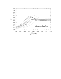
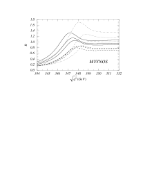
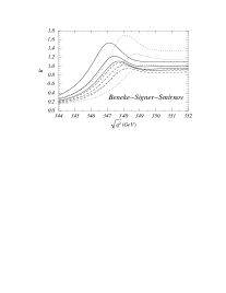
Figure 1: The total normalised photon-induced $t\bar{t}$ cross section $R$ at the LC versus the c.m. energy in the threshold regime at LO (dotted curves), NLO (dashed) and NNLO (solid) in the pole mass scheme for $M_{t}^{\rm pole}=175.05$ GeV, $\alpha_{s}(M_{Z})=0.119$ , $\Gamma_{t}=1.43$ GeV and $\mu_{\rm soft}=15$, $30$, $60$ GeV. The plots have been generated from results provided by the groups Hoang-Teubner (HT), Melnikov-Yelkhovsky-Yakovlev-Nagano-Ota-Sumino (MYYNOS), Penin-Pivovarov (PP) and Beneke-Signer-Smirnov (BSS).

Order	LO			NLO			NNLO
$\mu_{\rm soft}$[GeV]	$15$	$30$	$60$	$15$	$30$	$60$	$15$	$30$	$60$
HT	$1.22$	$0.96$	$0.80$	$0.86$	$0.90$	$0.88$	$1.14$	$1.08$	$1.04$
	$348.06$	$348.69$	$349.26$	$347.75$	$347.93$	$348.17$	$347.12$	$347.34$	$347.55$
MYYNOS	$1.70$	$1.28$	$1.03$	$0.80$	$0.86$	$0.87$	$1.33$	$1.15$	$1.06$
	$348.14$	$348.79$	$349.36$	$347.83$	$348.03$	$348.27$	$347.22$	$347.48$	$347.68$
PP	$1.70$	$1.28$	$1.03$	$0.77$	$0.87$	$0.89$	$1.56$	$1.16$	$1.04$
	$348.14$	$348.79$	$349.36$	$347.96$	$348.04$	$348.29$	$347.12$	$347.46$	$347.71$
BSS	$1.70$	$1.28$	$1.03$	$1.08$	$1.02$	$0.95$	$1.53$	$1.23$	$1.12$
	$348.15$	$348.79$	$349.36$	$347.81$	$348.03$	$348.26$	$347.14$	$347.46$	$347.70$

Table 1: The values of $R$ (upper numbers) at the respective peak position (lower numbers in units of GeV) at LO, NLO and NNLO in the pole mass scheme for $M_{t}^{\rm pole}=175.05$ GeV, $\alpha_{s}(M_{Z})=0.119$, $\Gamma_{t}=1.43$ GeV and $\mu_{\rm soft}=15$, $30$, $60$ GeV. The values have been determined from results provided by the groups Hoang-Teubner (HT), Melnikov–Yelkhovsky–Yakovlev–Nagano–Ota–Sumino (MYYNOS), Penin–Pivovarov (PP) and Beneke–Signer–Smirnov (BSS).

In Figs. 1 the total normalised photon-induced cross section $R$ obtained from HT ($\Lambda=M_{t}^{\rm pole}$), MYYNOS ($r_{0}=e^{2-\gamma}/2M_{t}^{\rm pole}$, $\mu_{\rm hard}=M_{t}^{\rm pole}$), PP ($\mu_{\rm fac}=\mu_{\rm hard}=M_{t}^{\rm pole}$) and BSS ($\mu_{\rm h}=M_{t}^{\rm pole}$) are displayed at LO (dotted lines), NLO (dashed lines) and NNLO (solid lines) in the non-relativistic expansion in the pole mass scheme for $M_{t}^{\rm pole}=175.05$ GeV, $\alpha_{s}(M_{Z})=0.119$, $\Gamma_{t}=1.43$ GeV and $\mu_{\rm soft}=15$, $30$, $60$ GeV. The value for the top quark pole mass is the highest-order entry of Table 3, taking $\overline{m}_{t}(\overline{m}_{t})=165$ GeV as a reference value. The range $15$–$60$ GeV for $\mu_{\rm soft}$ is chosen, because it covers the typical top quark three momentum in the $t\bar{t}$ system. The effects of the beam energy spread due to initial-state radiation and beamstrahlung, which lead to a smearing of the effective centre-of-mass energy and a loss of luminosity, are not included in this comparison. In Table 1 the values of $R$ (upper numbers) at the visible maximum (lower numbers in units of GeV) at LO, NLO and NNLO in the pole mass scheme are displayed using the same set of parameters as in Figs. 1. The various results presented in Figs. 1 and Table 1 are of the same order and only differ with respect to the treatment of higher order corrections, and with respect to the regularization scheme.

As far as the position of the maximum, called “peak position” in the rest of this article, is concerned the results of all groups are consistent: they all show that the position of the peak receives large NNLO corrections and that the peak is moved to smaller c.m. energies at higher orders. For $\mu_{\rm soft}=15/30/60$ GeV, the NLO shift is around $300/800/1200$ MeV versus $600$–$800/600/600$ MeV at NNLO. The convergence is better for higher renormalisation scales, but the size of the overall shift is also increasing. In addition, the dependence of the peak position on the renormalisation scale is not reduced when going from NLO to NNLO. At LO, NLO and NNLO, the variation is around $1200$, $400$ and $400$ MeV respectively. An extraction of the top quark pole mass based on the location of the peak would result in a theoretical uncertainty of around $300$ MeV, although an exact estimate based on the results given above is difficult. (The uncertainty coming from the use of different calculational methods by the various groups, for the same input parameters, is only around 50 MeV at LO and NLO, and around 80 MeV at NNLO.) The rather bad behaviour of the peak position is not unexpected, because it is known that the pole mass definition suffers from a sensitivity to low scales (i.e. scales that are smaller than the physical scales relevant to the problem), which increases for higher orders in perturbation theory. This leads to large artificial corrections in larger orders of perturbation theory. The problem is known as the “renormalon problem” of the pole mass definition [37] and exists even in the presence of the large top quark width. (A formal proof can be found in Ref. [38].) In practice, this means that, as a matter of principle, the top quark pole mass cannot be determined to better than ${\cal{O}}(\Lambda_{\rm QCD})$. The pole mass definition could, at least in principle, still be used as a correlated parameter that would depend on the order of the calculation and the choice of the theoretical parameters, such as the strong coupling, the renormalisation scale, etc., but it is wise not to put this option into practice. A way that avoids the problem of large higher order corrections to the peak position is to use top quark mass definitions that do not have the same strong sensitivity to low scales as the pole mass. Such masses can also be defined in a way that the correlation of the peak position on the value of the strong coupling is small. Some suggested alternative mass definitions [22, 14, 39], called “threshold masses” in this article, are discussed in Sec. 4.

As far as the normalisation of the cross sections obtained by the different groups is concerned, all results clearly show that the sensitivity of the NLO total cross section with respect to changes in $\mu_{\rm soft}$ does not give an estimate for the true size of the NNLO corrections. However, for the actual size of the NNLO corrections the situation is less coherent. Compared to the other groups, the normalisation of the cross sections from HT has the smallest sensitivity to variations of $\mu_{\rm soft}$, and the smallest size of NLO and NNLO corrections. At the peak position, the value of $R$ from HT varies by (40,4,10)% at (LO,NLO,NNLO) for a variation of $\mu_{\rm soft}$ from $15$ to $60$ GeV, compared to (50,8,23)% for MYYNOS, (55,14,45)% for PP and (52,6,33)% for BSS. The NLO and NNLO corrections to $R$ at the peak position for $\mu_{\rm soft}=(15,30,60)$ GeV amount to $(0.36,0.06,0.08)$ and $(0.28,0.18,0.16)$ for HT, $(0.90,0.42,0.16)$ and $(0.53,0.29,0.19)$ for MYYNOS, $(0.93,0.41,0.14)$ and $(0.79,0.29,0.15)$ for PP, and $(0.62,0.26,0.08)$ and $(0.45,0.21,0.17)$ for BSS. Note that the NLO results of BSS for different $\mu_{\rm soft}$ differ qualitatively from all others. This is a consequence of a different treatment of the short-distance coefficient $C$ as explained above. The stability of the results from HT is mainly a consequence of the use of a cutoff regularization scheme, which does not allow for any momenta larger than the cutoff $\Lambda$ in the Green function of Eq. (1), and of the fact that they solved Eq. (1) exactly rather than treating higher order corrections perturbatively. All other groups use regularization schemes that allow for infinitely large (i.e. relativistic) momenta in Eq. (1), in particular when their contributions do not lead to ultraviolet divergences. The existence of this cutoff in the result of HT implies that the meaning “LO approximation” is modified. (See Ref. [14] for a discussion of the cutoff-dependence of the results obtained by HT.) While LO approximation for all other groups means that all terms $v(\alpha_{s}/v)^{n}$ in the full QCD cross section are summed and no others are included, the LO approximation of HT contains cutoff-dependent terms that represent higher order short-distance corrections. The difference between the results obtained by HT and the others indicates the size of these higher order terms. Solving the Schrödinger equation (1) exactly rather than perturbatively, on the other hand, has the most impact at NNLO, which can be seen from the NNLO scale variation in the results from MYYNOS compared to the results from PP and BSS. The results show that the resummation of the corrections of the NNLO contributions in the Schödinger equation (1) to all orders leads to a partial compensation of the large (fixed order) NNLO corrections. However, we are not aware of any formal argument that the exact solution of an approximate equation of motion in the framework of an effective theory should a priori lead to a more reliable result than the perturbative one. Which of the scale dependences provides a more realistic estimate of yet higher order corrections can only be answered when the full NNNLO corrections have been calculated.

The introduction of “threshold masses” does not lead to a reduction of the large NNLO normalisation corrections (see the discussion in Sec. 4.) At the present stage, a final estimate for the normalisation uncertainty of the total cross section at NNLO is difficult. In view of the different behaviour of the NNLO corrections calculated by the various groups, the variation of the normalisation with respect to changes in $\mu_{\rm soft}$ seems not to be a reliable estimator. We take the size of the NNLO correction to $R$ at the peak position at $\mu_{\rm soft}=30$ GeV as an estimate for the current normalisation uncertainty of the NNLO total cross section, which amounts to about 20%. This estimate is consistent with the variation of the NNLO peak cross section with the used different calculational methods by the various groups at $\mu_{\rm soft}=30$ GeV. Just recently, some NNNLO corrections to the zero-distance wave function of a (stable) toponium 1S state have been determined [40, 41]. Because the value of $R$ at the peak is proportional to the square of the toponium 1S wave function at the origin, these corrections can be used as a consistency check for the error estimate based on the NNLO corrections alone. In Ref. [40] the ultrasoft corrections (coming from the interactions of the top quarks with dynamical gluons) were calculated, and in Ref. [41] the leading logarithmic contributions proportional to $\ln^{2}(\alpha_{s})$. Both contributions are below 10%, which seems to support the error estimate of 20% given above. However, a concrete statement about the true size of the NNNLO corrections can only be drawn once the full NNNLO corrections have been determined. In Ref. [42] non-perturbative corrections originating from the gluon condensate have been calculated. These corrections amount to less than a per cent in the normalisation and are negligible compared to the current perturbative uncertainties.

Simulation studies [9] have shown that the normalisation uncertainty does not seem to affect significantly the determination of the top quark mass. However, it jeopardises the measurements of top quark couplings from the threshold scan.

4 Threshold Masses

The pole mass definition seems to be the natural choice to formulate the non-relativistic effective theory that describes the $t\bar{t}$ dynamics close to threshold. The heavy quark pole mass is IR-finite and gauge-invariant. In the pole mass scheme the equation of motion for the non-relativistic $t\bar{t}$ pair has the simple form of Eq. (1), which is well known from non-relativistic problems in QED. Intuition also seems to favour the pole mass definition, because close to threshold the top quarks only have a very small virtuality of order $M_{t}^{2}v^{2}$. However, it is known that the use of the pole mass can lead to (artificially) large high order corrections, because of its strong sensitivity to small momenta [37]. The results for the corrections to the peak position obtained by all groups show that this is also the case for the total $t\bar{t}$ production cross section. Technically, in the calculations for the total cross section, the origin of the large corrections to the peak position is the heavy quark potential (which is traditionally always given in the pole mass scheme). At large orders of perturbation theory the potential causes large corrections from momenta smaller than $M_{t}\alpha_{s}$, the relevant momentum scale for the non-relativistic dynamics of the $t\bar{t}$ system [43]. This can be visualised by considering the small momentum contribution to the heavy quark potential in configuration space representation for distances of the order of the inverse Bohr radius $1/M_{t}\alpha_{s}$:

$$\bigg{[}\,V(r\approx 1/M_{t}\alpha_{s})\,\bigg{]}^{\rm IR} \sim \int\limits^{|\mbox{\scriptsize\boldmath$q$}|<\mu\ll M_{t}\alpha_{s}}\frac{d^{3}\mbox{\boldmath$q$}}{(2\pi)^{3}}\,\tilde{V}(\mbox{\boldmath$q$})\,\exp(-i\,\mbox{\boldmath$q$}\mbox{\boldmath$r$})$$ (8)

$$\approx \int\limits^{|\mbox{\scriptsize\boldmath$q$}|<\mu\ll M_{t}\alpha_{s}}\frac{d^{3}\mbox{\boldmath$q$}}{(2\pi)^{3}}\,\tilde{V}_{c}(\mbox{\boldmath$q$})\,+\,\ldots\,.$$ (9)

Here, $\tilde{V}_{c}$ is the static potential in momentum space representation. At large orders of perturbation theory the RHS of Eq. (9) is dominated by $r$-independent corrections, which grow asymptotically like $-\mu\,\alpha_{s}^{n}n!$. It has been shown that the total static energy $2M_{t}^{\rm pole}+V_{c}(r)$ does not contain these large corrections [23, 22, 24]. Thus the large high order corrections can be avoided if a top quark mass definition is adopted that does not contain the same strong sensitivity to small momenta as the pole mass. Such masses are called “short-distance” masses. With a careful definition their ambiguity is parametrically of order $\Lambda_{\rm QCD}^{2}/M_{t}$ or smaller. However, in the context of the non-relativistic effective theory only those short-distance masses are useful that differ from the pole mass by terms that are at most of the order of the non-relativistic energy of the top quarks in the $t\bar{t}$ system, i.e. of order $M_{t}\alpha_{s}^{2}$. A difference that is parametrically larger than $M_{t}\alpha_{s}^{2}$ (such as $M_{t}\alpha_{s}$) would formally break the “power counting” of the non-relativistic effective theory [22]. This breakdown can be visualised in the Schrödinger equation (1), where all terms are of order $M_{t}v^{2}\sim M_{t}\alpha_{s}^{2}$: expressing the pole mass by a short-distance mass $m_{t}^{\rm sd}$ plus $\delta m_{t}^{\rm sd}\equiv M_{t}-m_{t}^{\rm sd}\sim m_{t}^{\rm sd}\alpha_{s}$ would make $\delta m_{t}^{\rm sd}$ the dominant term in Eq. (1). From the formal point of view, this excludes the $\overline{\mbox{MS}}$ mass from being a useful threshold mass.

Three threshold mass parameters have been proposed so far: Beneke suggested the “potential-subtracted mass” ($m_{t}^{\rm PS}$) [22], Hoang–Teubner suggested the “1S mass” [14], and Bigi et al. the “kinetic mass” [39] (also called “low-scale running mass” in some publications). The latter has originally been devised to improve the perturbation series of semileptonic B decay partial widths, but can be equally well applied to heavy-quark–antiquark systems, because the large order behaviour of the RHS of Eq. (9) is universal. The PS mass is defined by

$$m_{t,\,\mu_{f}^{\rm PS}}^{\rm PS} = M_{t}^{\rm pole}+\frac{1}{2}\,\int\limits^{|\mbox{\scriptsize\boldmath$q$}|<\mu_{f}^{\rm PS}}\frac{d^{3}\mbox{\boldmath$q$}}{(2\pi)^{3}}\,\tilde{V}_{c}(\mbox{\boldmath$q$})$$ (10)

$$= M_{t}^{\rm pole}-\frac{4}{3}\,\frac{\alpha_{s}}{\pi}\,\mu_{f}^{\rm PS}\,+\,\ldots\,,$$

and can be regarded as the minimalistic way to eliminate the large order corrections in Eq. (9). The 1S mass is defined as one half of the mass of the perturbative contribution of a fictitious $n=1$, ${}^{3}S_{1}$ toponium bound state, assuming that the top quark is a stable particle:

$$m_{t}^{\rm 1S} = \frac{1}{2}\,\left[\,M_{\Upsilon_{t\bar{t}}(1S)}\,\right]_{\rm pert}$$ (11)

$$= M_{t}^{\rm pole}-\frac{2}{9}\,\alpha_{s}^{2}\,M_{t}^{\rm pole}\,+\,\ldots\,.$$

The NNLO expression for the RHS of Eq. (11) was first calculated in Ref. [45]. The 1S scheme is motivated by the fact that twice the 1S mass is equal to the peak of the total cross section up to corrections coming from the finite top width. By construction, the 1S scheme strongly reduces the correlation of the mass parameter to other theoretical parameters. The kinetic mass is defined as

$$m_{t,\,\mu_{f}^{\rm kin}}^{\rm kin} = M_{t}^{\rm pole}-\left[\bar{\Lambda}(\mu_{f}^{\rm kin})\right]_{\rm pert}-\left[\frac{\mu^{2}_{\pi}(\mu_{f}^{\rm kin})}{2M_{t}^{\rm pole}}\right]_{\rm pert}+\ldots$$ (12)

$$= M_{t}^{\rm pole}-\frac{16}{9}\,\frac{\alpha_{s}}{\pi}\,\mu_{f}^{\rm kin}\,+\,\ldots\,,$$

where $\left[\bar{\Lambda}(\mu_{f}^{\rm kin})\right]_{\rm pert}$ and $\left[\mu_{\pi}^{2}(\mu_{f}^{\rm kin})\right]_{\rm pert}$ are perturbative evaluations of matrix elements of operators (defined in “heavy quark effective theory”, an effective theory widely employed in the theory of B meson decays) that describe the difference between the pole and the B meson mass. The two-loop contributions to the kinetic mass have been calculated in Ref. [46]. In the first line of Eq. (12) the ellipses indicate matrix elements of higher dimension operators, which have not been taken into account for this comparison. In Eqs. (10–12) the respective first order corrections have also been displayed. The PS and the kinetic masses depend on the scales $\mu_{f}^{\rm PS}$ and $\mu_{f}^{\rm kin}$, respectively. These scales are used as a cutoff for the corresponding momentum integrations and cannot be chosen parametrically larger than $M_{t}\alpha_{s}$ to preserve the non-relativistic power counting rules. For $\mu_{f}^{\rm PS}=\mu_{f}^{\rm kin}=0$ the PS and the kinetic masses are equal to the pole mass. The 1S mass is cutoff-independent.

$\overline{m}_{t}(\overline{m}_{t})$ [GeV]	$m_{t,20\,\mbox{\scriptsize GeV}}^{\rm PS}$ [GeV]				$m_{t}^{\rm 1S}$ [GeV]
	1-loop	2-loop	3-loop	4-loop	1-loop	2-loop	3-loop	4-loop
$\alpha_{s}(M_{z})=0.116$ [$\alpha_{s}(\mbox{165 GeV})=0.1066$]
160.00	166.36	167.49	167.75	167.82∗	166.86	168.03	168.25	–
165.00	171.56	172.72	172.99	173.06∗	172.05	173.24	173.46	–
170.00	176.76	177.96	178.23	178.31∗	177.23	178.45	178.68	–
$\alpha_{s}(M_{z})=0.119$ [$\alpha_{s}(\mbox{165 GeV})=0.1091$]
160.00	166.51	167.69	167.97	168.05∗	167.02	168.23	168.46	–
165.00	171.72	172.93	173.22	173.30∗	172.21	173.45	173.68	–
170.00	176.92	178.17	178.47	178.55∗	177.39	178.67	178.91	–
$\alpha_{s}(M_{z})=0.122$ [$\alpha_{s}(\mbox{165 GeV})=0.1117$]
160.00	166.66	167.90	168.20	168.28∗	167.17	168.43	168.68	–
165.00	171.87	173.15	173.45	173.54∗	172.36	173.65	173.90	–
170.00	177.08	178.39	178.70	178.80∗	177.55	178.88	179.13	–

Table 2: Top quark PS and 1S mass values for a given value of the top quark $\overline{\mbox{MS}}$ mass $\overline{m}_{t}$ at the scale $\overline{m}_{t}$ for $\alpha_{s}(M_{Z})=0.116$, $0.119$ and $0.121$. Large-$\beta_{0}$ estimates are indicated by a star.

$\overline{m}_{t}(\overline{m}_{t})$ [GeV]	$m_{t,15\,\mbox{\scriptsize GeV}}^{\rm kin}$ [GeV]				$M^{\rm pole}_{t}$ [GeV]
	1-loop	2-loop	3-loop	4-loop	1-loop	2-loop	3-loop	4-loop
$\alpha_{s}(M_{z})=0.116$ [$\alpha_{s}(\mbox{165 GeV})=0.1066$]
160.00	166.33	167.38	167.63∗	–	167.27	168.80	169.28	169.50∗
165.00	171.53	172.62	172.87∗	–	172.47	174.03	174.52	174.74∗
170.00	176.73	177.85	178.12∗	–	177.66	179.26	179.75	179.98∗
$\alpha_{s}(M_{z})=0.119$ [$\alpha_{s}(\mbox{165 GeV})=0.1091$]
160.00	166.48	167.58	167.85∗	–	167.44	169.05	169.56	169.80∗
165.00	171.68	172.83	173.10∗	–	172.64	174.28	174.80	175.05∗
170.00	176.89	178.07	178.35∗	–	177.84	179.52	180.05	180.30∗
$\alpha_{s}(M_{z})=0.122$ [$\alpha_{s}(\mbox{165 GeV})=0.1117$]
160.00	166.63	167.79	168.07∗	–	167.61	169.29	169.84	170.11∗
165.00	171.84	173.03	173.32∗	–	172.82	174.53	175.09	175.36∗
170.00	177.05	178.28	178.58∗	–	178.02	179.77	180.34	180.61∗

Table 3: Top quark kinetic and pole mass values for a given value of the top quark $\overline{\mbox{MS}}$ mass $\overline{m}_{t}$ at the scale $\overline{m}_{t}$ for $\alpha_{s}(M_{Z})=0.116$, $0.119$ and $0.122$. Large-$\beta_{0}$ estimates are indicated by a star.

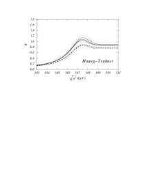
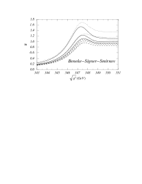
Figure 2: The total normalised photon-induced $t\bar{t}$ cross section $R$ at the LC versus the c.m. energy in the threshold regime at LO (dotted curves), NLO (dashed) and NNLO (solid). Hoang–Teubner used the 1S mass scheme with $m_{t}^{1S}=173.68$ GeV, Melnikov–Yelkhovsky the kinetic mass at $15$ GeV with $m_{t,15\,\mbox{\scriptsize GeV}}^{\rm kin}=173.10$ GeV, and Beneke–Signer–Smirnov and Yakovlev the PS mass at $20$ GeV with $m_{t,20\,\mbox{\scriptsize GeV}}^{\rm PS}=173.30$ GeV. The plots have been generated from results provided by the groups Hoang–Teubner (HT), Melnikov–Yelkhovsky (MY) and Beneke–Signer–Smirnov (BSS) and Yakovlev.

Order	LO			NLO			NNLO
$\mu_{\rm soft}$[GeV]	$15$	$30$	$60$	$15$	$30$	$60$	$15$	$30$	$60$
HT ($m_{t}^{1S}$)	$1.22$	$0.96$	$0.80$	$0.86$	$0.90$	$0.88$	$1.14$	$1.08$	$1.04$
	$347.51$	$347.65$	$347.88$	$347.53$	$347.56$	$347.57$	$347.53$	$347.48$	$347.46$
MY ($m^{\rm kin}_{t,15~{}\mbox{\scriptsize GeV}}$)	$1.70$	$1.28$	$1.03$	$0.80$	$0.86$	$0.87$	$1.33$	$1.15$	$1.06$
	$347.05$	$347.33$	$347.63$	$347.69$	$347.59$	$347.58$	$347.50$	$347.54$	$347.54$
BSS ($m^{\rm PS}_{t,20~{}\mbox{\scriptsize GeV}}$)	$1.69$	$1.27$	$1.03$	$1.09$	$1.03$	$0.96$	$1.53$	$1.23$	$1.11$
	$347.47$	$347.74$	$348.05$	$347.69$	$347.71$	$347.73$	$347.33$	$347.51$	$347.59$

Table 4: The values of $R$ (upper numbers) at the respective peak position (lower numbers in units of GeV) at LO, NLO and NNLO. Hoang-Teubner used the 1S mass scheme with $m_{t}^{1S}=173.68$ GeV, Melnikov–Yelkhovsky the kinetic mass at $15$ GeV with $m_{t,15\,\mbox{\scriptsize GeV}}^{\rm kin}=173.10$ GeV, and Beneke-Signer-Smirnov the PS mass at $20$ GeV with $m_{t,20\,\mbox{\scriptsize GeV}}^{\rm PS}=173.30$ GeV. The values have been determined from results provided by the groups Hoang–Teubner (HT), Melnikov–Yelkhovsky (MY) and Beneke–Signer–Smirnov (BSS).

The three threshold masses eliminate the large higher order corrections to the peak position mentioned above. In addition, they can reduce the correlation of the peak position to the value of the strong coupling and theoretical parameters, such as the renormalisation scale $\mu_{\rm soft}$. For the 1S mass this is achieved automatically; for the PS and the kinetic mass this is achieved by setting $\mu_{f}$ to a value of order $M_{t}\alpha_{s}\approx 15$–$20$ GeV. (Choosing $\mu_{f}$ much smaller than $M_{t}\alpha_{s}$ also eliminates the large corrections at high orders, but does not reduce the correlation to $\mu_{\rm soft}$ and $\alpha_{s}$ in a significant way [18].) In Tables 2 and 3 numerical values of the top quark PS mass for $\mu_{f}^{\rm PS}=20$ GeV, the 1S mass, and the kinetic mass for $\mu_{f}^{\rm kin}=15$ GeV are given, taking the $\overline{\mbox{MS}}$ mass $\overline{m}_{t}(\overline{m}_{t})=160,165,170$ GeV as a reference point and using $\alpha_{s}(165~{}\mbox{GeV})=0.1066,0.1091,0.1117$. As a comparison, also the corresponding values for the top quark pole mass have been displayed in Table 3. The knowledge of the two- [47] and three-loop corrections [48, 49] in the relation between the pole and the $\overline{\mbox{MS}}$ mass are required to obtain the two- and three-loop values of the PS, 1S and kinetic mass. For the PS, 1S and pole masses the relation to the $\overline{\mbox{MS}}$ mass is known at three loops and for the kinetic mass at two loops. For the PS mass the four-loop contributions in the “large-$\beta_{0}$” limit have been derived from the expression for the Borel transform of the static potential [43] and of the difference between the pole and the $\overline{\mbox{MS}}$ mass [50]. The same information is in principle sufficient to determine the four-loop “large-$\beta_{0}$” correction in the difference between the 1S and the $\overline{\mbox{MS}}$ mass. For the kinetic mass the three-loop contributions in the “large-$\beta_{0}$” limit have been determined in [46]. (The three-loop “large-$\beta_{0}$” corrections in the relation between the kinetic and the $\overline{\mbox{MS}}$ mass have been obtained using Eq. (21) in the preprint version of Ref. [46].) In Tables 2 and 3 the large-$\beta_{0}$ corrections are indicated by a star. We emphasise that the numbers shown in these tables do not contain any electroweak corrections. The latter can amount to shifts at the $1$ GeV level [51].

The numbers displayed in the tables show an excellent convergence of the perturbative relation between the threshold masses and the $\overline{\mbox{MS}}$ mass. For $\alpha_{s}(M_{Z})=0.119$ and $\overline{m}_{t}(\overline{m}_{t})=165$ GeV the one-, two-, three- and the available four-loop large-$\beta_{0}$ corrections for the threshold masses are $6.7$–$7.2$, $1.2$, $0.2$–$0.3$ and $0.1$ GeV, respectively. The corresponding corrections in the relation between the pole mass and $\overline{m}_{t}(\overline{m}_{t})$ read $7.6$, $1.6$, $0.5$ and $0.3$ GeV. For the pole mass the three-loop corrections are about a factor two and the four-loop large-$\beta_{0}$ corrections a factor three larger. This behaviour is caused by the infrared-sensitivity of the pole mass and corresponds to the ambiguity of the pole mass of order $\Lambda_{\rm QCD}$. The numbers displayed in the tables also show that a shift in $\alpha_{s}(M_{Z})$ by $0.001$ corresponds to a shift of about $70$ MeV in the threshold masses.

In the framework of the Linear Collider Workshop several presentations were given by M. Beneke, A. H. Hoang, K. Melnikov, Y. Sumino, T. Teubner and O. Yakovlev of, in part, preliminary results for the cross section using threshold masses. The following discussion provides a summary of these results, choosing one representative example for each of the three threshold mass definitions. The results for the discussion have been provided by HT in the 1S scheme for $m_{t}^{1S}=173.68$ GeV, by Melnikov–Yelkhovsky (MY) in the kinetic mass scheme for $m^{\rm kin}_{t,15\,\mbox{\scriptsize GeV}}=173.10$ GeV, and by BSS in the PS mass scheme for $m^{\rm PS}_{t,20\,\mbox{\scriptsize GeV}}=173.30$ GeV. The numerical values of the respective threshold masses are the known highest order entries in Tables 2 and 3 for common $\alpha_{s}(M_{Z})=0.119$ and $\overline{m}_{t}(\overline{m}_{t})=165$ GeV. HT and BSS used the codes developed for Refs. [14] and [17], respectively. Yakovlev and NOS have also provided results in the PS mass scheme. Their results are in qualitative agreement with those of BSS. In Figs. 2 the total normalised photon-induced cross section $R$ is displayed at LO (dotted lines), NLO (dashed lines) and NNLO (solid lines) using the three threshold masses mentioned above for $\alpha_{s}(M_{Z})=0.119$ and $\mu_{\rm soft}=15$, $30$, $60$ GeV, and ignoring the effects of beamstrahlung and initial state radiation. The values of $R$ (upper number) at the respective peak position (lower number in units of GeV) are given in Table 4.

The threshold masses have been implemented employing the non-relativistic power-counting rules for the perturbative series describing the difference between threshold and pole mass. This means that for all threshold masses the one-loop corrections displayed in Eqs. (10–12) have been treated as LO in the non-relativistic expansion, the two-loop corrections as NLO and so on. The results in Figs. 2 and Table 4 show that the peak positions obtained with different threshold masses converge when higher orders are included. This is a consequence of the fact that the numerical values of all the threshold masses have been determined from $\overline{m}_{t}(\overline{m}_{t})=165$ GeV as a reference value. Compared to the results in the pole mass scheme displayed in Sec. 3, the results in Figs. 2 and Table 4 show an improved stability of the peak position with respect to the size of higher order corrections, and with respect to the sensitivity to changes in $\mu_{\rm soft}$. For $\mu_{\rm soft}=15/30/60$ GeV, the NLO (NNLO) shifts of the peak position are $20/-90/-310$ MeV ($0/-80/-110$ MeV) for HT in the 1S scheme, $640/260/-50$ MeV ($-190/-50/-40$ MeV) for MY in the kinetic mass scheme and $220/-30/-330$ MeV ($-360/-200/-140$ MeV) for BSS in the PS scheme. The lack of convergence that can be observed for some numbers is not an indication of large unknown higher order corrections, but a consequence of the fact that the threshold masses that have been used for the analysis partially lead to NLO shifts that are much smaller than the parametric accuracy that can be achieved at the NLO level. A better quantification is obtained by comparing the shift from LO directly to NNLO with the corresponding shift, when the cross section is plotted for fixed pole mass as in Figs. 1. The variation of the peak position when $\mu_{\rm soft}$ is varied between $15$ and $60$ GeV at LO/NLO/NNLO is $370/40/70$ MeV for HT in the 1S scheme, $580/110/40$ MeV for MY in the kinetic mass scheme and $580/40/260$ MeV for BSS in the PS scheme. The scale variation of the peak position at NNLO obtained by BSS in the PS mass scheme is by a factor of 4–5 larger than the corresponding variation obtained by HT in the 1S and by MY in the kinetic mass scheme. The fact that the stability of the results in the PS mass scheme is worse than in the 1S and the kinetic mass scheme might originate from the fact that the difference between the PS and the pole mass contains only corrections from the static potential. The 1S and the kinetic mass contain additional corrections, which are subleading in the non-relativistic velocity counting. However, it should be noted that the stability of the peak position for a fixed threshold mass is not necessarily a useful quantification of the theoretical error. A mass definition that would be equal to the peak position, for example, would lead to no variation at all. The shifts of the peak position quoted above should therefore be considered in conjunction with the variation of the threshold mass values with the order of perturbation theory given in Tables 2 and 3.

From the size of the NNLO corrections to the peak positions and from the scale variation of the peak positions at NNLO, we estimate that the current theoretical uncertainty of a determination of the threshold masses from the peak position based on the NNLO calculations is about $100$ MeV. (The uncertainty coming from the different calculational methods used by the various groups has been estimated in Sec. 3 and is included in this number.) In Refs. [52, 40, 41] the ultrasoft corrections and the leading logarithmic contributions proportional to $\ln\alpha_{s}$ were calculated for the mass of a fictitious toponium 1S state at NNNLO. Up to corrections coming from the top width (and other electroweak corrections), the toponium 1S mass is equal to the location of the peak of $R$. As for the normalisation, these corrections can be used as a consistency check for the error estimate of the top mass extraction based on the NNLO corrections alone. Both types of corrections amount to about $200$ MeV, corresponding to a shift of $100$ MeV in the top quark mass. This supports the error estimate based on the NNLO calculations alone. However, as for the case of the normalisation, a concrete statement about the true size of the NNNLO corrections can only be drawn once the full NNNLO corrections have been determined. Taking into account four-loop corrections in the relation between the threshold masses and the $\overline{\mbox{MS}}$ mass, $\overline{m}_{t}(\overline{m}_{t})$ can be determined with comparable precision for an uncertainty in $\alpha_{s}(M_{Z})$ of around $0.001$–$0.002$. Realistic simulation studies [9] have shown that these conclusions remain valid if beam effects from initial state radiation or beamstrahlung are taken into account.

The threshold masses do not lead to an improvement of the stability in the normalisation of $R$ because their main effect is to redefine the binding energy of the $t\bar{t}$ system. An energy shift leaves the wave function of the $t\bar{t}$ system unaffected and, therefore, cannot affect higher order corrections to the normalisation.

5 Summary and Open Issues

In this article the results for the NNLO QCD calculations for the total photon-mediated $t\bar{t}$ production cross section obtained by different groups have been compared. A detailed assessment of the dependence of the individual results on the calculational techniques, the intermediate regularization prescriptions and the treatment of higher order corrections has been carried out. As far as the determination of the top quark mass from the position of the peak in the total cross section is concerned, the uncertainty caused by the use of different methods is around 50–80 MeV. Using the top quark pole mass to parameterise the total cross section, the latter uncertainty is negligible with respect to the perturbative uncertainty in an extraction of the pole mass parameter, which is estimated to be around 300 MeV. This estimate matches formal arguments based on the analysis of the large order behaviour of perturbation theory, which state that the pole mass cannot be determined to a precision better than ${\cal{O}}(\Lambda_{\rm QCD})$. Using so-called “threshold masses”, which lead to a much better high order behaviour and which preserve the non-relativistic velocity counting, the uncertainty in the mass extraction is around 100 MeV. The top quark $\overline{\mbox{MS}}$ mass $\overline{m}_{t}(\overline{m}_{t})$ can be determined with comparable precision if $\alpha_{s}(M_{Z})$ is known with an uncertainty of $0.001$–$0.002$. (An uncertainty in $\alpha_{s}(M_{Z})$ of $0.001$ corresponds to an uncertainty of 70 MeV in $\overline{m}_{t}(\overline{m}_{t})$.) Realistic simulation studies have shown that these conclusions remain valid if realistic beam effects are taken into account. For the normalisation of the total cross section, we find that the NNLO corrections are much larger than indicated by the renormalisation scale dependence of the NLO results. The normalisation at NNLO also has a considerable dependence on calculational methods and the renormalisation scale $\mu_{\rm soft}$. We estimate the uncertainty of the normalisation of the NNLO cross section as around 20%, which seems to jeopardise accurate measurements of top quark couplings or the total top quark width. The calculation of NNNLO corrections will be mandatory to reduce the current uncertainties in the normalisation of the total cross section. At present, the most difficult parts of a complete NNNLO QCD calculation of the total cross section seem to be the three-loop corrections to the static potential and the short-distance coefficient $C$. Another way to get information about the size of higher order corrections is to resum logarithmic contributions to all orders in perturbation theory using the renormalisation group evolution of the operators in the non-relativistic effective theory for $t\bar{t}$ close to threshold. First attempts at carrying out such a resummation consistently have been made in Refs. [17, 53].

Except for the NNLO calculations of the top three momentum distribution in Refs. [18, 14], practically nothing is known about the size of NNLO corrections to differential observables. In view of the large NNLO QCD corrections to the total cross section, calculations of the complete NNLO corrections to differential observables, such as the top momentum distribution, the forward–backward asymmetry and certain leptonic spectra, are needed to obtain realistic estimates of the theoretical uncertainties. A first step toward this aim is the development of a consistent and systematic approach to account for electroweak effects. The present calculations of the total $t\bar{t}$ cross section at NNLO have only taken into account relativistic corrections in the framework of QCD. So far, electroweak effects have been taken into account, mainly by shifting the energy in the Schrödinger equation (1) into the upper complex plane by $i\Gamma_{t}$. This treatment accounts for all electroweak effects at LO in the non-relativistic expansion. At NLO electroweak effects lead to final state interactions originating from the exchange of gluons between the top quarks and their decay products. These corrections are called “non-factorisable” (or “rescattering”) corrections because they can in general not be unambiguously considered as being either corrections to $t\bar{t}$ production or to top quark decay. For the total cross section it has been shown that the non-factorisable corrections cancel at NLO and that the net effect of the electroweak corrections reduces to shifting the c.m. energy by $i\,\Gamma_{t}$ [54]. For a number of differential observables, such as the top quark momentum distribution and the energy spectrum of leptons originating from the decay of a W-boson, NLO non-factorisable corrections have been calculated [8] and shown to be of order 10%, as can be expected for ${\cal{O}}(\alpha_{s})$ corrections. No consistent and systematic prescription to implement electroweak effects at NNLO has been developed yet, and practically nothing is known about the size of the non-factorisable corrections beyond NLO.

References

- [1] J. H. Kühn, Act. Phys. Pol. B 12 (1981) 347.
- [2] I. I. Bigi, Y. L. Dokshitzer, V. A. Khoze, J. H. Kühn and P. Zerwas, Phys. Lett. B 181 (1986) 157.
- [3] V. S. Fadin and V. A. Khoze, Zh. Eksp. Teor. Fiz. 46 (1987) 417 [JETP Lett. 46 (1987) 525].
- [4] M. J. Strassler and M. E. Peskin, Phys. Rev. D 43 (1991) 1500.
- [5] M. Jeżabek, J. H. Kühn and T. Teubner, Z. Phys. C 56 (1992) 653.
- [6] Y. Sumino, K. Fujii, K. Hagiwara, H. Murayama and C.-K. Ng, Phys. Rev. D 47 (1993) 56.
- [7] H. Murayama and Y. Sumino, Phys. Rev. D 47 (1993) 82; R. Harlander, M. Jeżabek, J. H. Kühn and T. Teubner, Phys. Lett. B 346 (1995) 137.
- [8] R. Harlander, M. Jeżabek, J. H. Kühn and M. Peter, Z. Phys. C 73 (1997) 477; M. Peter and Y. Sumino, Phys. Rev. D 57 (1998) 6912.
- [9] D. Peralta, M. Martinez and R. Miquel, talk presented at the 4th International Workshop on Linear Colliders, Sitges, Barcelona, Spain, April 28 - May 5 1999.
- [10] K. Fujii, T. Matsui and Y. Sumino, Phys. Rev. D 50 (1994) 4341.
- [11] P. Comas, R. Miquel, M. Martinez and S. Orteu, talk given at Physics with Linear Colliders, 1995, published in Linear Collisions at GeV, DESY 96-123D (1996) 57.
- [12] D. Cinabro, talk presented at the 4th International Workshop on Linear Colliders, Sitges, Barcelona, Spain, April 28 - May 5 1999.
- [13] A. H. Hoang and T. Teubner, Phys. Rev. D 58 (1998) 114023.
- [14] A. H. Hoang and T. Teubner, Phys. Rev. D 60 (1999) 114027.
- [15] K. Melnikov and A. Yelkhovsky, Nucl. Phys. B 528 (1998) 59.
- [16] O. Yakovlev, Phys. Lett. B 457 (1999) 170.
- [17] M. Beneke, A. Signer and V. A. Smirnov, Phys. Lett. B 454 (1999) 137.
- [18] T. Nagano, A. Ota and Y. Sumino, Phys. Rev. D 60 (1999) 114014.
- [19] A. A. Penin and A. A. Pivovarov, Nucl. Phys. B 550 (1999) 375; University of Mainz preprint, MZ-TH-98-61 [hep-ph/9904278].
- [20] V. S. Fadin and V. A. Khoze, Yad. Fiz. 48 (1988) 487 [Sov. J. Nucl. Phys. 48 (1988) 309].
- [21] W. Kwong, Phys. Rev. D 43 (1991) 1488.
- [22] M. Beneke, Phys. Lett. B 434 (1998) 115.
- [23] A. H. Hoang, M. C. Smith, T. Stelzer and S. S. Willenbrock, Phys. Rev. D 59 (1999) 114014.
- [24] N. Uraltsev, talk given at the International School of Physics “Enrico Fermi”: Heavy Flavor Physics - A Probe of Nature’s Grand Design, Varenna, Italy, July 8–18, 1997 [hep-ph/9804275].
- [25] V. S. Fadin and V. A. Khoze, Yad. Fiz. 53 (1991) 1118 [Sov. J. Nucl. Phys. 53 (1991) 692].
- [26] J. H. Kühn and T. Teubner, Eur. Phys. J. C 9 (1999) 221.
- [27] W. Fischler, Nucl. Phys. B 129 (1977) 157; A. Billoire, Phys. Lett. B 92 (1980) 343.
- [28] R. Karplus and A. Klein, Phys. Rev. 87 (1952) 848.
- [29] Y. Schröder, Phys. Lett. B 447 (1999) 321; M. Peter, Phys. Rev. Lett. 78 (1997) 602; Nucl. Phys. B 501 (1997) 471.
- [30] M. Beneke and V. A. Smirnov, Nucl. Phys. B 522 (1998) 321.
- [31] A. Czarnecki and K. Melnikov, Phys. Rev. Lett. 80 (1998) 2531; M. Beneke, A. Signer and V. A. Smirnov, Phys. Rev. Lett. 80 (1998) 2535.
- [32] P. Labelle, Phys. Rev. D 58 (1998) 093013 [hep-ph/9608491]; A. V. Manohar, Phys. Rev. D 56 (1997) 230; M. Luke and A. V. Manohar, Phys. Rev. D 55 (1997) 4129; B. Grinstein and I. Z. Rothstein, Phys. Rev. D 57 (1998) 78; M. Luke and M. J. Savage, Phys. Rev. D 57 (1998) 413; H. W. Grießhammer, Phys. Rev. D 58 (1998) 094027; University of Washington preprint, NT-UW-98-22 [hep-ph/9810235].
- [33] A. Pineda and J. Soto, Nucl. Phys. Proc. Suppl. 64 (1998) 428; Phys. Rev. D 59 (1999) 016005; N. Brambilla, A. Pineda, J. Soto and A. Vairo, [hep-ph/9907240].
- [34] W. E. Caswell and G. E. Lepage, Phys. Lett. B 167 (1986) 437.
- [35] G. T. Bodwin, E. Braaten and G. P. Lepage, Phys. Rev. D 51 (1995) 1125; Phys. Rev. D 55 (1997) 5853 (Erratum).
- [36] A. H. Hoang, Phys. Rev. D 56 (1998) 5851.
- [37] M. Beneke and V. M. Braun, Nucl. Phys. B 426 (1994) 301; I. I. Bigi et al., Phys. Rev. D 50 (1994) 2234.
- [38] M. C. Smith and S. S. Willenbrock, Phys. Rev. Lett. 79 (1997) 3825.
- [39] I. I. Bigi, M. Shifman, N. Uraltsev and A. Vainshtein, Phys. Rev. D 56 (1997) 4017.
- [40] B. A. Kniehl and A. Penin, University of Hamburg preprint, DESY-99-099 [hep-ph/9907489].
- [41] B. A. Kniehl and A. Penin, University of Hamburg preprint, DESY-99-173 [hep-ph/9911414].
- [42] V. S. Fadin, O. I. Yakovlev, Yad. Fiz. 53 (1991) 688 [Sov. J. Nucl. Phys. 53 (1991) 111].
- [43] U. Aglietti and Z. Ligeti, Phys. Lett. B 364 (1995) 75.
- [44] M. Jeżabek, talk given at Zeuthen Workshop on Elementary Particle Theory: Physics at LEP200 and Beyond, Teupitz, Germany, April 10–15, 1994, published in Nucl. Phys. Proc. Suppl. 37 (1994) 197; M. Jeżabek, J. H. Kühn and T. Teubner, talk given at Physics with Linear Colliders, 1993; published in Linear Collisions at GeV, DESY 93-123C (1993) 303.
- [45] A. Pineda and F. J. Yndurain, Phys. Rev. D 58 (1998) 094022.
- [46] A. Czarnecki, K. Melnikov and N. Uraltsev, Phys. Rev. Lett. 80 (1998) 3189.
- [47] N. Gray, D. J. Broadhurst, W. Grafe and K. Schilcher, Z. Phys. C 48 (1990) 673.
- [48] K. G. Chetyrkin and M. Steinhauser, Phys. Rev. Lett. 83 (1999) 4001; University Hamburg preprint, DESY-99-174 [hep-ph/9911434].
- [49] K. Melnikov and T. v. Ritbergen, SLAC preprint, SLAC-PUB-8321 [hep-ph/9912391].
- [50] M. Beneke and V. M. Braun, Phys. Lett. B 348 (1995) 513.
- [51] R. Hempfling and B. A. Kniehl, Phys. Rev. D 51 (1995) 1386.
- [52] N. Brambilla, A. Pineda, J. Soto and A. Vairo, CERN preprint, CERN-TH-99-301 [hep-ph/9910238].
- [53] M. E. Luke, A. V. Manohar and I. Z. Rothstein, University of San Diego preprint, UCSD-PTH-99-11 [hep-ph/9910209]; A. V. Manohar and I. W. Stewart, University of San Diego preprint, UCSD-PTH-99-23 [hep-ph/9912226].
- [54] V. S. Fadin, V. A. Khoze and A. D. Martin, Phys. Lett. B 320 (1994) 141; Phys. Rev. D 49 (1994) 2247; K. Melnikov and O. Yakovlev, Phys. Lett. B 324 (1994) 217.