SUPERSYMMETRY IN PARTICLE PHYSICS:
THE RENORMALIZATION GROUP VIEWPOINT^†

D. I. Kazakov

BLTP, JINR, Dubna and ITEP, Moscow
e-mail: kazakovd@thsun1.jinr.ru

Abstract

An attempt is made to present modern hopes to find manifestation of supersymmetry, a new symmetry that relates bosons and fermions, in particle physics from the point of view of renormalization group flow. The Standard Model of particle interactions is briefly reviewed, the main notions of supersymmetry are introduced. In more detail the RG flow in the Minimal Supersymmetric Standard Model is considered. Predictions of particle spectrum are obtained based on the RG fixed points.

———————————————

^† Review talk given at the Conference “Renormalization Group at the Turn of the Millennium”, Taxco, Mexico, January 1999

References 41

1 Introduction

1.1 The Standard Model

The Standard Model (SM) of fundamental interactions describes strong, weak and electromagnetic interactions of elementary particles [1]. It is based on a gauge principle, according to which all the forces of Nature are mediated by an exchange of the gauge fields of a corresponding local symmetry group. The symmetry group of the SM is

$$SU_{colour}(3)\otimes SU_{left}(2)\otimes U_{hypercharge}(1),$$ (1.1)

whereas the field content is the following:

Gauge sector :  Spin = 1

The gauge bosons are spin 1 vector particles belonging to the adjoint representation of the group (1.1). Their quantum numbers with respect to $SU(3)\otimes SU(2)\otimes U(1)$ are:

$$\begin{array}[]{ccccc}\mbox{\em gluons}&G_{\mu}^{a}:&\ (\underline{8},\underline{1},0)&\ \ SU_{c}(3)&\ \ g_{s},\\ {\begin{array}[]{cc}\mbox{\em intermediate}\\ \mbox{\em weak bosons}\end{array}}&W_{\mu}^{i}:&\ (\underline{1},\underline{3},0)&\ \ SU_{L}(2)&\ \ g,\\ \mbox{\em abelian boson}&B_{\mu}:&\ (\underline{1},\underline{1},0)&\ \ U_{Y}(1)&\ \ g^{\prime},\end{array}$$

where the coupling constants are usually denoted by $g_{s}$, $g$ and $g^{\prime}$, respectively.

Fermion sector :   Spin = 1/2

The matter fields are fermions belonging to the fundamental representation of the gauge group. These are believed to be quarks and leptons of at least of three generations. The SM is left-right asymmetric. Left-handed and right-handed fermions have different quantum numbers:

$$\begin{array}[]{cccccccc}\mbox{\em quarks}&&&&&&&\\ Q_{\alpha L}^{i}=&\left(\begin{array}[]{c}U_{\alpha}^{i}\\ D_{\alpha}^{i}\end{array}\right)_{L}&=&\left(\begin{array}[]{c}u^{i}\\ d^{i}\end{array}\right)_{L},&\left(\begin{array}[]{c}c^{i}\\ s^{i}\end{array}\right)_{L},&\left(\begin{array}[]{c}t^{i}\\ b^{i}\end{array}\right)_{L},&\ldots&(\underline{3},\underline{2},1/3)\\ &U_{\alpha R}^{i}&=&u_{iR},&c_{iR},&t_{iR},&\ldots&(\underline{3}^{*},\underline{1},4/3)\\ &D_{\alpha R}^{i}&=&d_{iR},&s_{iR},&b_{iR},&\ldots&(\underline{3}^{*},\underline{1},-2/3)\\ \mbox{\em leptons}&L_{\alpha L}&=&\left(\begin{array}[]{c}\nu_{e}\\ e\end{array}\right)_{L},&\left(\begin{array}[]{c}\nu_{\mu}\\ \mu\end{array}\right)_{L},&\left(\begin{array}[]{c}\nu_{\tau}\\ \tau\end{array}\right)_{L},&\ldots&(\underline{1},\underline{2},-1)\\ &E_{\alpha R}&=&e_{R},&\mu_{R},&\tau_{R},&\ldots&(\underline{1},\underline{1},-2)\end{array}$$

$i=1,2,3$ - colour, $\alpha=1,2,3,\ldots$ - generation.

Higgs sector :   Spin = 0

In the minimal version of the SM there is one doublet of Higgs scalar fields

$$H=\left(\begin{array}[]{c}H^{0}\\ H^{-}\end{array}\right)\ \ \ \ (\underline{1},\underline{2},-1),$$ (1.2)

which is introduced in order to give masses to quarks, leptons and intermediate weak bosons via spontaneous breaking of electroweak symmetry.

In Quantum Field Theory framework the SM is described by the following Lagrangian

$${\cal L}={\cal L}_{gauge}+{\cal L}_{Yukawa}+{\cal L}_{Higgs},$$ (1.3)

$${\cal L}_{gauge} = -\frac{1}{4}G_{\mu\nu}^{a}G_{\mu\nu}^{a}-\frac{1}{4}W_{\mu\nu}^{i}W_{\mu\nu}^{i}-\frac{1}{4}B_{\mu\nu}B_{\mu\nu}$$

$$+i\overline{L}_{\alpha}\gamma^{\mu}D_{\mu}L_{\alpha}+i\overline{Q}_{\alpha}\gamma^{\mu}D_{\mu}Q_{\alpha}+i\overline{E}_{\alpha}\gamma^{\mu}D_{\mu}E_{\alpha}$$

$$+i\overline{U}_{\alpha}\gamma^{\mu}D_{\mu}U_{\alpha}+i\overline{D}_{\alpha}\gamma^{\mu}D_{\mu}D_{\alpha}+(D_{\mu}H)^{\dagger}(D_{\mu}H),$$

where

$$G_{\mu\nu}^{a} = \partial_{\mu}G_{\nu}^{a}-\partial_{\nu}G_{\mu}^{a}+g_{s}f^{abc}G_{\mu}^{b}G_{\nu}^{c},$$

$$W_{\mu\nu}^{i} = \partial_{\mu}W_{\nu}^{i}-\partial_{\nu}W_{\mu}^{i}+g\epsilon^{ijk}W_{\mu}^{j}W_{\nu}^{k},$$

$$B_{\mu\nu} = \partial_{\mu}B_{\nu}-\partial_{\nu}B_{\mu},$$

$$D_{\mu}L_{\alpha} = (\partial_{\mu}-i\frac{g}{2}\tau^{i}W_{\mu}^{i}+i\frac{g^{\prime}}{2}B_{\mu})L_{\alpha},$$

$$D_{\mu}E_{\alpha} = (\partial_{\mu}+ig^{\prime}B_{\mu})E_{\alpha},$$

$$D_{\mu}Q_{\alpha} = (\partial_{\mu}-i\frac{g}{2}\tau^{i}W_{\mu}^{i}-i\frac{g^{\prime}}{6}B_{\mu}-i\frac{g_{s}}{2}\lambda^{a}G_{\mu}^{a})Q_{\alpha},$$

$$D_{\mu}U_{\alpha} = (\partial_{\mu}-i\frac{2}{3}g^{\prime}B_{\mu}-i\frac{g_{s}}{2}\lambda^{a}G_{\mu}^{a})U_{\alpha},$$

$$D_{\mu}D_{\alpha} = (\partial_{\mu}+i\frac{1}{3}g^{\prime}B_{\mu}-i\frac{g_{s}}{2}\lambda^{a}G_{\mu}^{a})D_{\alpha}.$$

$${\cal L}_{Yukawa}=y_{\alpha\beta}^{L}\overline{L}_{\alpha}E_{\beta}H+y_{\alpha\beta}^{D}\overline{Q}_{\alpha}D_{\beta}H+y_{\alpha\beta}^{U}\overline{Q}_{\alpha}U_{\beta}\tilde{H}+h.c.,$$ (1.5)

where $\tilde{H}=i\tau_{2}H^{\dagger}$.

$${\cal L}_{Higgs}=-V=m^{2}H^{\dagger}H-\frac{\lambda}{2}(H^{\dagger}H)^{2}.$$ (1.6)

Here $\{y\}$ are the Yukawa and $\lambda$ is the Higgs coupling constants, both dimensionless, and $m$ is the only dimensional mass parameter.

The Lagrangian of the SM contains the following set of free parameters:

• 3 gauge couplings $g_{s},g,g^{\prime}$;

• 3 Yukawa matrices $y_{\alpha\beta}^{L},y_{\alpha\beta}^{D},y_{\alpha\beta}^{U}$;

• Higgs coupling constant $\lambda$;

• Higgs mass parameter $m^{2}$;

• number of matter fields (generations).

All the particles obtain their masses due to spontaneous breaking of $SU_{left}(2)$ symmetry group via a non-zero vacuum expectation value (v.e.v.) of the Higgs field

$$<H>=\left(\begin{array}[]{c}v\\ 0\end{array}\right),\ \ \ \ v=m/\sqrt{\lambda}.$$ (1.7)

As a result the gauge group of the SM is spontaneously broken down to

$$SU_{c}(3)\otimes SU_{L}(2)\otimes U_{Y}(1)\Rightarrow SU_{c}(3)\otimes U_{EM}(1).$$

The physical weak intermediate bosons are the linear combinations of the gauge ones

$$W_{\mu}^{\pm}=\frac{W_{\mu}^{1}\mp iW_{\mu}^{2}}{\sqrt{2}},\ \ \ \ Z_{\mu}=-\sin{\theta_{W}}B_{\mu}+\cos{\theta_{W}}W_{\mu}^{3}$$ (1.8)

with masses

$$m_{W}=\frac{1}{\sqrt{2}}gv,\ \ \ \ m_{Z}=m_{W}/\cos{\theta_{W}},\ \ \ \ \tan{\theta_{W}}=g^{\prime}/g,$$ (1.9)

while the photon field

$$\gamma_{\mu}=\cos{\theta_{W}}B_{\mu}+\sin{\theta_{W}}W_{\mu}^{3}$$ (1.10)

remains massless.

The matter fields acquire masses proportional to the corresponding Yukawa couplings:

$$M_{\alpha\beta}^{u}=y_{\alpha\beta}^{u}v,\ M_{\alpha\beta}^{d}=y_{\alpha\beta}^{d}v,\ M_{\alpha\beta}^{l}=y_{\alpha\beta}^{l}v,\ m_{H}=\sqrt{2}m.$$ (1.11)

Explicit mass terms in the Lagrangian are forbidden because they are not $SU_{left}(2)$ symmetrical and would destroy the renormalizability of the Standard Model.

The SM has been constructed as a result of numerous efforts both theoretical and experimental. At present the SM is extraordinary successful, the achieved accuracy of its predictions corresponds to the experimental data within 5 % [2]. All the particles except for the Higgs boson have been discovered experimentally.

However the SM has its natural drawbacks and unsolved problems. Among them are:

• large number of free parameters,

• formal unification of strong and electroweak interactions,

• the Higgs boson has not yet been observed and it is not clear whether it is fundamental or composite,

• the problem of CP-violation is not well understood including CP-violation in strong interaction,

• flavour mixing and the number of generations are arbitrary,

• the origin of the mass spectrum is unclear.

The answer to these problems lies beyond the SM.

1.2 RG flow in the Standard Model

The question is: how to go beyond the SM? Apparently we are talking about new particles, new structures, new interactions and new symmetries. The answer is not obvious. We describe below one of the options and assume that at high energies (small distances) fundamental interactions possess wider symmetries, in particular, new kind of symmetry, symmetry between bosons and fermions, called sypersymmetry. This is a wide subject by itself, however, we would like to look at it from the point of view of renormalization group. Let us try to go along the road offered by the renormalization group flow.

Let us take the Lagrangian of the SM and see what happens with its parameters (the couplings) when the energy scale increases. As it follows from eq.(1.1) one has three gauge couplings corresponding to $SU(3)_{c}\times SU(2)_{L}\times U(1)_{Y}$ gauge groups, $g_{s},g$ and $g^{\prime}$, respectively. In what follows it will be more useful to consider the set $\{g_{1},g_{2},g_{3}\}=\{\sqrt{3/5}g^{\prime},g,g_{s}\}$. Besides, there are three Yukawa couplings $y_{U},y_{D}$ and $y_{L}$, which are $3\times 3$ matrices in the generation space and one Higgs coupling $\lambda$.

To simplify the picture we consider only the third generation Yukawa couplings replacing the Yukawa matrices by their $(3,3)$ elements. Then the RG equations in the leading one-loop order are [3] :

$$\frac{d{\mbox{a}}_{i}}{dt} = b_{i}{\mbox{a}}_{i}^{2},\ \ \ \ \ t=\log(Q^{2}/\mu^{2}),$$ (1.12)

$$\frac{dY_{t}}{dt} = -Y_{t}\left(8{\mbox{a}}_{3}+\frac{9}{4}{\mbox{a}}_{2}+\frac{17}{20}{\mbox{a}}_{1}-\frac{9}{2}Y_{t}\right),$$

$$\frac{dY_{b}}{dt} = -Y_{b}\left(8{\mbox{a}}_{3}+\frac{9}{4}{\mbox{a}}_{2}+\frac{1}{4}{\mbox{a}}_{1}-\frac{3}{2}Y_{t}\right),$$ (1.13)

$$\frac{dY_{\tau}}{dt} = -Y_{\tau}\left(\frac{9}{4}{\mbox{a}}_{2}+\frac{9}{4}{\mbox{a}}_{1}-3Y_{t}\right),$$

$$\frac{d\lambda}{dt} = \frac{9}{8}{\mbox{a}}_{2}^{2}+\frac{9}{20}{\mbox{a}}_{2}{\mbox{a}}_{1}+\frac{27}{200}{\mbox{a}}_{1}^{2}-\frac{9}{2}{\mbox{a}}_{2}\lambda-\frac{9}{10}{\mbox{a}}_{1}\lambda+6\lambda Y_{t}-6Y_{t}^{2}+6\lambda^{2},$$ (1.14)

where to simplify the formulas we have used the notation

$${\mbox{a}}_{i}\equiv\frac{\alpha_{i}}{4\pi}\equiv\frac{g_{i}^{2}}{16\pi^{2}},\ \ \ (i=1,2,3),\ \ \ Y_{k}\equiv\frac{(y^{k}_{33})^{2}}{16\pi^{2}},\ \ \ (k=t,b,\tau).$$

For the SM the coefficients $b_{i}$ are:

$$b_{i}=\left(\begin{array}[]{r}b_{1}\\ b_{2}\\ b_{3}\end{array}\right)=\left(\begin{array}[]{r}0\\ -22/3\\ -11\end{array}\right)+N_{Fam}\left(\begin{array}[]{r}4/3\\ 4/3\\ 4/3\end{array}\right)+N_{Higgs}\left(\begin{array}[]{r}1/10\\ 1/6\\ 0\end{array}\right).$$ (1.15)

Here $N_{Fam}$ is the number of generations of matter multiplets and $N_{Higgs}$ is the number of Higgs doublets. We use $N_{Fam}=3$ and $N_{Higgs}=1$ for the minimal SM.

The initial conditions for the couplings can be taken at some scale which is experimentally favorable. Thus, for the gauge couplings one has precise measurement at the Z-boson mass scale obtained at LEP accelerator [4]

$$\alpha_{1}(M_{Z})=0.017,\ \ \alpha_{2}(M_{Z})=0.034,\ \ \alpha_{3}(M_{Z})=0.118\pm 0.005.$$ (1.16)

As for the Yukawa couplings, they are related to the running quark masses by eq.(1.11), where $v$ is the vacuum expectation value of the Higgs field. It can be calculated, for instance, from the Z-boson mass according to eq.(1.9) and is equal to $v=174.1$ GeV. Thus, knowing the quark masses one can find the values of the Yukawa couplings. One should however distinguish between the running and the pole quark masses which are determined experimentally.

Having all this in mind and solving eqs.(1.12-1.13) one has the following qualitative picture (see Fig.1). The behaviour of the Higgs quartic coupling $\lambda$ strongly depends on initial conditions which are unknown in this case. We return to this subject later.

Figure 1: Evolution of the gauge (left) and Yukawa couplings (right) in the Standard Model. The width of the curves corresponds to the experimental error.

The qualitative picture presented in Fig.1 contains an obvious unification pattern. The three gauge couplings are seem to unify at energy of the order of $10^{15}-10^{16}$ GeV and so do the Yukawa couplings $Y_{b}$ and $Y_{\tau}$. What does it mean? The usual answer is given in the framework of the Grand Unification hypothesis [5]: three gauge interactions are the three branches of a single gauge interaction described by a simple gauge group with a single coupling. All quarks and leptons belong to some representation of this group. This explains the equality of gauge and (some) Yukawa couplings at the unification scale.

The GUT hypothesis has many far reaching consequences, however, one can see that the unification scale is very high. This is not only difficult to check experimentally, but creates a big problem, called the hierarchy problem.

The point is that in a theory with two so very different scales: $M_{W}\sim 10^{2}$ GeV and $M_{GUT}\sim 10^{16}$ GeV, it is very difficult both to achieve this hierarchy of $10^{14}$ in a natural way and to preserve it against the radiative corrections.

Indeed, due to modern point of view, the mass scales in the SM and in GUT are defined by vacuum expectation values of the scalar fields, called the Higgs fields. Non-zero v.e.v.’s of these fields lead to spontaneous breaking of the corresponding gauge symmetry and provide masses to all the particles. So, we have at least two scalar particles with the masses of the order of $10^{2}$ and $10^{16}$ GeV. However, these masses obtain the radiative corrections proportional to the masses of the interacting particles. Due to inevitable interaction between the light and heavy fields the radiative corrections to the light Higgs mass are proportional to the heavy one

$$\delta m^{2}\sim g^{2}M^{2},$$

where $g$ is some coupling. Assuming $m\sim 10^{2}\ GeV,\ M\sim 10^{16}\ GeV,\ g\sim 0.1$, one gets the radiative correction which is $10^{13}$ times bigger than the mass itself. This correction obviously spoils the hierarchy unless it is canceled. A cancellation with a precision $\sim 10^{-13}$ needs a very accurate fine tuning of the coupling constants.

Solution to the fine-tuning problem has been found in the framework of a revolutionary hypothesis: the existence of a new type of symmetry, the symmetry between bosons and fermions, called supersymmetry.

2 Supersymmetry

2.1 Motivations of SUSY

Supersymmetry or fermion-boson symmetry has not yet been observed in Nature. This is a purely theoretical invention [6]. Its validity in particle physics follows from common belief in unification. The general idea is a unification of all forces of Nature. It defines the strategy : increasing unification towards smaller distances up to $l_{Pl}\sim 10^{-33}$ cm including quantum gravity. However, the graviton has spin 2, while the other gauge bosons (photon, gluons, $W$ and $Z$ weak bosons) have spin 1. Unification of spin 2 and spin 1 gauge forces within unique algebra is forbidden due to the no-go theorems for any symmetry but SUSY.

If $Q$ is a generator of SUSY algebra, then

$$Q|boson>=|fermion>\ \ \ \mbox{and}\ \ \ Q|fermion>=|boson>.$$

Hence starting with the graviton spin 2 state and acting by SUSY generators we get the following chain of states

$$spin\ 2\ \ \rightarrow\ \ spin\ 3/2\ \ \rightarrow\ \ spin\ 1\ \ \rightarrow\ \ spin\ 1/2\ \ \rightarrow\ \ spin\ 0.$$

Thus, a partial unification of matter (fermions) with forces (bosons) naturally arises out of an attempt to unify gravity with the other interactions.

The uniqueness of SUSY is due to a strict mathematical statement that algebra of SUSY is the only graded (i.e. containing anticommutators as well as commutators) Lie algebra possible within relativistic field theory [7].

The other motivation of SUSY is the solution of the hierarchy problem mentioned above. At the moment supersymmetry is the only known way to achieve the cancellation of quadratic terms in radiative corrections (also known as the cancellation of the quadratic divergences). Moreover, SUSY automatically cancels quadratic corrections in all orders of perturbation theory [8].

2.2 Global SUSY: algebra and representations

As can be easily seen, supersymmetry transformations differ from ordinary global transformations as far as they convert bosons into fermions and vice versa. Indeed if we symbolically write SUSY transformation as

$$\delta B=\varepsilon\cdot f,$$

where $B$ and $f$ are boson and fermion fields, respectively, and $\varepsilon$ is an infinitesimal transformation parameter, then from the usual (anti)commutation relations for (fermions) bosons

$$\{f,f\}=0,\ \ \ \ [B,B]=0$$

we immediately find

$$\{\varepsilon,\varepsilon\}=0.$$

This means that all the generators of SUSY must be fermionic, i.e. they must change the spin by a half-odd amount and change the statistics.

Combined with the usual Poincaré and internal symmetry algebra the Super-Poincaré Lie algebra contains additional generators [6]

$$\begin{array}[]{l}{[}Q_{\alpha}^{i},P_{\mu}{]}={[}\bar{Q}_{\dot{\alpha}}^{i},P_{\mu}{]}=0,\\ {[}Q_{\alpha}^{i},M_{\mu\nu}{]}=\frac{1}{2}(\sigma_{\mu\nu})_{\alpha}^{\beta}Q_{\beta}^{i},\ \ \ \ {[}\bar{Q}_{\dot{\alpha}}^{i},M_{\mu\nu}{]}=-\frac{1}{2}\bar{Q}_{\dot{\beta}}^{i}(\bar{\sigma}_{\mu\nu})_{\dot{\alpha}}^{\dot{\beta}},\\ {[}Q_{\alpha}^{i},B_{r}{]}=(b_{r})_{j}^{i}Q_{\alpha}^{j},\ \ \ {[}\bar{Q}_{\dot{\alpha}}^{i},B_{r}{]}=-\bar{Q}_{\dot{\alpha}}^{j}(b_{r})_{j}^{i},\\ \{Q_{\alpha}^{i},\bar{Q}_{\dot{\beta}}^{j}\}=2\delta^{ij}(\sigma^{\mu})_{\alpha\dot{\beta}}P_{\mu},\\ \{Q_{\alpha}^{i},Q_{\beta}^{j}\}=2\epsilon_{\alpha\beta}Z^{ij},\ \ \ Z_{ij}=a_{ij}^{r}b_{r},\ \ \ \ Z^{ij}=Z_{ij}^{+},\\ \{\bar{Q}_{\dot{\alpha}}^{i},\bar{Q}_{\dot{\beta}}^{j}\}=-2\epsilon_{\dot{\alpha}\dot{\beta}}Z^{ij},\ \ \ {[}Z_{ij},anything{]}=0,\\ \alpha,\dot{\alpha},\beta,\dot{\beta}=1,2\ \ \ \ i,j=1,2,\ldots,N.\end{array}$$ (2.1)

Here $P_{\mu}$ and $M_{\mu\nu}$ are four-momentum and angular momentum operators respectively, $B_{r}$ are internal symmetry generators, $Q^{i}$ and $\bar{Q}^{i}$ are spinorial SUSY generators and $Z_{ij}$ are the so-called central charges. $\alpha,\dot{\alpha},\beta,\dot{\beta}$ are spinorial indices. In the simplest case one has one spinor generator $Q_{\alpha}$ (and the conjugated one $\bar{Q}_{\dot{\alpha}}$) that corresponds to an ordinary or N=1 sypersymmetry. When $N>1$ one has an extended sypersymmetry.

An elegant formulation of supersymmetry transformations and invariants can be achieved in the framework of superspace [9]. Superspace differs from the ordinary Euclidean (Minkowski) space by addition of two new coordinates, $\theta_{\alpha}$ and $\bar{\theta}_{\dot{\alpha}}$, which are grassmannian, i.e. anticommuting, variables

$$\{\theta_{\alpha},\theta_{\beta}\}=0,\ \ \{\bar{\theta}_{\dot{\alpha}},\bar{\theta}_{\dot{\beta}}\}=0,\ \ \theta_{\alpha}^{2}=0,\ \ \bar{\theta}_{\dot{\alpha}}^{2}=0,\ \ \alpha,\beta,\dot{\alpha},\dot{\beta}=1,2.$$

Thus, we go from space to superspace

$$\begin{array}[]{cc}Space&\ \Rightarrow\ \ Superspace\\ x_{\mu}&\ \ \ \ \ \ \ x_{\mu},\theta_{\alpha},\bar{\theta}_{\dot{\alpha}}\end{array}$$

A SUSY group element can be constructed in superspace in the same way as an ordinary translation in the usual space

$$G(x,\theta,\bar{\theta})=e^{\displaystyle i(-x^{\mu}P_{\mu}+\theta Q+\bar{\theta}\bar{Q})}.$$

It leads to the supertranslation in superspace

$$\begin{array}[]{ccl}x_{\mu}&\rightarrow&x_{\mu}+i\theta\sigma_{\mu}\bar{\varepsilon}-i\varepsilon\sigma_{\mu}\bar{\theta},\\ \theta&\rightarrow&\theta+\varepsilon,\\ \bar{\theta}&\rightarrow&\bar{\theta}+\bar{\varepsilon},\end{array}$$ (2.2)

where $\varepsilon$ and $\bar{\varepsilon}$ are grassmannian transformation parameters. Taking them to be local or space-time dependent one gets local translation. And the theory that is invariant under local translations is general relativity. Thus local supersymmetry is just the theory of gravity or supergravity [18]. This way following the gauge principle one gets a unified theory of all four interactions known as SUGRA theory.

To define the fields on a superspace consider representations of the Super-Poincaré group (2.1) [10]. The simplest one is a scalar superfield $F(x,\theta,\bar{\theta})$ which is SUSY invariant. Its Taylor expansion in $\theta$ and $\bar{\theta}$ has only several terms due to the nilpotent character of grassmannian parameters. However, this superfield is a reducible representation of SUSY. To get an irreducible one, we define a chiral superfield which obeys the equation

$$\bar{D}F=0,\ \ \ \ \mbox{where}\ \bar{D}=-\frac{\partial}{\partial\overline{\theta}}-i\theta\sigma^{\mu}\partial_{\mu}.$$ (2.3)

Its Taylor expansion looks like ($y=x+i\theta\sigma\bar{\theta}$)

$$\Phi(y,\theta) = A(y)+\sqrt{2}\theta\psi(y)+\theta\theta F(y)$$ (2.4)

$$= A(x)+i\theta\sigma^{\mu}\bar{\theta}\partial_{\mu}A(x)+\frac{1}{4}\theta\theta\bar{\theta}\bar{\theta}\Box A(x)$$

$$+ \sqrt{2}\theta\psi(x)-\frac{i}{\sqrt{2}}\theta\theta\partial_{\mu}\psi(x)\sigma^{\mu}\bar{\theta}+\theta\theta F(x)$$

The coefficients are ordinary functions of $x$ being the usual fields. They are called the components of a superfield. In eq.(2.4) one has 2 bosonic (complex scalar field $A$) and 2 fermionic (Weyl spinor field $\psi$) degrees of freedom. The componet fields $A$ and $\psi$ are called the superpartners. The field $F$ is an auxiliary field, it has the “wrong” dimension and has no physical meaning. It is needed to close the algebra (2.1). One can get rid of the auxiliary fields with the help of equations of motion.

Thus a superfield contains an equal number of bosonic and fermionic degrees of freedom. Under SUSY transformation they convert one into another.

The product of chiral superfields $\Phi^{2},\Phi^{3}$, etc is also a chiral superfield, while the product of chiral and antichiral ones $\Phi^{+}\Phi$ is a general superfield.

To construct the gauge invariant interactions, we will need a real vector superfield $V=V^{+}$. It is not chiral but rather a general superfield. Its expansion over $\theta$ and $\bar{\theta}$ looks like

$$V(x,\theta,\bar{\theta}) = C(x)+i\theta\chi(x)-i\bar{\theta}\bar{\chi}(x)$$ (2.5)

$$+ \frac{i}{2}\theta\theta[M(x)+iN(x)]-\frac{i}{2}\bar{\theta}\bar{\theta}[M(x)-iN(x)]$$

$$- \theta\sigma^{\mu}\bar{\theta}v_{\mu}(x)+i\theta\theta\bar{\theta}[\bar{\lambda}(x)+\frac{i}{2}\bar{\sigma}^{\mu}\partial_{\mu}\chi(x)]$$

$$- i\bar{\theta}\bar{\theta}\theta[\lambda+\frac{i}{2}\sigma^{\mu}\partial_{\mu}\bar{\chi}(x)]+\frac{1}{2}\theta\theta\bar{\theta}\bar{\theta}[D(x)+\frac{1}{2}\Box C(x)].$$

The physical degrees of freedom corresponding to a real vector superfield are the vector gauge field $v_{\mu}$ and its superpartner the Majorana four component spinor field made of two Weyl spinors $\lambda$ and $\bar{\lambda}$. All other components are unphysical and can be eliminated. Thus we again have an equal number of bosonic and fermionic degrees of freedom.

One can choose a gauge (Wess-Zumino gauge) where $C=\chi=M=N=0$, leaving us with the physical degrees of freedom except for the auxiliary field $D$. In this gauge

$$V = -\theta\sigma^{\mu}\bar{\theta}v_{\mu}(x)+i\theta\theta\bar{\theta}\bar{\lambda}(x)-i\bar{\theta}\bar{\theta}\theta\lambda(x)+\frac{1}{2}\theta\theta\bar{\theta}\bar{\theta}D(x),$$

$$V^{2} = -\frac{1}{2}\theta\theta\bar{\theta}\bar{\theta}v_{\mu}(x)v^{\mu}(x),$$

$$V^{3} = 0,\ \ \ etc.$$ (2.6)

One can define also a field strength tensor (as analog of $F_{\mu\nu}$ in gauge theories)

$$W_{\alpha}=-\frac{1}{4}\bar{D}^{2}e^{-V}D_{\alpha}e^{V},\ \ \ \ \bar{W}_{\dot{\alpha}}=-\frac{1}{4}D^{2}e^{-V}\bar{D}_{\alpha}e^{V},$$ (2.7)

which is needed to construct gauge invariant Lagrangians.

2.3 SUSY Lagrangians

In the superfield notation SUSY invariant Lagrangians are the polynomials of superfields. Having in mind that for component fields we should have the ordinary terms, the general SUSY invariant Lagrangian has the form [10, 8, 9]

$${\cal L} = \int d^{2}\theta d^{2}\bar{\theta}\Phi_{i}^{+}\Phi_{i}+\int d^{2}\theta[\lambda_{i}\Phi_{i}+\frac{1}{2}m_{ij}\Phi_{i}\Phi_{j}+\frac{1}{3}y_{ijk}\Phi_{i}\Phi_{j}\Phi_{k}]+h.c.$$ (2.8)

where the first part is a kinetic term and the second one is a superpotential ${\cal W}$. Here instead of taking the proper components we use an integration over the superspace according to the rules of grassmannian integration [11]

$$\int\ d\theta_{\alpha}=0,\ \ \ \ \int\theta_{\alpha}\ d\theta_{\beta}=\delta_{\alpha\beta}.$$

Performing this integration we get in components

$${\cal L} = i\partial_{\mu}\bar{\psi}_{i}\bar{\sigma}^{\mu}\psi_{i}+A_{i}^{\ast}\Box A_{i}+F_{i}^{\ast}F_{i}$$

$$+ [\lambda_{i}F_{i}+m_{ij}(A_{i}F_{j}-\frac{1}{2}\psi_{i}\psi_{j})+y_{ijk}(A_{i}A_{j}F_{k}-\psi_{i}\psi_{j}A_{k})+h.c.].$$

or solving the constraints

$${\cal L} = i\partial_{\mu}\bar{\psi}_{i}\bar{\sigma}^{\mu}\psi_{i}+A_{i}^{*}\Box A_{i}-\frac{1}{2}m_{ij}\psi_{i}\psi_{j}-\frac{1}{2}m_{ij}^{*}\bar{\psi}_{i}\bar{\psi}_{j}$$ (2.10)

$$-y_{ijk}\psi_{i}\psi_{j}A_{k}-y_{ijk}^{*}\bar{\psi}_{i}\bar{\psi}_{j}A_{k}^{*}-V(A_{i},A_{j}),$$

where $V=F_{k}^{*}F_{k}$. Note that because of the renormalizability constraint $V\leq A^{4}$ the superpotential should be limited by ${\cal W}\leq\Phi^{3}$ as in eq.(2.8).

The gauge field part of a Lagrangian is

$${\cal L} = \frac{1}{4}\int d^{2}\theta W^{\alpha}W_{\alpha}+\frac{1}{4}\int d^{2}\bar{\theta}\bar{W}^{\dot{\alpha}}\bar{W}_{\dot{\alpha}}$$ (2.11)

$$= \frac{1}{2}D^{2}-\frac{1}{4}F_{\mu\nu}F^{\mu\nu}-i\lambda\sigma^{\mu}D_{\mu}\bar{\lambda}.$$

To obtain a gauge-invariant interaction with matter chiral superfields, consider their gauge transformation

$$\Phi\ \ \rightarrow\ \ e^{-ig\Lambda}\Phi,\ \ \ \Phi^{+}\ \ \rightarrow\ \ \Phi^{+}e^{ig\Lambda^{+}},\ \ \ V\ \ \rightarrow\ \ V+i(\Lambda-\Lambda^{+}),$$

where $\Lambda$ is a gauge parameter (chiral superfield).

It is clear now how to construct both SUSY and gauge invariant interaction which is equivalent to transition from the usual to covariant derivatives

$$\int d^{2}\theta d^{2}\bar{\theta}\Phi_{i}^{+}\Phi_{i}\Rightarrow\int d^{2}\theta d^{2}\bar{\theta}\Phi_{i}^{+}e^{gV}\Phi_{i}.$$

Thus, the form of the Lagrangian is practically fixed by symmetry requirements. The only freedom is the field content, the value of the gauge coupling $g$ , the Yukawa couplings $y_{ijk}$ and the masses. This allows one to construct a SUSY generalization of the SM.

3 Minimal Supersymmetric Standard Model

As has been already mentioned, in SUSY theories the number of bosonic degrees of freedom equals that of fermionic. In the SM one has 28 bosonic and 90 fermionic degrees of freedom. So the SM is in great deal non-supersymmetric. Trying to add some new particles to supersymmetrize the SM, one should take into account the following observations:

1. There are no fermions with quantum numbers of the gauge bosons;

2. Higgs fields have a non-zero v.e.v.s, hence they cannot be superpartners of quarks and leptons since this would induce a spontaneous violation of baryon and lepton numbers;

3. One needs at least two complex chiral Higgs multiplets to give masses to Up and Down quarks.

The latter is due to the form of a superpotential and chirality of matter superfields. Indeed, the superpotential should be invariant under $SU(3)\times SU(2)\times U(1)$ gauge group. If one looks at the Yukawa interaction in the Standard Model, eq.(1.5), one finds that it is indeed $U(1)$ invariant since the sum of hypercharges in each vertex equal zero. In the last term this is achieved by taking the conjugated Higgs doublet $\tilde{H}=i\tau_{2}H^{\dagger}$ instead of $H$. However, in SUSY $H$ is a chiral superfield and hence a superpotential, which is constructed out of chiral fields, can contain only $H$ but not $\tilde{H}$, which is an antichiral superfield.

Another reason for the second Higgs doublet is related to chiral anomalies. It is known that chiral anomalies spoil the gauge invariance and, hence, the renormalizability of the theory. They are canceled in the SM between quarks and leptons in each generation. However, if one introduces a chiral Higgs superfield, it contains higgsinos, which are chiral fermions, and contain anomalies. To cancel them one has to add the second Higgs doublet with the opposite hypercharge.

Therefore the Higgs sector in SUSY models is inevitably enlarged, it contains an even number of doublets.

Conclusion: In SUSY models supersymmetry associates known bosons with new fermions and known fermions with new bosons.

3.1 The field content

Consider the particle content of the Minimal Supersymmetric Standard Model [12]. According to the previous discussion in the minimal version we double the number of particles (introducing a superpartner to each particle) and add another Higgs doublet (with its superpartner). The particle content of the MSSM then looks as follows [13]:

Particle Content of the MSSM

Superfield	Bosons	Fermions	$SU_{c}(3)$	$SU_{L}(2)$	$U_{Y}(1)$
Gauge
${\bf G^{a}}$	gluon                 $g^{a}$	gluino$\ \ \ \ \ \ \ \ \ \ \ \ \tilde{g}^{a}$	8	0	0
${\bf V^{k}}$	Weak    $W^{k}$  $(W^{\pm},Z)$	wino, zino  $\tilde{w}^{k}$  $(\tilde{w}^{\pm},\tilde{z})$	1	3	0
${\bf V^{\prime}}$	Hypercharge    $B\ (\gamma)$	bino            $\tilde{b}(\tilde{\gamma})$	1	1	0
Matter
$\begin{array}[]{c}{\bf L_{i}}\\ {\bf E_{i}}\end{array}$	sleptons  $\left\{\begin{array}[]{l}\tilde{L}_{i}=(\tilde{\nu},\tilde{e})_{L}\\ \tilde{E}_{i}=\tilde{e}_{R}\end{array}\right.$	leptons  $\left\{\begin{array}[]{l}L_{i}=(\nu,e)_{L}\\ E_{i}=e_{R}\end{array}\right.$	$\begin{array}[]{l}1\\ 1\end{array}$	$\begin{array}[]{l}2\\ 1\end{array}$	$\begin{array}[]{r}-1\\ 2\end{array}$
$\begin{array}[]{c}{\bf Q_{i}}\\ {\bf U_{i}}\\ {\bf D_{i}}\end{array}$	squarks  $\left\{\begin{array}[]{l}\tilde{Q}_{i}=(\tilde{u},\tilde{d})_{L}\\ \tilde{U}_{i}=\tilde{u}_{R}\\ \tilde{D}_{i}=\tilde{d}_{R}\end{array}\right.$	quarks  $\left\{\begin{array}[]{l}Q_{i}=(u,d)_{L}\\ U_{i}=u_{R}\\ D_{i}=d_{R}\end{array}\right.$	$\begin{array}[]{l}3\\ 3^{*}\\ 3^{*}\end{array}$	$\begin{array}[]{l}2\\ 1\\ 1\end{array}$	$\begin{array}[]{r}1/3\\ -4/3\\ 2/3\end{array}$
Higgs
$\begin{array}[]{c}{\bf H_{1}}\\ {\bf H_{2}}\end{array}$	Higgses  $\left\{\begin{array}[]{l}H_{1}\\ H_{2}\end{array}\right.$	higgsinos  $\left\{\begin{array}[]{l}\tilde{H}_{1}\\ \tilde{H}_{2}\end{array}\right.$	$\begin{array}[]{l}1\\ 1\end{array}$	$\begin{array}[]{l}2\\ 2\end{array}$	$\begin{array}[]{r}-1\\ 1\end{array}$

where $a=1,2,...,8$ and $k=1,2,3$ are $SU(3)$ and $SU(2)$ indices, respectively, and $i=1,2,3$ is the generation index. Hereafter tilde denotes a superpartner of an ordinary particle.

Thus, the characteristic feature of any supersymmetric generalization of the SM is the presence of superpartners. If supersymmetry is exact, superpartners of ordinary particles should have the same masses and have to be observed. The absence of them at modern energies is believed to be explained by the fact that their masses are very heavy, that means that supersymmetry should be broken. Hence, if the energy of accelerators is high enough, the superpartners will be created.

The presence of an extra Higgs doublet in SUSY model is a novel feature of the theory. In the MSSM one has two doublets with the quantum numbers (1,2,-1) and (1,2,1), respectively:

$$H_{1}=\left(\begin{array}[]{c}H^{0}_{1}\\ H_{1}^{-}\end{array}\right)=\left(\begin{array}[]{c}v_{1}+\frac{\displaystyle S_{1}+iP_{1}}{\sqrt{2}}\\ H^{-}_{1}\end{array}\right),\ \ \ H_{2}=\left(\begin{array}[]{c}H^{+}_{2}\\ H_{2}^{0}\end{array}\right)=\left(\begin{array}[]{c}H^{+}_{2}\\ v_{2}+\frac{\displaystyle S_{2}+iP_{2}}{\sqrt{2}}\end{array}\right),$$ (3.1)

where $v_{i}$ are the vacuum expectation values of the neutral components.

Hence, one has 8=4+4=5+3 degrees of freedom. As in the case of the SM, 3 degrees of freedom can be gauged away, and one is left with 5 physical states compared to 1 state in the SM.

Thus, in the MSSM, as actually in any two Higgs doublet model, one has five physical Higgs bosons: two CP-even neutral, one CP-odd neutral and two charged. We consider the mass eigenstates below.

3.2 Largangian of the MSSM

The Lagrangian of the MSSM consists of two parts; the first part is SUSY generalization of the Standard Model, while the second one represents the SUSY breaking as mentioned above.

$${\cal L}={\cal L}_{SUSY}+{\cal L}_{Breaking},$$ (3.2)

where

$${\cal L}_{SUSY}={\cal L}_{Gauge}+{\cal L}_{Yukawa}$$ (3.3)

and

$${\cal L}_{Gauge} = \sum_{SU(3),SU(2),U(1)}\frac{1}{4}\left(\int d^{2}\theta\ TrW^{\alpha}W_{\alpha}+\int d^{2}\bar{\theta}\ Tr\bar{W}^{\dot{\alpha}}\bar{W}_{\dot{\alpha}}\right)$$ (3.4)

$$+\sum_{Matter}\int d^{2}\theta d^{2}\bar{\theta}\ \Phi^{\dagger}_{i}e^{\displaystyle g_{3}\hat{V}_{3}+g_{2}\hat{V}_{2}+g_{1}\hat{V}_{1}}\Phi_{i},$$

$${\cal L}_{Yukawa} = \int d^{2}\theta\ ({\cal W}_{R}+{\cal W}_{NR})+h.c.$$ (3.5)

The index $R$ in a superpotential refers to the so-called $R$-parity which adjusts a ”$+$” charge to all the ordinary particles and a ”$-$” charge to their superpartners [15]. The first part of ${\cal W}$ is R-symmetric

$$W_{R}=\epsilon_{ij}(y^{U}_{ab}Q_{a}^{j}U^{c}_{b}H_{2}^{i}+y^{D}_{ab}Q_{a}^{j}D^{c}_{b}H_{1}^{i}+y^{L}_{ab}L_{a}^{j}E^{c}_{b}H_{1}^{i}+\mu H_{1}^{i}H_{2}^{j}),$$ (3.6)

where $i,j=1,2,3$ are $SU(2)$ and $a,b=1,2,3$ are the generation indices; colour indices are suppressed. This part of the Largangian almost exactly repeats that of the SM except that the fields are now the superfields rather than the ordinary fields of the SM. The only difference is the last term which describes the Higgs mixing. It is absent in the SM since we have only one Higgs field there.

The second part is R-nonsymmetric

$$W_{NR} = \epsilon_{ij}(\lambda^{L}_{abd}L_{a}^{i}L_{b}^{j}E_{d}^{c}+\lambda^{L\prime}_{abd}L_{a}^{i}Q_{b}^{j}D_{d}^{c}+\mu^{\prime}_{a}L^{i}_{a}H_{2}^{j})$$ (3.7)

$$+ \lambda^{B}_{abd}U_{a}^{c}D_{b}^{c}D_{d}^{c}.$$

These terms are absent in the SM. The reason is very simple: one can not replace the superfields in eq.(3.7) by the ordinary fields like in eq.(3.6) because of the Lorentz invariance. These terms have the other property, they violate either lepton (the first line in eq.(3.7)) or baryon number (the second line). Since both effects are not observed in Nature, these terms must be suppressed or be excluded. In the minimal version of the MSSM these terms are not included, they are forbidden by R-parity conservation [16].

3.3 Soft SUSY breaking

To introduce supersymmetry breaking as required by the absence of superpartners at modern energies, one has to be careful not to spoil the cancellation of divergencies which allows to solve the hierarchy problem. This is achieved by spontaneous breaking of SUSY in the same way as spontaneous electroweak symmetry breaking. One introduces the field whose vacuum expectation value breaks supersymmetry. However, due to a special character of SUSY, this should be a superfield, whose auxiliary $F$ or $D$ components acquire non-zero v.e.v.’s. This leads to appearance of the so-called soft breaking terms. In the simplest version the soft supersymmetry breaking terms are [17]:

$$-{\cal L}_{Breaking} = m_{0}^{2}\sum_{i}|\varphi_{i}|^{2}+\left(\frac{1}{2}m_{1/2}\sum_{\alpha}\tilde{\lambda}_{\alpha}\tilde{\lambda}_{\alpha}\right.$$

$$+ \left.A[y^{U}_{ab}\tilde{Q}_{a}\tilde{U}^{c}_{b}H_{2}+y^{D}_{ab}\tilde{Q}_{a}\tilde{D}^{c}_{b}H_{1}+y^{L}_{ab}\tilde{L}_{a}\tilde{E}^{c}_{b}H_{1}]+B[\mu H_{1}H_{2}]+h.c.\right),$$

where we have suppressed $SU(2)$ indices. Here $\varphi_{i}$ are all scalar fields, $\tilde{\lambda}_{\alpha}$ are the gaugino fields, $\tilde{Q},\tilde{U},\tilde{D}$ and $\tilde{L},\tilde{E}$ are the squark and slepton fields, respectively, and $H_{1,2}$ are the SU(2) doublet Higgs fields.

These terms are obtained via supergravity mechanism and are usually introduced at the GUT scale. We have assumed in eq.(3.3) the so-called universality of the soft terms, namely, we put all the spin 0 particle masses to be equal to the universal value $m_{0}$, all the spin 1/2 particle (gaugino) masses to be equal to $m_{1/2}$ and all the cubic and quadratic terms, proportional to $A$ and $B$, to repeat the structure of the Yukawa superpotential (3.6). This is an additional requirement motivated by the supergravity mechanism of SUSY breaking as mentioned earlier [18].

Universality is not a necessary requirement and one may consider non-universal soft terms as well. However, it will not change the qualitative picture presented below, so for simplicity in what follows we consider the universal boundary conditions.

It should be noted that supergravity induced universality of the soft terms is more likely to be valid at the Planck scale, rather than at the GUT one. This is because a natural scale for gravity is $M_{Planck}$, while $M_{GUT}$ is the scale for the gauge interactions. However, due to a small difference between these two scales, it is usually ignored in the first approximation resulting in minor uncertainties in the low-energy predictions [19].

The soft terms explicitly break supersymmetry. As will be shown later they lead to the mass spectrum of superpartners different from that of the ordinary particles. Remind that the masses of quarks and leptons remain zero until $SU(2)$ invariance is spontaneously broken.

3.4 Masses

With given values of $m_{0},m_{1/2},\mu,Y_{t},Y_{b},Y_{\tau},A$, and $B$ at the GUT scale, one can solve the corresponding RG equations thus linking the values at the GUT and electroweak scales. Substituting these parameters into the mass matrices one can predict the mass spectrum of superpartners [12, 20].

3.4.1 Gaugino-higgsino mass terms

The mass matrix for the gauginos, the superpartners of the gauge bosons, and for higgsinos, the superpartners of the Higgs bosons, is non-diagonal, thus leading to their mixing. The mass terms look like

$${\cal L}_{Gaugino-Higgsono}=-\frac{1}{2}M_{3}\bar{\lambda}_{a}\lambda_{a}-\frac{1}{2}\bar{\chi}M^{(0)}\chi-(\bar{\psi}M^{(c)}\psi+h.c.),$$ (3.9)

where $\lambda_{a},a=1,2,\ldots,8,$ are the Majorana gluino fields and

$$\chi=\left(\begin{array}[]{c}\tilde{B}^{0}\\ \tilde{W}^{3}\\ \tilde{H}^{0}_{1}\\ \tilde{H}^{0}_{2}\end{array}\right),\ \ \ \psi=\left(\begin{array}[]{c}\tilde{W}^{+}\\ \tilde{H}^{+}\end{array}\right)$$ (3.10)

are, respectively, the Majorana neutralino and Dirac chargino fields. The neutralino mass matrix is:

$$M^{(0)}=\left(\begin{array}[]{cccc}M_{1}&0&-M_{Z}\cos\beta\sin_{W}&M_{Z}\sin\beta\sin_{W}\\ 0&M_{2}&M_{Z}\cos\beta\cos_{W}&-M_{Z}\sin\beta\cos_{W}\\ -M_{Z}\cos\beta\sin_{W}&M_{Z}\cos\beta\cos_{W}&0&-\mu\\ M_{Z}\sin\beta\sin_{W}&-M_{Z}\sin\beta\cos_{W}&-\mu&0\end{array}\right).$$ (3.11)

The physical neutralino masses $M_{\tilde{\chi}_{i}^{0}}$ are obtained as eigenvalues of this matrix after diagonalization. For charginos one has:

$$M^{(c)}=\left(\begin{array}[]{cc}M_{2}&\sqrt{2}M_{W}\sin\beta\\ \sqrt{2}M_{W}\cos\beta&\mu\end{array}\right).$$ (3.12)

This matrix has two chargino eigenstates $\tilde{\chi}_{1,2}^{\pm}$ with mass eigenvalues

$$M^{2}_{1,2}=\frac{1}{2}\left[M^{2}_{2}+\mu^{2}+2M^{2}_{W}\mp\sqrt{(M^{2}_{2}-\mu^{2})^{2}+4M^{4}_{W}\cos^{2}2\beta+4M^{2}_{W}(M^{2}_{2}+\mu^{2}+2M_{2}\mu\sin 2\beta)}\right].$$ (3.13)

3.4.2 Squark and slepton masses

The non-negligible Yukawa couplings cause a mixing between the electroweak eigenstates and the mass eigenstates of the third generation particles. The mixing matrices for the $\tilde{m}^{2}_{t},\tilde{m}^{2}_{b}$ and $\tilde{m}^{2}_{\tau}$ are:

$$\left(\begin{array}[]{cc}\tilde{m}_{tL}^{2}&m_{t}(A_{t}-\mu\cot\beta)\\ m_{t}(A_{t}-\mu\cot\beta)&\tilde{m}_{tR}^{2}\end{array}\right),$$

$$\left(\begin{array}[]{cc}\tilde{m}_{bL}^{2}&m_{b}(A_{b}-\mu\tan\beta)\\ m_{b}(A_{b}-\mu\tan\beta)&\tilde{m}_{bR}^{2}\end{array}\right),$$

$$\left(\begin{array}[]{cc}\tilde{m}_{\tau L}^{2}&m_{\tau}(A_{\tau}-\mu\tan\beta)\\ m_{\tau}(A_{\tau}-\mu\tan\beta)&\tilde{m}_{\tau R}^{2}\end{array}\right)$$

with

$$\tilde{m}_{tL}^{2} = \tilde{m}_{Q}^{2}+m_{t}^{2}+\frac{1}{6}(4M_{W}^{2}-M_{Z}^{2})\cos 2\beta,$$

$$\tilde{m}_{tR}^{2} = \tilde{m}_{U}^{2}+m_{t}^{2}-\frac{2}{3}(M_{W}^{2}-M_{Z}^{2})\cos 2\beta,$$

$$\tilde{m}_{bL}^{2} = \tilde{m}_{Q}^{2}+m_{b}^{2}-\frac{1}{6}(2M_{W}^{2}+M_{Z}^{2})\cos 2\beta,$$

$$\tilde{m}_{bR}^{2} = \tilde{m}_{D}^{2}+m_{b}^{2}+\frac{1}{3}(M_{W}^{2}-M_{Z}^{2})\cos 2\beta,$$

$$\tilde{m}_{\tau L}^{2} = \tilde{m}_{L}^{2}+m_{\tau}^{2}-\frac{1}{2}(2M_{W}^{2}-M_{Z}^{2})\cos 2\beta,$$

$$\tilde{m}_{\tau R}^{2} = \tilde{m}_{E}^{2}+m_{\tau}^{2}+(M_{W}^{2}-M_{Z}^{2})\cos 2\beta$$

and the mass eigenstates are the eigenvalues of these mass matrices.

3.4.3 The Higgs potential

As has been already mentioned, the Higgs potential in MSSM is totally defined by superpotential (and the soft terms). Due to the structure of ${\cal W}$ the Higgs self-interaction is given by the $D$-terms, while the $F$-terms contribute only to the mass matrix. The tree level potential is:

$$V_{tree}(H_{1},H_{2}) = m^{2}_{1}|H_{1}|^{2}+m^{2}_{2}|H_{2}|^{2}-m^{2}_{3}(H_{1}H_{2}+h.c.)$$ (3.14)

$$+ \frac{g^{2}+g^{{}^{\prime}2}}{8}(|H_{1}|^{2}-|H_{2}|^{2})^{2}+\frac{g^{2}}{2}|H_{1}^{+}H_{2}|^{2},$$

where $m_{1}^{2}=m^{2}_{H_{1}}+\mu^{2},m_{2}^{2}=m^{2}_{H_{2}}+\mu^{2}$. At the GUT scale $m_{1}^{2}=m^{2}_{2}=m_{0}^{2}+\mu^{2}_{0},\ m^{2}_{3}=-B\mu_{0}$. Notice, that the Higgs self-interaction coupling in eq.(3.14) is fixed and is defined by the gauge interactions as opposite to the SM.

The potential (3.14), in accordance with supersymmetry, is positively definite and stable. It has no non-trivial minimum different from zero. Indeed, let us write the minimization condition for the potential (3.14)

$$\frac{1}{2}\frac{\delta V}{\delta H_{1}} = m_{1}^{2}v_{1}-m^{2}_{3}v_{2}+\frac{g^{2}+g^{\prime 2}}{4}(v_{1}^{2}-v_{2}^{2})v_{1}=0,$$ (3.15)

$$\frac{1}{2}\frac{\delta V}{\delta H_{2}} = m_{2}^{2}v_{2}-m^{2}_{3}v_{1}+\frac{g^{2}+g^{\prime 2}}{4}(v_{1}^{2}-v_{2}^{2})v_{2}=0,$$ (3.16)

where we have introduced the notation

$$<H_{1}>\equiv v_{1}=v\cos\beta,\ \ <H_{2}>\equiv v_{2}=v\sin\beta,\ \ \ \ v^{2}=v_{1}^{2}+v_{2}^{2},\ \ \ \tan\beta\equiv\frac{v_{2}}{v_{1}}.$$

Solution of eqs.(3.15),(3.16) can be expressed in terms of $v^{2}$ and $\sin\beta$:

$$v^{2}=\frac{\displaystyle 4(m^{2}_{1}-m^{2}_{2}\tan^{2}\beta)}{\displaystyle(g^{2}+g^{\prime 2})(\tan^{2}\beta-1)},\ \ \ \sin 2\beta=\frac{\displaystyle 2m^{2}_{3}}{\displaystyle m^{2}_{1}+m^{2}_{2}}.$$ (3.17)

One can easily see from eq.(3.17) that if $m_{1}^{2}=m_{2}^{2}=m_{0}^{2}+\mu_{0}^{2}$, $v^{2}$ happens to be negative, i.e. the minimum does not exist. In fact, real positive solutions to eqs.(3.15),(3.16) exist only if the following conditions are satisfied [13]:

$$m_{1}^{2}+m_{2}^{2}>2m_{3}^{2},\ \ \ \ m_{1}^{2}m_{2}^{2}<m_{3}^{4},$$ (3.18)

which is not the case at the GUT scale. This means that spontaneous breaking of the $SU(2)$ gauge invariance, which is needed in the SM to give masses for all the particles, does not take place in the MSSM.

This strong statement is valid, however, only at the GUT scale. Indeed, going down with energy the parameters of the potential (3.14) are renormalized. They become the “running” parameters with the energy scale dependence given by the RG equations. The running of the parameters leads to a remarkable phenomenon known as a radiative spontaneous symmetry breaking which we discuss below.

Provided conditions (3.18) are satisfied the mass matrices at the tree level are
CP-odd components $P_{1}$ and $P_{2}$ :

$${\cal M}^{odd}=\left.\frac{\partial^{2}V}{\partial P_{i}\partial P_{j}}\right|_{H_{i}=v_{i}}=\left(\begin{array}[]{cc}\tan\beta&1\\ 1&\cot\beta\end{array}\right)m_{3}^{2},$$ (3.19)

CP-even neutral components $S_{1}$ and $S_{2}$:

$${\cal M}^{even}=\left.\frac{\partial^{2}V}{\partial S_{i}\partial S_{j}}\right|_{H_{i}=v_{i}}=\left(\begin{array}[]{cc}\tan\beta&-1\\ -1&\cot\beta\end{array}\right)m_{3}^{2}+\left(\begin{array}[]{cc}\cot\beta&-1\\ -1&\tan\beta\end{array}\right)M_{Z}\cos\beta\sin\beta,$$ (3.20)

Charged components $H^{-}$ and $H^{+}$:

$${\cal M}^{charged}=\left.\frac{\partial^{2}V}{\partial H^{+}_{i}\partial H^{-}_{j}}\right|_{H_{i}=v_{i}}=\left(\begin{array}[]{cc}\tan\beta&1\\ 1&\cot\beta\end{array}\right)(m_{3}^{2}+M_{W}\cos\beta\sin\beta).$$ (3.21)

Diagonalising the mass matrices one gets the mass eigenstates [13]:

$$\begin{array}[]{l}\left\{\begin{array}[]{lllr}G^{0}&=&-\cos\beta P_{1}+\sin\beta P_{2},&\ \ \ Goldstone\ boson\ \to Z_{0},\\ A&=&\sin\beta P_{1}+\cos\beta P_{2},&\ \ \ \ \ \ \ \ Neutral\ CP=-1\ Higgs,\end{array}\right.\\ \\ \left\{\begin{array}[]{lllr}G^{+}&=&-\cos\beta(H^{-}_{1})^{*}+\sin\beta H^{+}_{2},&\ \ Goldstone\ boson\ \to W^{+},\\ H^{+}&=&\sin\beta(H^{-}_{1})^{*}+\cos\beta H^{+}_{2},&\ \ \ Charged\ Higgs,\end{array}\right.\\ \\ \left\{\begin{array}[]{lllr}h&=&-\sin\alpha S_{1}+\cos\alpha S_{2},&\ \ \ \ \ \ \ SM\ Higgs\ boson\ CP=1,\\ H&=&\cos\alpha S_{1}+\sin\alpha S_{2},&\ \ \ \ \ \ \ Extra\ heavy\ Higgs\ boson,\end{array}\right.\end{array}$$

where the mixing angle $\alpha$ is given by

$$\tan 2\alpha=-\tan 2\beta\left(\frac{m^{2}_{A}+M^{2}_{Z}}{m^{2}_{A}-M^{2}_{Z}}\right).$$

The physical Higgs bosons acquire the following masses [12]:

$$\mbox{CP-odd neutral Higgs}\ \ A: \ \ \ \ \ \ \ \ \ \ \ \ m^{2}_{A}=m^{2}_{1}+m^{2}_{2},$$

$$\mbox{Charge Higgses}\ \ H^{\pm}: \ \ \ \ \ \ \ \ \ \ \ m^{2}_{H^{\pm}}=m^{2}_{A}+M^{2}_{W},$$ (3.22)

$$\mbox{CP-even neutral Higgses}\ \ H,h:$$

$$m^{2}_{H,h}=\frac{1}{2}\left[m^{2}_{A}+M^{2}_{Z}\pm\sqrt{(m^{2}_{A}+M_{Z}^{2})^{2}-4m^{2}_{A}M_{Z}^{2}\cos^{2}2\beta}\right],$$ (3.23)

where as usual

$$M^{2}_{W}=\frac{g^{2}}{2}v^{2},\ \ M^{2}_{Z}=\frac{g^{2}+g^{\prime 2}}{2}v^{2}.$$

This leads to the once celebrated SUSY mass relations:

$$\begin{array}[]{c}m_{H^{\pm}}\geq M_{W},\\[5.69046pt] m_{h}\leq m_{A}\leq M_{H},\\[8.5359pt] m_{h}\leq M_{Z}|\cos 2\beta|\leq M_{Z},\\[8.5359pt] m_{h}^{2}+m_{H}^{2}=m_{A}^{2}+M_{Z}^{2}.\end{array}$$

Thus, the lightest neutral Higgs boson happens to be lighter than $Z$ boson, that clearly distinguishes it from the SM one. Though we do not know the mass of the Higgs boson in the SM, there are several indirect constraints leading to the lower boundary of $m_{h}^{SM}\geq 135$ GeV [31]. After including the radiative corrections the mass of the lightest Higgs boson in the MSSM, $m_{h}$, increases. We consider it in more detail below.

3.5 RG flow in the MSSM

If one compares the RG flow in the SM and the MSSM, one finds additional contributions from superpartners to the RG equations.

Consider the gauge couplings. In the SM the RG flow is given by eqs.(1.12). We have mentioned already in Sec.1 that it offers the unification pattern supporting the GUT hypothesis. However, if one looks at the curves more attentively, one finds that the situation is not that good. Indeed, let us consider the solution to the RG equations in more detail. The result is demonstrated in the left part of Fig.2, which shows the evolution of an inverse of the couplings as function of a logarithm of energy [21]. In this presentation the evolution becomes a straight line in first order. The second order corrections are small and do not cause any visible deviation from a straight line. Fig.2 clearly demonstrates that within the SM the coupling constants unification at a single point is impossible. It is excluded by more than 8 standard deviations [21, 22, 23]. This result means that the unification can only be obtained if new physics enters between the electroweak and the Planck scales.

In the MSSM the slopes of the RG evolution curves are modified. The coefficients $b_{i}$ in eq.(1.12) now are :

$$b_{i}=\left(\begin{array}[]{r}b_{1}\\ b_{2}\\ b_{3}\end{array}\right)=\left(\begin{array}[]{r}0\\ -6\\ -9\end{array}\right)+N_{Fam}\left(\begin{array}[]{r}2\\ 2\\ 2\end{array}\right)+N_{Higgs}\left(\begin{array}[]{r}3/10\\ 1/2\\ 0\end{array}\right),$$ (3.24)

where use $N_{Fam}=3$ and $N_{Higgs}=2$, which corresponds to the MSSM.

Figure 2: Evolution of the inverse of the three coupling constants in the Standard Model (left) and in the supersymmetric extension of the SM (MSSM) (right). Only in the latter case unification is obtained. The SUSY particles are assumed to contribute only above the effective SUSY scale $M_{SUSY}$ of about 1 TeV, which causes the change in slope in the evolution of couplings. The thickness of the lines represents the error in the coupling constants [21].

It turns out that within the SUSY model perfect unification can be obtained if the SUSY masses are of the order of 1 TeV. This is shown on the right part of Fig.2; the SUSY particles are assumed to contribute effectively to the running of the coupling constants only for energies above the typical SUSY mass scale, which causes the change in the slope of the lines near 1 TeV. From the fit requiring unification one finds for the breakpoint $M_{SUSY}$ and the unification point $M_{GUT}$ [21]:

$$M_{SUSY} = 10^{3.4\pm 0.9\pm 0.4}\ GeV,$$

$$M_{GUT} = 10^{15.8\pm 0.3\pm 0.1}\ GeV,$$ (3.25)

$$\alpha^{-1}_{GUT} = (26.3\pm 1.9\pm 1.0).$$

The first error originates from the uncertainty in the coupling constant, while the second one is due to the uncertainty in the mass splittings between the SUSY particles. For SUSY models, the dimensional reduction $\overline{DR}$ scheme is used [24].

This unification of the gauge couplings was considered as the first “evidence” for supersymmetry, especially since $M_{SUSY}$ was found in the range preferred by the fine-tuning arguments.

It should be noted, that the unification of the three curves at a single point is not that trivial as it may seem from the existence of three free parameters ($M_{SUSY},M_{GUT}$ and $\alpha_{GUT}$). The reason is simple: when introducing new particles one influences all three curves simultaneously, thus giving rise to strong correlations between the slopes of the three lines. For example, adding new generations and/or new Higgs doublets never yield unification.

4 Renormalization of Softly Broken SUSY Theories

To find the RG flow for the soft terms one has to know how they are renormalized. Remarkably that the renormalizations in softly broken SUSY theories follow a simple pattern which is completely defined by an unbroken theory [25, 26, 27, 28].

The main idea is that a softly broken supersymmetric gauge theory can be considered as a rigid SUSY theory imbeded into external space-time independent superfield, so that all couplings and masses become external superfields. The crucial statement is that the singular part of effective action depends on external superfield, but not on its derivatives, so that one can calculate it when the external field is a constant, i.e. in a rigid theory [29]. This approach to a softly broken sypersymmetric theory allows one to use remarkable mathematical properties of $N=1$ SUSY theories such as non-renormalization theorems, cancellation of quadratic divergences, etc. The renormalization procedure in a softly broken SUSY gauge theory can be performed in the following way [27]:

One takes renormalization constants of a rigid theory, calculated in some massless scheme, substitutes instead of the rigid couplings (gauge and Yukawa) their modified expressions, which depend on a Grassmannian variable, and expand over this variable.

This gives renormalization constants for the soft terms. Differentiating them with respect to a scale one can find corresponding renormalization group equations.

In fact as it has been shown in [30] this procedure works at all stages. One can make the above mentioned substitution on the level of the renormalization constants, RG equations, solutions to these equations, approximate solutions, fixed points, finiteness conditions, etc. Expanding then over a Grassmannian variable one obtains corresponding expressions for the soft terms.

We demonstrate now how this procedure works in the MSSM. Using notation introduced above the modified couplings in the MSSM are ($\eta=\theta^{2},\bar{\eta}=\bar{\theta}^{2}$)

$$\tilde{{\mbox{a}}}_{i} = {\mbox{a}}_{i}(1+M_{i}\eta+\bar{M}_{i}\bar{\eta}+(M_{i}\bar{M}_{i}+\Sigma_{\alpha_{i}})\eta\bar{\eta}),$$ (4.1)

$$\tilde{Y}_{k} = Y_{k}(1-A_{k}\eta-\bar{A}_{k}\bar{\eta}+(A_{k}\bar{A}_{k}+\Sigma_{k})\eta\bar{\eta}),$$ (4.2)

where $M_{i}$ are the gaugino masses, $A_{k}$ are the trilinear scalar couplings, $\Sigma_{k}$ are the certain combinations of soft squark and slepton masses entering the Yukawa vertex and $\Sigma_{\alpha_{i}}$ are the SUSY ghost soft terms

$$\Sigma_{t}=\tilde{m}_{Q3}^{2}+\tilde{m}_{U3}^{2}+m^{2}_{H2},\ \ \Sigma_{b}=\tilde{m}_{Q3}^{2}+\tilde{m}_{D3}^{2}+m^{2}_{H1},\ \ \Sigma_{\tau}=\tilde{m}_{L3}^{2}+\tilde{m}_{E3}^{2}+m^{2}_{H1},\ \ \Sigma_{\alpha_{i}}=M_{i}^{2}+\tilde{m}^{2}_{gh_{i}}$$

and $\tilde{m}^{2}_{gh}$ is the soft scalar ghost mass, which is eliminated by solving the RG equation. In one-loop order $\tilde{m}^{2}_{gh}=0$.

To get now the RG equations for the soft terms one just has to take the corresponding RG equations for the rigid couplings and perform the Grassmannian expansion. The one-loop RG equations for the MSSM couplings are [34]:

$$\frac{d{\mbox{a}}_{i}}{dt} = b_{i}{\mbox{a}}_{i}^{2},$$

$$\frac{dY_{U}}{dt} = -Y_{L}\left(\frac{16}{3}{\mbox{a}}_{3}+3{\mbox{a}}_{2}+\frac{13}{15}{\mbox{a}}_{1}-6Y_{U}-Y_{D}\right),$$

$$\frac{dY_{D}}{dt} = -Y_{D}\left(\frac{16}{3}{\mbox{a}}_{3}+3{\mbox{a}}_{2}+\frac{7}{15}{\mbox{a}}_{1}-Y_{U}-6Y_{D}-Y_{L}\right),$$

$$\frac{dY_{L}}{dt} = -Y_{L}\left(3{\mbox{a}}_{2}+\frac{9}{5}{\mbox{a}}_{1}-3Y_{D}-4Y_{L}\right).$$ (4.3)

Performing the Grassmannian expansion one finds:

$$\frac{dM_{i}}{dt} = b_{i}{\mbox{a}}_{i}M_{i}.$$

$$\frac{dA_{U}}{dt} = \frac{16}{3}{\mbox{a}}_{3}M_{3}+3{\mbox{a}}_{2}M_{2}+\frac{13}{15}{\mbox{a}}_{1}M_{1}+6Y_{U}A_{U}+Y_{D}A_{D},$$

$$\frac{dA_{D}}{dt} = \frac{16}{3}{\mbox{a}}_{3}M_{3}+3{\mbox{a}}_{2}M_{2}+\frac{7}{15}{\mbox{a}}_{1}M_{1}+6Y_{D}A_{D}+Y_{U}A_{U}+Y_{L}A_{L},$$

$$\frac{dA_{L}}{dt} = 3{\mbox{a}}_{2}M_{2}+\frac{9}{5}{\mbox{a}}_{1}M_{1}+3Y_{D}A_{D}+4Y_{L}A_{L},$$

$$\frac{dB}{dt} = 3{\mbox{a}}_{2}M_{2}+\frac{3}{5}{\mbox{a}}_{1}M_{1}+3Y_{U}A_{U}+3Y_{D}A_{D}+Y_{L}A_{L}.$$

$$\frac{d\tilde{m}^{2}_{Q}}{dt} = -\left[(\frac{16}{3}{\mbox{a}}_{3}M^{2}_{3}+3{\mbox{a}}_{2}M^{2}_{2}+\frac{1}{15}{\mbox{a}}_{1}M^{2}_{1})-Y_{U}(\tilde{m}^{2}_{Q}+\tilde{m}^{2}_{U}+m^{2}_{H_{2}}+A^{2}_{U})\right.$$

$$\left.-Y_{D}(\tilde{m}^{2}_{Q}+\tilde{m}^{2}_{D}+m^{2}_{H_{1}}+A^{2}_{D})\right],$$

$$\frac{d\tilde{m}^{2}_{U}}{dt} = -\left[(\frac{16}{3}{\mbox{a}}_{3}M^{2}_{3}+\frac{16}{15}{\mbox{a}}_{1}M^{2}_{1})-2Y_{U}(\tilde{m}^{2}_{Q}+\tilde{m}^{2}_{U}+m^{2}_{H_{2}}+A^{2}_{U})\right],$$

$$\frac{d\tilde{m}^{2}_{D}}{dt} = -\left[(\frac{16}{3}{\mbox{a}}_{3}M^{2}_{3}+\frac{4}{15}{\mbox{a}}_{1}M^{2}_{1})-2Y_{D}(\tilde{m}^{2}_{Q}+\tilde{m}^{2}_{D}+m^{2}_{H_{1}}+A^{2}_{D})\right],$$

$$\frac{d\tilde{m}^{2}_{L}}{dt} = -\left[3({\mbox{a}}_{2}M^{2}_{2}+\frac{1}{5}{\mbox{a}}_{1}M^{2}_{1})-Y_{L}(\tilde{m}^{2}_{L}+\tilde{m}^{2}_{E}+m^{2}_{H_{1}}+A^{2}_{L})\right],$$

$$\frac{d\tilde{m}^{2}_{E}}{dt} = -\left[(\frac{12}{5}{\mbox{a}}_{1}M^{2}_{1})-2Y_{L}(\tilde{m}^{2}_{L}+\tilde{m}^{2}_{E}+m^{2}_{H_{1}}+A^{2}_{L})\right],$$

$$\frac{d\mu^{2}}{dt} = -\mu^{2}\left[3({\mbox{a}}_{2}+\frac{1}{5}{\mbox{a}}_{1})-(3Y_{U}+3Y_{D}+Y_{L})\right],$$ (4.4)

$$\frac{dm^{2}_{H_{1}}}{dt} = -\left[3({\mbox{a}}_{2}M^{2}_{2}+\frac{1}{5}{\mbox{a}}_{1}M^{2}_{1})-3Y_{D}(\tilde{m}^{2}_{Q}+\tilde{m}^{2}_{D}+m^{2}_{H_{1}}+A^{2}_{D})\right.$$

$$\left.-Y_{L}(\tilde{m}^{2}_{L}+\tilde{m}^{2}_{E}+m^{2}_{H_{1}}+A^{2}_{L})\right],$$

$$\frac{dm^{2}_{H_{2}}}{dt} = -\left[3({\mbox{a}}_{2}M^{2}_{2}+\frac{1}{5}{\mbox{a}}_{1}M^{2}_{1})-3Y_{U}(\tilde{m}^{2}_{Q}+\tilde{m}^{2}_{U}+m^{2}_{H_{2}}+A^{2}_{U})\right],$$

where we have already substituted the solution $\tilde{m}_{gh}^{2}=0$ in the one-loop order. (Note that to get the RG equation for the individual squark and slepton masses one needs to know the anomalous dimensions for the corresponding fields.)

5 RG Flow for the Soft Terms

Having all the RG equations, one can find now the RG flow for the soft terms. To see what happens at lower scales one has to run the RG equations for the mass parameters from GUT to the EW scale. Let us take some initial values of the soft masses at the GUT scale in the interval between $10^{2}\div 10^{3}$ GeV consistent with SUSY scale suggested by unification of the gauge couplings (3.25). This leads to the following RG flow of the soft terms shown in Fig.3. [20] (note that we perform the running of soft paramerters in the opposite direction, from GUT to EW scale)

Figure 3: An example of evolution of sparticle masses and soft supersymmetry breaking parameters $m_{1}^{2}=m_{H_{1}}^{2}+\mu^{2}$ and $m_{2}^{2}=m_{H_{2}}^{2}+\mu^{2}$.

One should mention the following general features common to any choice of initial conditions:

i) The gaugino masses follow the running of the gauge couplings and split at low energies. The gluino mass is running faster than the others and is usually the heaviest due to the strong interaction.

ii) The squark and slepton masses also split at low energies, the stops (and sbottoms) being the lightest due to relatively big Yukawa couplings of the third generation.

iii) The Higgs masses (or at least one of them) are running down very quickly and may even become negative.

To calculate the masses one has also to take into account the mixing between various states (see eqs.(3.11,3.12, 3.4.2-3.4.2).

5.1 Radiative Electroweak symmetry breaking

The running of the Higgs masses leads to the phenomenon known as a radiative electroweak symmetry breaking. By this we mean the following: At the GUT energy scale both the Higgs mass parameters $m_{1}^{2}$ and $m_{2}^{2}$ are positive and the Higgs potential has no non-trivial minima. However, when running down to the EW scale due to the radiative corrections they may change sign so that the potential develops a non-trivial minimum. At this minimum the electroweak symmetry happens to be spontaneously broken. Thus, contrary to the SM where one has to choose the negative sign of the Higgs mass squared ”by hand”, in the MSSM the effect of spontaneous symmetry breaking is triggered by the radiative corrections.

Indeed, one can see in Fig.3 is that $m_{2}^{2}$ (or both $m_{1}^{2}$ and $m_{2}^{2}$) decreases when going down from the GUT scale to the $M_{Z}$ scale and can even become negative. This is the effect of the large top (and bottom) Yukawa couplings in the RG equations. As a result, at some value of $Q^{2}$ the conditions (3.18) are satisfied, so that the non-trivial minimum appears. This triggers spontaneous breaking of the $SU(2)$ gauge invariance. The vacuum expectations of the Higgs fields acquire non-zero values and provide masses to the quarks, leptons, $SU(2)$ gauge bosons, and additional masses to their superpartners.

This way one obtains also the explanation of why the two scales are so much different. Due to the logariphmic running of the parameters one needs a long ”running time” to get $m_{1}^{2}$ to be negative when starting from a positive value of the order of $M_{SUSY}$ scale $\sim 10^{2}\div 10^{3}$ GeV.

6 Infrared Quasi-fixed Points

Examining the RG equations for the Yukawa couplings one finds that they possess the infrared fixed points. This is a very typical behaviour for RG equations. In this section we give a short description of the infrared quasi-fixed points (IRQFP) [33] in the MSSM. They play an important role in predictions of the mass spectrum.

As in the previous section we consider the RG flow in the direction from GUT to EW scale, the running parameter being $t=\log M_{GUT}^{2}/Q^{2}$. This corresponds to the opposite sign in RG eqs.(4.3,4.4).

6.1 Low tan$\beta$ regime

Consider first the low $\tan\beta$ regime. In this case, the only important Yukawa coupling is the top-quark one, all the others can be put equal to zero and the RG equations can be solved analytically [34]

$${\mbox{a}}_{i}(t)=\frac{{\mbox{a}}_{0}}{1+{\mbox{a}}_{0}b_{i}t},\ \ \ Y_{t}(t)=\frac{Y_{0}E_{t}(t)}{1+6Y_{0}F_{t}(t)},$$ (6.1)

where

$$E_{t}(t) = \prod_{i}(1+b_{i}{\mbox{a}}_{0}t)^{\displaystyle c_{ti}/b_{i}},\ \ \ c_{ti}=(\frac{13}{15},3,\frac{16}{3}),$$

$$F_{t}(t) = \int^{t}_{0}E_{t}(t^{\prime})dt^{\prime}.$$

In the IR regime solution (6.1) possesses a quasi-fixed point. Indeed taking the limit $Y_{0}=Y_{t}(0)\to\infty$ one can drop 1 in the denominator of eq.(6.1) and obtain the IRQFP

$$Y(t)\Rightarrow Y_{t}^{FP}=\frac{E_{t}(t)}{6F_{t}(t)},$$ (6.2)

which is independent of the initial condition [33, 35].

Though perturbation theory is not valid for $Y_{t}>1$, it does not prevent us from using the fixed point (6.2) since it attracts any solution with $Y_{0}>{\mbox{a}}_{0}$ or, numerically, for $Y_{0}>0.1/4\pi$ . Thus, for a wide range of initial values $Y_{t}$ is driven to the IR quasi-fixed point given by eq. (6.2) which numerically corresponds to $y_{t}(M_{Z})\approx 1.125$. It is useful to introduce the ratio $\rho_{t}\equiv Y_{t}/{\mbox{a}}_{3}$ since the strong coupling is the leading one in the IR regime. At the fixed point $\rho_{t}(M_{Z})\approx 0.84$ and is approached in the IR regime when $Q^{2}$ decreases. The behaviour of $\rho(t)$ is shown in Fig.4 [36].

Figure 4: The infrared quasi-fixed points for $\rho_{t}=Y_{t}/{\mbox{a}}_{3}$ (a) and $\rho_{A}=A_{t}/M_{3}$ (b) . The x-axis shows the values of $\alpha_{3}$.

To get the solutions for the soft terms it is enough to perform the substitution ${\mbox{a}}\to\tilde{{\mbox{a}}}$ and $Y\to\tilde{Y}$ and expand over $\eta$ and $\bar{\eta}$. Expanding the gauge coupling in (6.1) up to $\eta$ one has (hereafter we assume $M_{0i}=m_{1/2}$)

$$M_{i}(t)=\frac{m_{1/2}}{1+b_{i}{\mbox{a}}_{0}t}.$$ (6.3)

Performing the same expansion for the Yukawa coupling one finds [30]

$$A_{t}(t)=\frac{A_{0}}{1+6Y_{0}F_{t}}-m_{1/2}\left(\frac{t}{E_{t}}\frac{dE_{t}}{dt}-\frac{6Y_{0}}{1+6Y_{0}F_{t}}(tE_{t}-F_{t})\right).$$ (6.4)

To get the solution for the $\Sigma$ term one has to make expansion over $\eta$ and $\bar{\eta}$. This leads to

$$\Sigma_{t}(t)=\frac{\Sigma_{0}-A_{0}^{2}}{1+6Y_{0}F_{t}}+\frac{(A_{0}+m_{1/2}6Y_{0}(tE_{t}-F_{t}))^{2}}{(1+6Y_{0}F_{t})^{2}}+m_{1/2}^{2}\left[\frac{d}{dt}\left(\frac{t^{2}}{E_{t}}\frac{dE_{t}}{dt}\right)-\frac{6Y_{0}}{1+6Y_{0}F_{t}}t^{2}\frac{dE_{t}}{dt}\right],$$ (6.5)

With analytic solutions (6.4,6.5) one can analyze asymptotics and, in particular, find the infrared quasi-fixed points which correspond to $Y_{0}\to\infty$

$$A_{t}^{FP} = -m_{1/2}\left(\frac{t}{E_{t}}\frac{dE_{t}}{dt}-\frac{tE_{t}-F_{t}}{F_{t}}\right),$$ (6.6)

$$\Sigma^{FP}_{t} = m_{1/2}^{2}\left[\left(\frac{tE_{t}-F_{t}}{F_{t}}\right)^{2}+\frac{d}{dt}\left(\frac{t^{2}}{E_{t}}\frac{dE_{t}}{dt}\right)-\frac{t^{2}}{F_{t}}\frac{dE_{t}}{dt}\right].$$ (6.7)

The FP solutions (6.6,6.7) can be directly obtained from a fixed point for the rigid Yukawa coupling (6.2) by Grassmannian expansion. This explains, in particular, why fixed point solutions for the soft couplings exist if they exist for the rigid ones and with the same stability properties [37].

The behaviour of $\rho_{A}=A_{t}/M_{3}$ as a function of ${\mbox{a}}_{3}$ for a fixed ratio $Y_{0}/{\mbox{a}}_{0}=5$ is shown in Fig. 4b. One can observe the strong attraction to the IR stable quasi-fixed point $\rho_{A}\approx-0.62$ [36].

One can also write down solutions for the individual masses. This can be obtained using the Grassmannian expansion of solutions for the corresponding superfield propagators. For the first two generations one has

$$\tilde{m}^{2}_{Q_{L}} = m_{0}^{2}+\frac{m_{1/2}^{2}}{2}(\frac{16}{3}f_{3}+3f_{2}+\frac{1}{15}f_{1}),$$

$$\tilde{m}^{2}_{U_{R}} = m_{0}^{2}+\frac{m_{1/2}^{2}}{2}(\frac{16}{3}f_{3}+\frac{16}{15}f_{1}),$$

$$\tilde{m}^{2}_{D_{R}} = m_{0}^{2}+\frac{m_{1/2}^{2}}{2}(\frac{16}{3}f_{3}+\frac{4}{15}f_{1}),$$

$$m^{2}_{H_{1}} = m_{0}^{2}+\frac{m_{1/2}^{2}}{2}(3f_{2}+\frac{3}{5}f_{1}),$$

$$\tilde{m}^{2}_{L_{L}} = m_{0}^{2}+\frac{m_{1/2}^{2}}{2}(3f_{2}+\frac{3}{15}f_{1}),$$

$$\tilde{m}^{2}_{E_{R}} = m_{0}^{2}+\frac{m_{1/2}^{2}}{2}(\frac{12}{5}f_{1}),$$

where

$$f_{i}=\frac{1}{b_{i}}\left(1-\frac{1}{(1+b_{i}{\mbox{a}}_{0}t)^{2}}\right).$$

The third generation masses get the contribution from the top Yukawa coupling [38]

$$\tilde{m}^{2}_{b_{R}} = \tilde{m}^{2}_{D_{R}},$$

$$\tilde{m}^{2}_{b_{L}} = \tilde{m}^{2}_{Q_{L}}+\Delta/6,$$

$$\tilde{m}^{2}_{t_{R}} = \tilde{m}^{2}_{U_{R}}+\Delta/3,$$

$$\tilde{m}^{2}_{t_{L}} = \tilde{m}^{2}_{Q_{L}}+\Delta/6,$$

$$m^{2}_{H_{2}} = m^{2}_{H_{1}}+\Delta/2,$$

where $\Delta$ is related to $\Sigma_{t}$ (6.5) by

$$\Delta=\Sigma_{t}-\Sigma_{0}-m_{1/2}^{2}\frac{d}{dt}\left(\frac{t^{2}}{E_{t}}\frac{dE_{t}}{dt}\right).$$

There is no obvious infrared attractive fixed point for $m_{H_{1}}^{2}$. However, one can take the linear combination $m_{+}^{2}=m_{H_{1}}^{2}+2m_{H_{2}}^{2}$ which together with $m_{H_{2}}^{2}$ shows the IR fixed point behaviour in the limit $Y_{0}\to\infty$.

$$\frac{m_{+}^{2\ FP}}{M_{3}^{2}}\approx-0.73\,,\ \ \ \ \frac{m_{H_{2}}^{2\ FP}}{M_{3}^{2}}\approx-0.12\left(\frac{1}{2}\frac{m_{0}^{2}}{m_{1/2}^{2}}+3.4\right)\,.$$ (6.8)

In eq.(6.8) one has only weak dependence on the ratio $m_{0}^{2}/m_{1/2}^{2}$. One can find the IR quasi-fixed point $m_{H_{2}}^{2}/M_{3}^{2}\approx-0.40$ which corresponds to $m_{0}^{2}/m_{1/2}^{2}=0$. As for the combination $m_{+}^{2}$, the dependence on initial conditions disappears completely, as it follows from (6.8). The situation is illustrated in Fig.5 [36].

Figure 5: The infrared quasi-fixed points for $m_{H_{2}}^{2}/M_{3}^{2}$ (a) and $(m_{H_{1}}^{2}+2m_{H_{2}}^{2})/M_{3}^{2}$ (b)

Figure 6: The infrared quasi-fixed points for $\tilde{m}_{Q}^{2}/M_{3}^{2}$ (a) and $\tilde{m}_{U}^{2}/M_{3}^{2}$ (b)

Consider now the squark masses. In the limit $Y_{t}\to\infty$ these solutions are driven to the IRQFP’s

$$\frac{\tilde{m}_{U}^{2\ FP}}{M_{3}^{2}}\approx 0.48,\ \ \ \frac{\tilde{m}_{Q}^{2\ FP}}{M_{3}^{2}}\approx 0.12\left(\frac{1}{2}\frac{m_{0}^{2}}{m_{1/2}^{2}}+5.8\right)$$ (6.9)

As it follows from eq.(6.9), the solution for $\tilde{m}_{U}^{2}/M_{3}^{2}$ becomes independent of the initial conditions $m_{0}/m_{1/2}$ and $A_{0}/m_{1/2}$, when the top-quark Yukawa coupling is initially large enough. As a result, the solutions of RGE’s are driven to the fixed point (6.9) for a wide range of $m_{0}^{2}/m_{1/2}^{2}$ (Fig.6b). As for $m_{Q}^{2}$, the dependence on initial conditions does not completely disappear; however, it is rather weak like in the case of $m_{H_{2}}^{2}$ and approaches the value $\tilde{m}_{Q}^{2}/M_{3}^{2}\approx 0.69$ (Fig.6a) [36].

The bilinear SUSY breaking parameter B does not exhibit a fixed-point behaviour in the limit $Y_{0}\gg{\mbox{a}}_{0}$. To see this, consider the solution in the aforementioned limit. One has

$$\frac{B}{M_{3}}\approx 0.35\left(\frac{B_{0}}{m_{1/2}}-\frac{1}{2}\frac{A_{0}}{m_{1/2}}-0.8\right).$$ (6.10)

It is clear that neither $B_{0}/m_{1/2}$ nor $A_{0}/m_{1/2}$ may be neglected. As a consequence, no fixed point behaviour for the ratio $B/M_{3}$ is observed.

We have considered the one-loop RGE’s. It is interesting to see, however, how our results are modified when two-loop RGE’s are used. For comparison we present the two-loop IRQFP values [39] together with our one-loop results in Table 1.

	$A_{t}/M_{3}$	$\tilde{m}_{U}^{2}/M_{3}^{2}$	$m_{+}^{2}/M_{3}^{2}$	$m_{H_{2}}^{2}/M_{3}^{2}$	$\tilde{m}_{Q}^{2}/M_{3}^{2}$
one-loop level	-0.62	0.48	-0.73	-0.40	0.69
two-loop level	-0.59	0.48	-0.72	-0.46	0.75

Table 1: Comparison of one- and two-loop IRQFP’s

As one can see from this table, the difference between the one-loop and two-loop results is negligible for $A_{t}/M_{3}$, $\tilde{m}_{U}^{2}/M_{3}^{2}$ and $m_{+}^{2}/M_{3}^{2}$. As for $m_{H_{2}}^{2}/M_{3}^{2}$ and $\tilde{m}_{Q}^{2}/M_{3}^{2}$, the two-loop corrections to the fixed points are about two times as small as deviations from them. As it was mentioned above, such corrections have a negligible impact on our main results.

6.2 Large tan$\beta$ regime

We now give a short description of the infrared behaviour of the RGE’s in the MSSM for the large $\tan\beta$ regime. While with a single Yukawa coupling the analytical solution to the one-loop RG equations has been known for long, for increasing number of Yukawa couplings it has been obtained quite recently [40] in the form that allows iterative representation.

One can write down the one-loop RG equations (4.3) as

$$\frac{d{\mbox{a}}_{i}}{dt} = b_{i}{\mbox{a}}_{i}^{2},$$ (6.11)

$$\frac{dY_{k}}{dt} = -Y_{k}(\sum_{i}c_{ki}{\mbox{a}}_{i}-\sum_{l}a_{kl}Y_{l}),$$ (6.12)

where

$$b_{i} = \{33/5,1,-3\},$$

$$c_{ti} = \{13/15,3,16/3\},\ \ c_{bi}=\{7/15,3,16/3\},\ \ c_{\tau i}=\{9/5,3,0\},$$

$$a_{tl} = \{6,1,0\},\ \ a_{bl}=\{1,6,1\},\ \ a_{\tau l}=\{0,3,4\}.$$

Then the general solution to eqs.(6.11,6.12) can be written in the form [40]

$${\mbox{a}}_{i} = \frac{{\mbox{a}}_{0}}{1+b_{i}{\mbox{a}}_{0}t},$$ (6.13)

$$Y_{k} = \frac{Y_{k}^{0}u_{k}}{1+a_{kk}Y_{k}^{0}\int_{0}^{t}u_{k}},$$ (6.14)

where the functions $u_{k}$ obey the integral system of equations

$$u_{t}=\frac{E_{t}}{(1+6Y_{b}^{0}\int_{0}^{t}u_{b})^{1/6}},\ \ u_{b}=\frac{E_{b}}{(1+6Y_{t}^{0}\int_{0}^{t}u_{t})^{1/6}(1+4Y_{\tau}^{0}\int_{0}^{t}u_{\tau})^{1/4}},\ \ u_{\tau}=\frac{E_{\tau}}{(1+6Y_{b}^{0}\int_{0}^{t}u_{b})^{1/2}},$$ (6.15)

and the functions $E_{k}$ are given by

$$E_{k}=\prod_{i=1}^{3}(1+b_{i}{\mbox{a}}_{0}t)^{c_{ki}/b_{i}}.$$ (6.16)

Let us stress that eqs.(6.13,6.14) give the exact solution to eqs.(6.11,6.12), while the $u_{k}$’s in eqs.(6.15), although solved formally in terms of the $E_{k}$’s and $Y_{k}^{0}$’s as continued integrated fractions, should in practice be solved iteratively.

Let us now perform the substitution (4.1,4.2) in (6.13-6.15) and expand over $\eta$ and $\bar{\eta}$. Then the linear term in $\eta$ will give us the solution for $M_{i}$ and $A_{k}$ and the $\eta\bar{\eta}$ terms the ones for $\Sigma_{k}$. The resulting exact solutions look similar to those for the rigid couplings (6.13–6.15) [41]

$$M_{i} = \frac{M_{i}^{0}}{1+b_{i}{\mbox{a}}_{i}^{0}t},$$ (6.17)

$$A_{k} = -e_{k}+\frac{A_{k}^{0}/Y_{k}^{0}+a_{kk}\int u_{k}e_{k}}{1/Y_{k}^{0}+a_{kk}\int u_{k}},$$ (6.18)

$$\Sigma_{k} = \xi_{k}+A_{k}^{2}+2e_{k}A_{k}-\frac{(A_{k}^{0})^{2}/Y_{k}^{0}-\Sigma_{k}^{0}/Y_{k}^{0}+a_{kk}\int u_{k}\xi_{k}}{1/Y_{k}^{0}+a_{kk}\int u_{k}},$$ (6.19)

where the new functions $e_{k}$ and $\xi_{k}$ have been introduced which obey the iteration equations

$$e_{t} = \frac{1}{E_{t}}\frac{d\tilde{E}_{t}}{d\eta}+\frac{A_{b}^{0}\int u_{b}-\int u_{b}e_{b}}{1/Y_{b}^{0}+6\int u_{b}},$$

$$e_{b} = \frac{1}{E_{b}}\frac{d\tilde{E}_{b}}{d\eta}+\frac{A_{t}^{0}\int u_{t}-\int u_{t}e_{t}}{1/Y_{t}^{0}+6\int u_{t}}+\frac{A_{\tau}^{0}\int u_{\tau}-\int u_{\tau}e_{\tau}}{1/Y_{\tau}^{0}+4\int u_{\tau}},$$

$$e_{\tau} = \frac{1}{E_{\tau}}\frac{d\tilde{E}_{\tau}}{d\eta}+3\frac{A_{b}^{0}\int u_{b}-\int u_{b}e_{b}}{1/Y_{b}^{0}+6\int u_{b}},$$

$$\xi_{t} = \frac{1}{E_{t}}\frac{d^{2}\tilde{E}_{t}}{d\eta d\bar{\eta}}+2\frac{1}{E_{t}}\frac{d\tilde{E}_{t}}{d\eta}\frac{A_{b}^{0}\int u_{b}-\int u_{b}e_{b}}{1/Y_{b}^{0}+6\int u_{b}}+7\left(\frac{A_{b}^{0}\int u_{b}-\int u_{b}e_{b}}{1/Y_{b}^{0}+6\int u_{b}}\right)^{2}$$

$$-\left((\Sigma_{b}^{0}+(A_{b}^{0})^{2})\int u_{b}-2A_{b}^{0}\int u_{b}e_{b}+\int u_{b}\xi_{b}\right)/\left(\frac{1}{Y_{b}^{0}}+6\int u_{b}\right),$$

$$\xi_{b} = \frac{1}{E_{b}}\frac{d^{2}\tilde{E}_{b}}{d\eta d\bar{\eta}}+2\frac{1}{E_{b}}\frac{d\tilde{E}_{b}}{d\eta}\left[\frac{A_{t}^{0}\int u_{t}-\int u_{t}e_{t}}{1/Y_{t}^{0}+6\int u_{t}}+\frac{A_{\tau}^{0}\int u_{\tau}-\int u_{\tau}e_{\tau}}{1/Y_{\tau}^{0}+4\int u_{\tau}}\right]$$

$$+7\left(\frac{A_{t}^{0}\int u_{t}-\int u_{t}e_{t}}{1/Y_{t}^{0}+6\int u_{t}}\right)^{2}+5\left(\frac{A_{\tau}^{0}\int u_{\tau}-\int u_{\tau}e_{\tau}}{1/Y_{\tau}^{0}+4\int u_{\tau}}\right)^{2}$$

$$+2\left(\frac{A_{t}^{0}\int u_{t}-\int u_{t}e_{t}}{1/Y_{t}^{0}+6\int u_{t}}\right)\left(\frac{A_{\tau}^{0}\int u_{\tau}-\int u_{\tau}e_{\tau}}{1/Y_{\tau}^{0}+4\int u_{\tau}}\right)$$

$$-\left((\Sigma_{t}^{0}+(A_{t}^{0})^{2})\int u_{t}-2A_{t}^{0}\int u_{t}e_{t}+\int u_{t}\xi_{t}\right)/\left(\frac{1}{Y_{t}^{0}}+6\int u_{t}\right)$$

$$-\left((\Sigma_{\tau}^{0}+(A_{\tau}^{0})^{2})\int u_{\tau}-2A_{\tau}^{0}\int u_{\tau}e_{\tau}+\int u_{\tau}\xi_{\tau}\right)/\left(\frac{1}{Y_{\tau}^{0}}+4\int u_{\tau}\right),$$

$$\xi_{\tau} = \frac{1}{E_{\tau}}\frac{d^{2}\tilde{E}_{\tau}}{d\eta d\bar{\eta}}+6\frac{1}{E_{\tau}}\frac{d\tilde{E}_{\tau}}{d\eta}\frac{A_{b}^{0}\int u_{b}-\int u_{b}e_{b}}{1/Y_{b}^{0}+6\int u_{b}}+27\left(\frac{A_{b}^{0}\int u_{b}-\int u_{b}e_{b}}{1/Y_{b}^{0}+6\int u_{b}}\right)^{2}$$ (6.20)

$$-3\left((\Sigma_{b}^{0}+(A_{b}^{0})^{2})\int u_{b}-2A_{b}^{0}\int u_{b}e_{b}+\int u_{b}\xi_{b}\right)/\left(\frac{1}{Y_{b}^{0}}+6\int u_{b}\right).$$

Here the variations of $\tilde{E}_{k}$ should be taken at $\eta=\bar{\eta}=0$. When solving eqs.(6.15) and (6.20) in the $n$-th iteration one has to substitute in the r.h.s. the $(n-1)$-th iterative solution for all the corresponding functions.

The solutions for the individual soft masses are linearly expressed through $\Sigma$’s [38]

$$\tilde{m}^{2}_{Q_{3}} = m_{0}^{2}+m_{1/2}^{2}\frac{128f_{3}+87f_{2}-11f_{1}}{122}+\frac{17(\Sigma_{t}-\Sigma_{t}^{0})+20(\Sigma_{b}-\Sigma_{b}^{0})-5(\Sigma_{\tau}-\Sigma_{t}^{0})}{122},$$

$$\tilde{m}^{2}_{U_{3}} = m_{0}^{2}+m_{1/2}^{2}\frac{144f_{3}-108f_{2}+144/5f_{1}}{122}+\frac{42(\Sigma_{t}-\Sigma_{t}^{0})-8(\Sigma_{b}-\Sigma_{b}^{0})+2(\Sigma_{\tau}-\Sigma_{t}^{0})}{122},$$

$$\tilde{m}^{2}_{D_{3}} = m_{0}^{2}+m_{1/2}^{2}\frac{112f_{3}-84f_{2}+112/5f_{1}}{122}+\frac{-8(\Sigma_{t}-\Sigma_{t}^{0})+48(\Sigma_{b}-\Sigma_{b}^{0})-12(\Sigma_{\tau}-\Sigma_{t}^{0})}{122},$$

$${m}^{2}_{H_{1}} = m_{0}^{2}+m_{1/2}^{2}\frac{-240f_{3}-3f_{2}-57/5f_{1}}{122}+\frac{-9(\Sigma_{t}-\Sigma_{t}^{0})+54(\Sigma_{b}-\Sigma_{b}^{0})+17(\Sigma_{\tau}-\Sigma_{t}^{0})}{122},$$

$${m}^{2}_{H_{2}} = m_{0}^{2}+m_{1/2}^{2}\frac{-272f_{3}+21f_{2}-89/5f_{1}}{122}+\frac{63(\Sigma_{t}-\Sigma_{t}^{0})-12(\Sigma_{b}-\Sigma_{b}^{0})+3(\Sigma_{\tau}-\Sigma_{t}^{0})}{122},$$

$$\tilde{m}^{2}_{L_{3}} = m_{0}^{2}+m_{1/2}^{2}\frac{80f_{3}+123f_{2}-103/5f_{1}}{122}+\frac{3(\Sigma_{t}-\Sigma_{t}^{0})-18(\Sigma_{b}-\Sigma_{b}^{0})+35(\Sigma_{\tau}-\Sigma_{t}^{0})}{122},$$

$$\tilde{m}^{2}_{E_{3}} = m_{0}^{2}+m_{1/2}^{2}\frac{160f_{3}-120f_{2}+32f_{1}}{122}+\frac{6(\Sigma_{t}-\Sigma_{t}^{0})-36(\Sigma_{b}-\Sigma_{b}^{0})+70(\Sigma_{\tau}-\Sigma_{t}^{0})}{122}.$$

The solutions (6.13–6.15, 6.17–6.20) have a nice property since they contain explicit dependence on initial conditions and one can trace this dependence in the final results. This is of special importance for the non-universal case since one can see which of the parameters is essential and which is washed out during the evolution. In particular the solution for the Yukawa couplings exhibit the fixed point behaviour when the initial values are large enough. More precisely, in the regime $Y_{t}^{0},Y_{b}^{0},Y_{\tau}^{0}\to\infty$ with fixed finite ratios $Y_{t}^{0}/Y_{b}^{0}=r_{1},Y_{b}^{0}/Y_{\tau}^{0}=r_{2}$, it is legitimate to drop $1$ in the denominators of eqs.(6.14, 6.15) in which case the exact Yukawa solutions go to the IRQFP defined by [41]

$$Y_{k}^{FP}=\frac{u_{k}^{FP}}{a_{kk}\int u_{k}^{FP}}$$ (6.21)

with

$$u_{t}^{FP}=\frac{E_{t}}{(\int u_{b}^{FP})^{1/6}},\ \ u_{b}^{FP}=\frac{E_{b}}{(\int u_{t}^{FP})^{1/6}(\int u_{\tau}^{FP})^{1/4}},\ \ u_{\tau}^{FP}=\frac{E_{\tau}}{(\int u_{b}^{FP})^{1/2}}$$ (6.22)

extending the IRQFP (6.2) to three Yukawa couplings. What is worth stressing here is that both the dependence on the initial condition for each Yukawa as well as the effect of Yukawa non-unification, ($r_{1},r_{2}$), have completely dropped out of the runnings.

This in turn leads to the IRQFPs for the soft terms. Disappearance of $Y_{k}^{0}$ in the FP solution naturally leads to the disappearance of $A_{k}^{0}$ and $\Sigma_{k}^{0}$ in the soft term fixed points.

Below we present the result of numerical analysis. We begin with Yukawa couplings and assume the equality of the Yukawa couplings of the third generation at the GUT scale: $Y_{t}(M_{GUT})=Y_{b}(M_{GUT})=Y_{\tau}(M_{GUT})$.

In Figs. 4a,b,c the numerical solutions of the RGE’s are shown for a wide range of initial values of $\rho_{t}(M_{GUT})=\rho_{b}(M_{GUT})=\rho_{\tau}(M_{GUT})$ from the interval $<0.2,5>$, where $\rho_{i}=Y_{i}/{\mbox{a}}_{3}$. One can clearly see the IRQFP type behaviour when the parameter $\rho_{i}$ at the GUT scale is big enough [42].

We have found the following values of the Yukawa couplings $y_{i}$ at the $M_{Z}$ scale

$$y_{t}\in<0.787,1.048>,\ \ y_{b}\in<0.758,0.98>,\ \ \ y_{tau}\in<0.375,0.619>.$$

Comparing $y_{t}$ and $y_{b}$ one can see that the ratio belongs to a very narrow interval $y_{t}/y_{b}\in<1.039,1.069>$.

Now we proceed with the discussion of RGE’s for trilinear scalar couplings, $A_{i},i=(t,b,\tau)$. The results are shown in Figs. 4d,e for the following quantities $\rho_{A_{i}}=A_{i}/M_{3},i=(t,b)$ for different initial values at the GUT scale and for $\rho_{i}(M_{GUT})=5$. One can see the strong attraction to the fixed points [42].

The question of stability of these IRQFPs becomes important for further consideration. Analyzing their stability under the change of the initial conditions for $\rho_{i}(M_{GUT})$ one finds remarkable stability, which allows to use them as fixed parameters at the $M_{Z}$ scale. In Fig. 7f a particular example of stability of IRQFP for $A_{t}$ is shown. As a result one has the following IRQFP values for the parameters $\rho_{A_{i}}$:

$$\rho_{A_{t}}\approx-0.619,\ \ \rho_{A_{b}}\approx-0.658,\ \ \rho_{A_{\tau}}\approx 0.090.$$

The last step in the investigation of the RGE’s is the calculation of the soft mass parameters.

Figure 7: The infrared quasi fixed points for $\rho_{i}=Y_{i}/{\mbox{a}}_{3}$ $i=t,b,\tau$ (a,b,c), $\rho_{A_{i}}=A_{i}/M_{3}$ $i=t,b$ (d,e) and $\rho_{A_{t}}$ with $\rho_{A_{t}}({\mbox{a}}_{0})=1$ for different initial values of $\rho_{t}({\mbox{a}}_{0})$ (f).

Figure 8: The infrared quasi fixed points for mass parameters.

As one can see from Figs. 8a,b there exist IRQFP’s [42]

$$m_{H_{1}}^{2}/M_{3}^{2}\approx-0.306,\ \ \ m_{H_{2}}^{2}/M_{3}^{2}\approx-0.339.$$

The numbers correspond to the initial condition $m_{0}^{2}/m_{1/2}^{2}=0$. Later the initial values for the ratio $m_{0}^{2}/m_{1/2}^{2}$ belonging to the following interval $m_{0}^{2}/m_{1/2}^{2}\in<0,2>$ are considered.

In Figs. 8c,d,e the infrared behaviour of the soft SUSY breaking squark masses is shown. One can immediately see that all masses have IRQFPs which are used in the next section to find the mass spectrum. For further analysis only the squark masses are important. As for sleptons they also have an attractive infrared behaviour but it does not influence the mass spectrum of the Higgs bosons in which we are interested in below and we do not show them explicitly.

Numerical values of the ratios are the following [42]:

$$m_{Q}^{2}/M_{3}^{2}\approx 0.58,\ \ m_{U}^{2}/M_{3}^{2}\approx 0.52,\ \ m_{D}^{2}/M_{3}^{2}\approx 0.53,$$

obtained for $m_{0}^{2}/m_{1/2}^{2}=0$. One again finds a very week dependence on initial values of the Yukawa couplings.

The behaviour of the bilinear SUSY breaking parameter $B$ is the same as in low $\tan\beta$ case. The ratio $B/M_{3}$ does not exhibit the infrared quasi fixed point behaviour.

Thus, one can see that solutions of RGE’s for all MSSM SUSY breaking parameters (the only exception is the parameter $B$) are driven to the infrared attractive fixed points if the Yukawa couplings at the GUT scale are large enough.

Our analysis is constrained by the one-loop RG equations. The difference between one-loop and two-loop IRQFPs is similar to the low $\tan\beta$ case (see Table 1) and is less than 10 per cent. At the same time the deviations from the IRQFPs obtained by one-loop RGEs are also of the same order which defines the accuracy of our predictions. The only place where it really matters is the prediction of the lightest Higgs boson mass where all the proper corrections are taken into account.

7 Higgs Boson Mass Prediction in the SM and MSSM

7.1 The Higgs boson mass in the SM

The last unobserved particle from the Standard Model is the Higgs boson. Its discovery would allow one to complete the SM paradigm and confirm the mechanism of spontaneous symmetry breaking. On the contrary, the absence of the Higgs boson would awake doubts about the whole picture and would require new concepts.

Experimental limits on the Higgs boson mass come from a direct search at LEP II and Tevatron and from indirect fits of electroweak precision data, first of all from the radiative corrections to the W and top quark masses. A combined fit of modern experimental data gives [43]

$$m_{h}=78^{+86}_{-47}\;{\rm GeV},$$ (7.1)

which at the 95% confidence level leads to the upper bound of 260 GeV (see Fig.9). At the same time, recent direct searches at LEP II for the c.m. energy of 189 GeV give the lower limit of almost 95 GeV[43] . From theoretical point of view low Higgs mass could be a hint for physics beyond the SM, in particular for the supersymmetric extension of the SM.

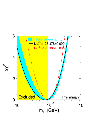
Figure 9: The $\chi^{2}$ distribution as function of the Higgs mass from the SM fit to the electroweak precision observables and the top mass. The shaded area is excluded by the direct searches.

Within the Standard Model the value of the Higgs mass $m_{h}$ is not predicted. However, one can get the bounds on the Higgs mass [31, 32]. They follow from the behaviour of the quartic coupling which obeys the RG equation (1.14).

Since the quartic coupling grows with rising energy indefinitely, an upper bound on $m_{h}$ follows from the requirement that the theory be valid up to the scale $M_{Planck}$ or up to a given cut-off scale $\Lambda$ below $M_{Planck}$ [31]. The scale $\Lambda$ could be identified with the scale at which a Landau pole develops. The upper bound on $m_{h}$ depends mildly on the top-quark mass through the impact of the top-quark Yukawa coupling on the running of the quartic coupling $\lambda$.

On the other hand, the requirement of vacuum stability in the SM (positivity of $\lambda$) imposes a lower bound on the Higgs boson mass, which crucially depends on the top-quark mass as well as on the cut-off $\Lambda$ [31, 32]. Again, the dependence of this lower bound on $m_{t}$ is due to the effect of the top-quark Yukawa coupling on the quartic coupling in eq.(1.14), which drives $\lambda$ to negative values at large scales, thus destabilizing the standard electroweak vacuum.

From the point of view of LEP and Tevatron physics, the upper bound on the SM Higgs boson mass does not pose any relevant restriction. The lower bound on $m_{h}$, instead, is particularly important in view of search for the Higgs boson at LEPII and Tevatron. For $m_{t}\sim 174$ GeV and $\alpha_{s}(M_{Z})=0.118$ the results at $\Lambda=10^{19}$ GeV or at $\Lambda=1$ TeV can be given by the approximate formulae [32]

$$m_{h} > 135+2.1[m_{t}-174]-4.5\left[\frac{\alpha_{s}(M_{Z})-0.118}{0.006}\right],\ \ \ \ \Lambda=10^{19}\ GeV,$$ (7.2)

$$m_{h} > 72+0.9[m_{t}-174]-1.0\left[\frac{\alpha_{s}(M_{Z})-0.118}{0.006}\right],\ \ \ \ \Lambda=1\ TeV,$$ (7.3)

where the masses are in units of GeV.

Fig.10 [45] shows the perturbativity and stability bounds on the Higgs boson mass of the SM for different values of the cut-off $\Lambda$ at which new physics is expected.

Figure 10: Strong interaction and stability bounds on the SM Higgs boson mass. $\Lambda$ denotes the energy scale up to which the SM is valid.

We see from Fig.10 and eqs.(7.2,7.3) that indeed for $m_{t}\sim 174$ GeV the discovery of a Higgs particle at LEPII would imply that the Standard Model breaks down at a scale $\Lambda$ well below $M_{GUT}$ or $M_{Planck}$, smaller for lighter Higgs. Actually, if the SM is valid up to $\Lambda\sim M_{GUT}$ or $M_{Planck}$, for $m_{t}\sim 174$ GeV only a small range of values is allowed: $134<m_{h}<\sim 200$ GeV. For $m_{t}$ = 174 GeV and $m_{h}<100$ GeV [i.e. in the LEPII range] new physics should appear below the scale $\Lambda\sim$ a few to 100 TeV. The dependence on the top-quark mass however is noticeable. A lower value, $m_{t}\simeq$ 170 GeV, would relax the previous requirement to $\Lambda\sim 10^{3}$ TeV, while a heavier value $m_{t}\simeq$ 180 GeV would demand new physics at an energy scale as low as 10 TeV.

7.2 The Higgs boson mass in the MSSM

It has been already mentioned that in the MSSM the mass of the lightest Higgs boson is predicted to be less than the $Z$-boson mass. This is, however, the tree level result and the masses acquire the radiative corrections.

With account of the radiative corrections the effective Higgs bosons potential is

$$V_{Higgs}^{eff}=V_{tree}+\Delta V,$$ (7.4)

where $V_{tree}$ is given by eq.(3.14) and in one loop order

$$\Delta V_{1loop}=\sum_{k}\frac{1}{64\pi^{2}}(-1)^{J_{k}}(2J_{k}+1)c_{k}m_{k}^{4}\left(\log\frac{m_{k}^{2}}{Q^{2}}-\frac{3}{2}\right).$$ (7.5)

Here the sum is taken over all the particles in the loop, $J_{k}$ is the spin and $m_{k}$ is the field dependent mass of a particle at the scale $Q$. These radiative corrections vanish when supersymmetry is not broken and are positive in softly broken case. The leading contribution comes from (s)top loops

$$\Delta V_{1loop}^{stop}=\frac{3}{32\pi^{2}}\left[\tilde{m}_{t_{1}}^{4}(\log\frac{\tilde{m}_{t_{1}}^{2}}{Q^{2}}-\frac{3}{2})+\tilde{m}_{t_{2}}^{4}(\log\frac{\tilde{m}_{t_{2}}^{2}}{Q^{2}}-\frac{3}{2})-2m_{t}^{4}(\log\frac{m_{t}^{2}}{Q^{2}}-\frac{3}{2})\right].$$ (7.6)

Contributions from the other particles are much smaller [46, 47, 48].

These corrections lead to the following modification of the tree level relation for the lightest Higgs mass

$$m_{h}^{2}\approx M_{Z}^{2}\cos^{2}2\beta+\frac{3g^{2}m_{t}^{4}}{16\pi^{2}M_{W}^{2}}\log\frac{\tilde{m}_{t_{1}}^{2}\tilde{m}_{t_{2}}^{2}}{m_{t}^{4}}.$$ (7.7)

One finds that the one loop correction is positive and increases the mass value. Two loop corrections have the opposite effect but are smaller and result in slightly lower value of the Higgs mass.

To find out numerical values of these corrections one has to determine the masses of all superpartners. This means that one has to know the initial conditions for the soft papameters. Fortunately due to the IRQFP solutions the dependence on initial conditions may disappear at low energies. This allows one to reduce the number of unknown parameters and make predictions.

Due to extreme importance of the Higgs mass predictions for experimental searches this problem has been the subject of intense investigation. There is a considerable amount of papers devoted to this topic (see e.g. [47, 48, 49, 52, 57, 60]). And though the initial assumptions and the strategy are different, the general conclusions are very similar.

In what follows we accept the strategy advocated in Refs. [36, 42]: As input parameters one takes the known values of the top-quark, bottom-quark and $\tau$-lepton masses, the experimental values of the gauge couplings, and the mass of the Z-boson [1]. To reduce the arbitrariness of the soft terms we use the fixed-point values for the Yukawa couplings and SUSY breaking parameters. The value of $\tan\beta$ is determined from the relations between the running quark masses and the Higgs v.e.v.’s in the MSSM

$$m_{t} = y_{t}\ v\ \sin\beta\,,$$ (7.8)

$$m_{b} = y_{b}\ v\ \cos\beta\,,$$ (7.9)

$$m_{\tau} = y_{\tau}\ v\ \cos\beta\,.$$ (7.10)

The Higgs mixing parameter $\mu$ is defined from the minimization conditions for the Higgs potential and requirement of radiative EWSB.

As an output we determine the mass spectrum of superpartners and of the Higgs bosons as functions of the only free parameter, namely $m_{1/2}$, which is directly related to the gluino mass $M_{3}$. Varying this parameter within the experimentally allowed range, one gets all the masses as functions of this parameter (see Table2).

INPUT		OUTPUT
$m_{t}(pole)=173.8\pm 5.2$ GeV		$Y_{t},Y_{b},Y_{\tau}$
$m_{b}(pole)=4.94\pm 0.15$ GeV		$A_{t},A_{b},A_{\tau}$
$m_{\tau}(pole)=1.7771\pm 0.0005$ GeV		$\tan\beta,\mu$
$\alpha_{3}(M_{Z})=0.118\pm 0.005$	$\Rightarrow$	$\tilde{m}^{2}_{Q},\tilde{m}^{2}_{U},\tilde{m}^{2}_{D}$
$\alpha_{2}(M_{Z})=0.034$		$\tilde{m}^{2}_{L},\tilde{m}^{2}_{E}$
$\alpha_{1}(M_{Z})=0.017$		$m^{2}_{H_{1}},m^{2}_{H_{2}}$
$M_{Z}=91.187\pm 0.007$ GeV		$m_{h},m_{A},m_{H},m_{H}^{\pm}$

Table 2: The values of input parameters and the output of fixed point analysis

For low $tan\beta$ the value of $\sin\beta$ is determined from eq.(7.8), while for high $\tan\beta$ it is more convenient to use the relation $\tan\beta=\frac{m_{t}}{m_{b}}\frac{y_{b}}{y_{t}}$, since the ratio $y_{t}/y_{b}$ is almost a constant in the range of possible values of $y_{t}$ and $y_{b}$.

For the evaluation of $\tan\beta$ one first needs to determine the running top- and bottom-quark masses. One can find them using the well-known relations to the pole masses (see e.g. [50, 51, 52]), including both QCD and SUSY corrections. For the top-quark one has:

$$m_{t}(m_{t})=\frac{m_{t}^{pole}}{1+\left(\frac{\Delta m_{t}}{m_{t}}\right)_{QCD}+\left(\frac{\Delta m_{t}}{m_{t}}\right)_{SUSY}}\ .$$ (7.11)

Then, the following procedure is used to evaluate the running top mass. First, only the QCD correction is taken into account and $m_{t}(m_{t})$ is found in the first approximation. This allows one to determine both the stop masses and the stop mixing angle. Next, having at hand the stop and gluino masses, one takes into account the stop/gluino corrections.

For the bottom quark the situation is more complicated because the mass of the bottom quark $m_{b}$ is essentially smaller than the scale $M_{Z}$ and so one has to take into account the running of this mass from the scale $m_{b}$ to the scale $M_{Z}$. The procedure is the following [51, 53, 54]: one starts with the bottom-quark pole mass, $m_{b}^{pole}=4.94\pm 0.15$ [55] and finds the SM bottom-quark mass at the scale $m_{b}$ using the two-loop $QCD$ corrections

$$m_{b}(m_{b})^{SM}=\frac{m_{b}^{pole}}{1+\left(\frac{\Delta m_{b}}{m_{b}}\right)_{QCD}}\,.$$ (7.12)

Then, evolving this mass to the scale $M_{Z}$ and using a numerical solution of the two-loop SM RGEs [51, 54] with $\alpha_{3}(M_{Z})=0.12$ one obtains $m_{b}(M_{Z})_{SM}=2.91$ GeV. Using this value one can calculate the sbottom masses and then return back to take into account the SUSY corrections from massive SUSY particles

$$m_{b}(M_{Z})=\frac{m_{b}(M_{Z})^{SM}}{1+\left(\frac{\Delta m_{b}}{m_{b}}\right)_{SUSY}}\,.$$ (7.13)

When calculating the stop and sbottom masses one needs to know the Higgs mixing parameter $\mu$. For determination of this parameter one uses the relation between the $Z$-boson mass and the low-energy values of $m_{H_{1}}^{2}$ and $m_{H_{2}}^{2}$ which comes from the minimization of the Higgs potential:

$$\frac{M_{Z}^{2}}{2}+\mu^{2}=\frac{m_{H_{1}}^{2}+\Sigma_{1}-(m_{H_{2}}^{2}+\Sigma_{2})\tan^{2}\beta}{\tan^{2}\beta-1}\,,$$ (7.14)

where $\Sigma_{1}$ and $\Sigma_{2}$ are the radiative corrections [47]. Large contributions to these functions come from stops and sbottoms. This equation allows one to obtain the absolute value of $\mu$, the sign of $\mu$ remains a free parameter.

Whence the quark running masses and the $\mu$ parameter are found, one can determine the corresponding values of $\tan\beta$ with the help of eqs.(7.8,7.9). This gives in low and high $\tan\beta$ cases, respectively [36, 42, 56]

$$\tan{\beta} = 1.47\pm 0.15\pm 0.05\ \ \ for\ \mu>0\,,$$

$$\tan{\beta} = 1.56\pm 0.15\pm 0.05\ \ \ for\ \mu<0\,,$$

$$\tan{\beta} = 69.3\pm 0.6\pm 0.3\ \ \ \ \ for\ \mu>0\,,$$

$$\tan{\beta} = 38.1\pm 0.9\pm 0.4\ \ \ \ \ for\ \mu<0\,.$$

The deviations from the central value are connected with the experimental uncertainties of the top-quark mass, $\alpha_{3}(M_{Z})$ and uncertainty due to the fixed point values of $y_{t}(M_{Z})$ and $y_{b}(M_{Z})$.

Having all the relevant parameters at hand it is possible to estimate the masses of the Higgs bosons. With the fixed point behaviour the only dependence left is on $m_{1/2}$ or the gluino mass $M_{3}$. It is restricted only experimentally: $M_{3}>144$ GeV [43] for arbitrary values of the squarks masses.

Let us start with low $\tan\beta$ case. The masses of CP-odd, charged and CP-even heavy Higgses increase almost linearly with $M_{3}$. The main restriction comes from the experimental limit on the lightest Higgs boson mass. It excludes $\mu<0$ case and for $\mu>0$ requires the heavy gluino mass $M_{3}\geq 750$ GeV. Subsequently one obtains [36]

$$m_{A}>844\ GeV,\ \ m_{H^{\pm}}>846\ GeV,\ \ m_{H}>848\ GeV,\ \ \ for\ \mu>0,$$

i.e. these particles are too heavy to be detected in the nearest experiments.

For high $\tan\beta$ already the requirement of positivity of $m_{A}^{2}$ excludes the region with small $M_{3}$. In the most promising region $M_{3}>1$ TeV ($m_{1/2}>300$ GeV) for the both cases $\mu>0$ and $\mu<0$ the masses of CP-odd, charged and CP-even heavy Higgses are also too heavy to be detected in the near future [42]

$$m_{A}>1100\ \mbox{GeV for}\ \ \mu>0,\ \ \ m_{A}>570\ \mbox{GeV for}\ \ \mu<0,$$

$$m_{H^{\pm}}>1105\ \mbox{GeV for}\ \ \mu>0,\ \ \ m_{H^{\pm}}>575\ \mbox{GeV for}\ \ \mu<0.$$

$$m_{H}>1100\ \mbox{GeV for}\ \ \mu>0,\ \ \ m_{H}>570\ \mbox{GeV for}\ \ \mu<0.$$

The situation is different for the lightest Higgs boson $h$, which is much lighter. Radiative corrections in this case are crucial and increase the value of the Higgs mass substantially [48, 47]. They have been calculated up to the second loop order [58, 60]. As can be seen from eq.(7.7) the one loop correction is positive increasing the tree level value almost up to 100% and the second one is negative thus decreasing it a little bit. We use in our analysis the leading two-loop contributions evaluated in ref.[48]. As has been already mentioned these corrections depend on the masses of squarks and the other superpartners for which we substitute the values obtained above from the IRQFP’s.

The results depend on the sign of parameter $\mu$. It is not fixed since the requirement of EWSB defines only the value of $\mu^{2}$. However, for low $\tan\beta$ negative values of $\mu$ lead to a very small Higgs mass which is already excluded by modern experimental data, so further on we consider only the positive values of $\mu$. Fot high $\tan\beta$ both signs of $\mu$ are allowed.

Consider first the low $\tan\beta$ regime. At the upper part of Fig.11 it is shown the value of $m_{h}$ for $\mu>0$ as a function of the geometrical mean of stop masses - this parameter is often identified with a supersymmetry breaking scale $M_{SUSY}$. One can see that the value of $m_{h}$ quickly saturates close to $\sim$ 100 GeV. For $M_{SUSY}$ of the order of 1 TeV the value of the lightest Higgs mass is [36]

$$m_{h}=(94.3+1.6+0.6\pm 5\pm 0.4)\ \mbox{GeV},\ \ \ \mbox{ for}\ M_{SUSY}=1\ TeV,$$ (7.15)

where the first uncertainty comes from the deviations from the IRQFPs for the mass parameters, the second one is related to that of the top-quark Yukawa coupling, the third reflects the uncertainty of the top-quark mass of 5 GeV, and the last one comes from that of the strong coupling.

One can see that the main source of uncertainty is the experimental error in the top-quark mass. As for the uncertainties connected with the fixed points, they give much smaller errors of the order of 1 GeV.

The obtained result (7.15) is very close to the upper boundary, $m_{h}=97$ GeV, obtained in Refs. [52, 57]. Note, however, that the uncertainties mentioned above as well as the upper bound [52, 57] are valid for the universal boundary conditions. Loosing these requirement leads to increase of the upper bound values of the Higgs mass in case of low $\tan\beta$ up to $\sim 102$ GeV [59].

For the high $\tan\beta$ case the lightest Higgs is slightly heavier, but the difference is crucial for LEP II. The mass of the lightest Higgs boson as a function of $M_{SUSY}$ is shown in the lower part of Fig.11 . One has the following values of $m_{h}$ at a typical scale $M_{SUSY}=1$ TeV ($M_{3}\approx 1.3$TeV) [42]:

$$m_{h} = 128.2-0.4-7.1\pm 5\ \mbox{GeV, \ for}\ \mu>0\,,$$

$$m_{h} = 120.6-0.1-3.8\pm 5\ \mbox{GeV,\ for}\ \mu<0\,.$$

The first uncertainty is connected with the deviations from the IRQFPs for mass parameters, the second one with the Yukawa coupling IRQFPs, and the third one is due to the experimental uncertainty in the top-quark mass. One can immediately see that the deviations from the IRQFPs for mass parameters are negligible and only influence the steep fall of the function on the left, which is related to the restriction on the CP-odd Higgs boson mass $m_{A}$. In contrast with the low $\tan\beta$ case, where the dependence on the deviations from Yukawa fixed points was about $1$ GeV, in the present case it is much stronger. The experimental uncertainty in the strong coupling constant $\alpha_{s}$ is not included because it is negligible compared to those of the top-quark mass and the Yukawa couplings and is not essential here contrary to the low $\tan\beta$ case.

One can see that for large $\tan\beta$ the masses of the lightest Higgs boson are typically around 120 GeV that is too heavy for observation at LEP II. Note, however, that the uncertainties increase if one considers the non-universal boundary conditions which decreases the lower boundary for the Higss mass. At the same time recent experimental data has practically excluded the low $\tan\beta$ scenario and in the next year the situation will be completely clarified.

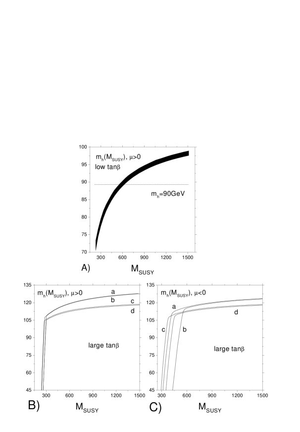
Figure 11: A) The dependence of the mass of the lightest Higgs boson $h$ on $M_{SUSY}=(\tilde{m}_{t_{1}}\tilde{m}_{t_{2}})^{1/2}$ (shaded area) for $\mu>0$, low $\tan\beta$. The dashed line corresponds to the minimum value of $m_{h}=90$ GeV allowed by experiment. B),C) The mass of the lightest Higgs boson $h$ as function of $M_{SUSY}$ for different signs of $\mu$, large $\tan\beta$. The curves (a,b) correspond to the upper limit of the Yukawa couplings and to $m_{0}^{2}/m_{1/2}^{2}=0$ (a) or to $m_{0}^{2}/m_{1/2}^{2}=2$ (b). The curves (c,d) correspond to the lower limit of the Yukawa couplings and to $m_{0}^{2}/m_{1/2}^{2}=0$ (c) or to $m_{0}^{2}/m_{1/2}^{2}=2$ (d). Possible values of the mass of the lightest Higgs boson are inside the areas marked by these lines.

Thus, one can see that in the IRQFP approach all the Higgs bosons except for the lightest one are found to be too heavy to be accessible in the nearest experiments. This conclusion essentially coincides with the results of more sophisticated analyses. The lightest neutral Higgs boson, on the contrary is always light. The situation may improve a bit if one considers more complicated models with enlarged Higgs structure [61]. However, it does not change the generic feature of SUSY theories, the presence of light Higgs boson.

In the near future with the operation of the Tevatron and LHC proton-antiproton accelerators with the c.m energy of 2 and 15 TeV, respectively, the energy range from 100 to 1000 GeV will be scanned and supersymmetry will be either discovered or the minimal version will be abandoned in particle physics. The Higgs boson might be the first target in search of SUSY.

8 Conclusion

We have attempted to show how following the pattern of RG flow one can explore physics lying beyond the Standard Model of fundamental interactions. The methods are essentially based on renormalization group technique in the framework of quantum field theory. The running of parameters is the key ingredient in attempts to go beyond the range of energies accessible to modern accelerators, to find manifestation of new physics. In the absence of solid experimental facts the RG flow happens to be the only sauce of definite predictions. The peculiarity of the moment is that these predictions are the subject of experimental tests today, and in the near future, so one may hope to check the ideas described above at the turn of the Millennium.

Acknowledgments

The author is grateful to S.Codoban, A.Gladyshev, M.Jurčišin, V.Velizhanin, K.Ter-Martirossian, R.Nevzorov, W. de Boer and G.Moultaka for useful discussions and to S.Codoban for help in preparing the manuscript. Special thanks to the organizers of the conference D.O’Connor and C.Stephens. Financial support from RFBR grants # 99-02-16650 and # 96-15-96030 is kindly acknowledged.

References

- [1] Review of Particle Properties. European Physics J. C3 (1998).
- [2] Reports of the Working group on Precision calculations for the Z-resonance, CERN Yellow Report, CERN 95-03, eds D.Bardin, W.hollik and G.Passarino.
- [3] see e.g. B.Pendelton and G.G.Ross, Phys.Lett B98 (1981) 291.
- [4] The LEP Collaborations: ALEPH, DELPHI, L3 and OPAL and the LEP electroweak Working Group;. Phys. Lett. 276B (1992) 247;. Updates are given in CERN/PPE/93-157, CERN/PPE/94-187 and LEPEWWG/95-01 (see also ALEPH 95-038, DELPHI 95-37, L3 Note 1736 and OPAL TN284.
- [5] G. G. Ross, Grand Unified Theories, (Benjamin Cummings, 1985).
- [6] Y.A.Golfand and E.P.Likhtman, JETP Letters, 13 (1971) 452; D.V.Volkov and V.P.Akulov, JETP Letters, 16 (1972) 621; J.Wess and B.Zumino, Phys.Lett., B49 (1974) 52.
- [7] S.Coleman and J.Mandula, Phys.Rev., 159 (1967) 1251.
- [8] P. West, Introduction to Supersymmetry and Supergravity, (World Scientific, 1986),
- [9] S.J.Gates, M.Grisaru, M.Roček and W.Siegel, Superspace or One Thousand and One Lessons in Supersymmetry, Benjamin/ Cummings, 1983.
- [10] J. Wess and J. Bagger, Supersymmetry and Supergravity, (Princeton University Press, 1983)
- [11] F.A.Berezin, The Method of Second Quantization, Moscow, Nauka, 1965.
-
[12]
P. Fayet and S. Ferrara, Phys. Rep. 32 (1977) 249
M. F. Sohnius, Phys. Rep. 128 (1985) 41.
H. P. Nilles, Phys. Rep. 110 (1984) 1,
H. E. Haber and G. L. Kane, Phys. Rep. 117 (1985) 75.
A.B.Lahanas and D.V. Nanopoulos, Phys. Rep. 145 (1987) 1;
R. Barbieri, Riv. Nuo. Cim. 11 (1988) 1;
W. de Boer, Progr. in Nucl. and Particle Phys., 33 (1994) 201;
D.I. Kazakov, Surveys in High Energy Physics, 10 (1997) 153. - [13] H. E. Haber, Introductory Low-Energy Supersymmetry, Lectures given at TASI 1992, (SCIPP 92/33, 1993).
- [14] J. Gunion, H. Haber, G. Kane and S. Dawson, Higgs Hunter’s Guide, (Addison-Wesley, New York, 1990).
- [15] P. Fayet, Phys. Lett. B69 (1977) 489; G. Farrar and P. Fayet, Phys. Lett. B76 (1978) 575.
- [16] H. Dreiner and G. G. Ross, Nucl. Phys. B365 (1991) 597, K. Enqvist, A. Masiero and A. Riotto, Nucl. Phys. B373 (1992) 95,
-
[17]
L. Hall, J. Lykken and S. Weinberg, Phys. Rev. D27
(1987) 2359;
S. K. Soni and H.A. Weldon, Phys. Lett. B126 (1983) 215. - [18] A. H. Chamseddine, R. Arnowitt and P. Nath, Phys.Rev.Lett. 49 (1982) 970; R. Barbieri, S. Ferrara and C. A. Savoy, Phys.Lett. B119 (1982) 343; L. Hall, J. Lykken and S. Weinberg, Phys.Rev., D27 (1983) 2359.
- [19] N. Polonsky and A. Pomarol, Phys. Rev. Lett. 73 (1994) 2292; Phys. Rev. D51 (1995) 6532.
-
[20]
G. G. Ross and R. G. Roberts, Nucl. Phys. B377
(1992) 571.
V. Barger, M. S. Berger and P. Ohmann, Phys. Rev. D47 (1993) 1093.
W. de Boer, R. Ehret and D. Kazakov, Z. Phys. C67 (1995) 647 ; W.de Boer, et al., Z.Phys. C71 (1996) 415. - [21] U. Amaldi, W. de Boer and H. Fürstenau, Phys.Lett. B260 (1991) 447.
- [22] P. Langaker and M. Luo, Phys.Rev. D44 (1991) 817.
- [23] J. Ellis, S. Kelley and D. V. Nanopoulos, Nucl.Phys. B373 (1992) 55.
- [24] I. Antoniadis, C. Kounnas, and K. Tamvakis, Phys. Lett. 119B (1982) 377.
- [25] Y.Yamada, Phys.Rev., D50 (1994) 3537.
- [26] I.Jack and D.R.T.Jones, Phys.Lett. B415 (1997) 383, hep-ph/9709364.
- [27] L.A.Avdeev, D.I.Kazakov and I.N.Kondrashuk, Nucl.Phys. B510 (1998) 289, ( hep-ph/9709397).
- [28] G. Giudice and R. Rattazzi, Nucl. Phys. B511 (1998). 25.
- [29] D.I. Kazakov, Proceedings of XXIX ICHEP’98 Conference, Vancouver, 1999, p.1590.
- [30] D.I. Kazakov, Phys.Lett. B449 (1999) 201, hep-ph/9812513.
-
[31]
N.Cabibbo, L.Maiani, G.Parisi, and R.Petronzio, Nucl. Phys. B158
(1979) 295;
M.Lindner, Z.Phys. C31 (1986) 295; M.Sher, Phys.Rev. D 179 (1989) 273; M.Lindner, M.Sher and H.W.Zaglauer, Phys.Lett. B228 (1989) 139. -
[32]
M.Sher, Phys.Lett. B317 (1993) 159; C.Ford,
D.R.T.Jones, P.W.Stephenson and M.B.Einhorn, Nucl.Phys. B395
(1993) 17;
G.Altarelli and I. Isidori, Phys.Lett. B337 (1994) 141; J.A.Casas, J.R.Espinosa and M.Quiros, Phys.Lett. 342 (1995) 171. -
[33]
C. T. Hill, Phys. Rev. D24 (1981) 691,
C. T. Hill, C. N. Leung and S. Rao, Nucl. Phys. B262 (1985) 517. - [34] L.E.Ibáñez, C.Lopéz and C.Muñoz, Nucl.Phys. B256 (1985) 218.
-
[35]
P.Langacker, N.Polonsky, Phys.Rev. D49 (1994)
454
M.Carena et al, Nucl.Phys. B419 (1994) 213
M.Carena, C.E.M.Wagner, Nucl.Phys. B452 (1995) 45.
M.Lanzagorta, G.Ross, Phys. Lett. B364 (1995) 163.
J. Feng, N. Polonsky and S. Thomas, Phys. Lett. B370 (1996) 95,
N. Polonsky, Phys. Rev. D54 (1996) 4537. - [36] G.K.Yeghiyan, M.Jurčišin and D.I.Kazakov, Mod. Phys.Lett . A14 (1999) 601, hep-ph/9807411.
- [37] I.Jack and D.R.T.Jones, Phys. Lett. B443 (1998) 117, hep-ph/9809250.
- [38] S. Codoban and D.I. Kazakov, hep-ph/9906256, to appear in Eur.Phys.J. C.
- [39] S.A.Abel, B.C.Allanach, Phys. Lett. B415 (1997) 371.
- [40] G. Auberson and G. Moultaka, hep-ph/9907204, to appear in Eur.Phys.J. C.
- [41] D.Kazakov amd G.Moultaka, hep-ph/9912271.
- [42] M.Jurčišin and D.I.Kazakov, Mod. Phys.Lett. A14 (1999) 671, hep-ph/9902290.
-
[43]
LEP Electroweak Working Group, CERN-EP/99-15, 1999,
http://www.cern.ch/LEPEWWG/lepewpage.html.
V.A.Novikov, L.B.Okun, A.N.Rozanov and M.I. Vysotsky, LEPTOP, Reports on Progress in Physics 62 (1999) 1275. - [44] see e.g. http://alephwww.cern.ch : A.Blondel talk at LEPC, Nov.1999.
- [45] T.Hambye, K.Reisselmann, Phys.Rev. D55 (1997) 7255; H.Dreiner, hep-ph/9902347.
- [46] J. Ellis, G. Ridolfi, F. Zwirner, Phys.Lett B262 (1991) 477; A. Brignole, J. Ellis, G. Ridolfi, F. Zwirner, Phys.Lett 271 (1991) 123.
- [47] A.V.Gladyshev, D.I.Kazakov, W.de Boer, G.Burkart and R.Ehret, Nucl. Phys. B498 (1997) 3.
-
[48]
M.Carena, J.R.Espinosa, M.Quiros and C.E.M.Wagner, Phys.Lett.
B355 (1995) 209;
J.Ellis, G.L.Fogli and E.Lisi, Phys.Lett B333 (1994) 118 - [49] H.Haber and R.Hempfling, Phys.Rev.Lett. 66 91991) 1815; Y.Okada, M.Yamaguchi and T.Yanagida, Prog.Theor.Phys. 85 (1991)1; J.Ellis, G.Rudolfi and F.Zwirner, Phys.Lett. B257 (1991) 83; ibid B262 (1991) 477; R.Barbieri and M.Frigeni, Phys.Lett. B258 (1991) 305; P.Chankowski, S.Pokorski and J.Rosiek, Nucl.Phys. B423 (1994) 437; A.Dabelstein, Nucl.Phys. B456 (1995) 25; Z.Phys. C67 (1997)3.
- [50] B.Schrempp, M.Wimmer, Prog.Part.Nucl.Phys. 37 (1996) 1.
-
[51]
D.M.Pierce, J.A.Bagger, K.Matchev and R.Zhang, Nucl.Phys. B491 (1997) 3,
J.A.Bagger, K.Matchev and D.M.Pierce, Phys.Lett. B348 (1995) 443. - [52] J.Casas, J.Espinosa, H.Haber, Nucl.Phys. B526 (1998)3.
- [53] H.Arason, D.Castano, B.Keszthelyi, S.Mikaelian, E.Piard, P.Ramond, and B.Wright, Phys.Rev. D46 (1992) 3945.
- [54] N.Gray, D.J.Broadhurst, W.Grafe, and K.Schilcher, Z.Phys. C48 (1990) 673.
- [55] C.T.H.Davies, et al., Phys.Rev. D50 (1994) 6963.
- [56] D.I.Kazakov, in ”Why Matter Matters?”, Phys. Rep. 320 (1999) 187, (hep-ph/9905330).
- [57] W.de Boer, H.-J.Grimm, A.V.Gladyshev and D.I.Kazakov, Phys.Lett. B438 (1998) 281.
- [58] H.Haber, R.Hempfling and A.Hoang, Z.Phys. C75 (1997) 539 R.Hempfling and A.Hoang, Phys.Lett. B331 (1994) 99. R. Hempfling, Phys. Rev. D49 (1994) 6168.
- [59] S.Codoban, M.Jurčišin and D.Kazakov, to appear.
- [60] S. Heinemeyer, W. Hollik and G. Weiglein, Phys. Lett. B455 (1999) 179, (hep-ph/9903404 ); Eur. Phys. J. C9 (1999) 343, (hep-ph/9812472).
- [61] M.Masip, R.Muñoz-Tapia and A.Pomarol, Phys.Rev. D57 (1998) 5340.