Overview of Chiral Perturbation Theory
Abstract
I present a quick overview of the current status of Chiral perturbation theory in the meson sector. To illustrate the successes and some problems in the description of the phenomenology, I focus on a few selected examples that are relevant for DANE.
1 Introduction
Chiral perturbation theory (CHPT) is the low–energy effective theory of the strong interactions. To characterise quantitatively the meaning of “low energy” in this framework, we recall that the relevant physical scale here is that of spontaneous chiral symmetry breaking, i.e. about 1 GeV: the effective theory is supposed to work only for GeV. For practical purposes one expects CHPT to work reasonably well up to 500–600 MeV. Which means that at DANE, as soon as the decays we enter the realm of CHPT: for any physical process occurring after the decay of the there is most likely some relevant piece of information that can be derived from CHPT (a check on this claim can be easily made by glancing through the “Second DANE Physics Handbook”[1]).
This effective field theory is a systematic extension of the current–algebra methods that were used in the sixties in hadronic physics. Its present form is due to Weinberg[2] and Gasser and Leutwyler[3]. They showed the advantages of the effective–field–theory language over the direct implementation of the Ward identities as in the current–algebra framework. In particular because what was known before as a tremendously difficult problem, the calculation of the corrections to a current–algebra result, was reduced to a routine loop calculation in a well–defined framework. After the convenient tools of the effective field theory were made available, many processes have been calculated at the one–loop level: wherever possible, the comparison to the experimental data has shown a remarkable success of the method.
In the early nineties, also because of the prospects of having a –factory operating soon, the first two–loop calculations were made. The first one was the cross section for the two–photon annihilation into two neutral pions[4]. This beautiful and difficult calculation opened up the field of two–loop calculations in CHPT. In fact if we consider only the two–light–flavour sector, all the phenomenologically relevant calculations have already been done, whereas in the framework, they are just starting[5]. Moreover, in the purely strong sector, the Lagrangian at order and the complete divergence structure have been recently calculated[6]. What I find remarkable is that, despite the rapidly increasing number of new constants appearing at each new order[3, 6], the theory is able to produce sharp predictions, like in the first instance, the calculation of the cross section. The best illustration of this is the scattering reaction, that I will discuss in more details in the following section.
In parallel to these two–loop calculations arose the need to account for small effects such as electromagnetic corrections and purely strong isospin–breaking effects. While the latter are readily calculated with the Lagrangian of Gasser and Leutwyler, the former need the inclusion of the electromagnetic field in the theory. Loops with a virtual photon field generate new types of divergences, that need new counterterms to be removed. Such a Lagrangian was formulated by Urech, and Neufeld and Rupertsberger[7] at order for the strong sector. For processes involving also leptons one needs a further extension of the Lagrangian to account for contributions of virtual leptons inside the loops. This has been formulated only very recently[8], opening up the way to phenomenological applications, such as semileptonic kaon decays. This is an essential step forward if we want to fully exploit the precision of the data on decays that experimentalists are starting to provide[9, 10].
The application of CHPT to weak nonleptonic decays is more problematic because of the presence of more constants already at order . In addition, there are less measured quantities from which to extract these constants. This means, e.g., that in the classical sector of the kaon decays into two or three pions CHPT has rather little to say (recently there has been a very nice counterexample[11] to this statement). The situation improves if one looks at the radiative–nonleptonic–decay sector, where the theory can make predictions ands can be meaningfully tested. I will discuss this topic in Sect. 3.
Conceptually, the basic ingredients in the formulation of CHPT are the spontaneous (global) symmetry breaking and the existence of a mass gap in the spectrum between the Goldstone modes and the other energy levels. The effective field theory for such a situation can be formulated in very general terms, without any reference to a specific symmetry group, or a specific physical system. This method has in fact been applied to a variety of different physical systems and situations, ranging from solid–state systems to strong interactions at finite temperature and volume, to QCD in the quenched approximation, etc. I will not discuss these different fields of applications (I refer the interested reader to the excellent reviews available in the literature [12]), and restrict myself to applications in the meson sector only, leaving out also the very important and rich field of baryon physics.
2 Phenomenological applications: strong sector
Phenomenological applications in the strong sector are nowadays at the level of two–loop calculations. scattering[13] is the best example to show what high level of precision one can aim to with two–loop CHPT. The scattering lengths, predicted in CHPT, can be measured in decays, but also with the help of pionic atoms. It is known since many years that the lifetime of pionic atoms is proportional to the square of the difference of the two –wave scattering lengths, modulo corrections. A precise evaluation of these corrections is crucial if one wants to pin down the scattering lengths at a few percent level. CHPT can help also in this case. It is a beautiful example of the power of the method, which also shows that the field is still open to progress at the methodological level, not only via multiloop calculations.
2.1 scattering
This is the “golden reaction” for Chiral Perturbation Theory: at threshold the naive expansion parameter is , and already a tree level calculation[14] should be rather accurate. This rule of thumb is quite misleading here, as it is shown by the fact that both the one–loop[15] and the two–loop[13] calculations produced substantial corrections. The violation of the rule of thumb has a well known origin, and is due to the presence of chiral logarithms , which, for GeV change the expansion parameter by a factor four. If we look at the –wave scattering lengths, e.g., a large coefficient in front of the single (at one loop) and double (at two loops) chiral logarithms is the main source of the large correction[15, 16]:
| (1) | |||||
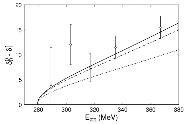
The same picture is maintained if we move away from threshold. In Fig. 1 one can see the comparison of the three successive chiral orders and the experimental data for the phase–shift difference coming from decays. The figure shows a well behaved series that ends up in rather good agreement with the experimental data. At this level of accuracy of the experimental data, however, the comparison is not particularly instructive, and even a precise assessment of the theoretical uncertainties would not seem necessary. The real challenge comes from the present generation of experiments: both KLOE at DANE and E865 in Brookhaven[9] will be able to analyse a factor ten more events than the old Geneva–Saclay collaboration[17]. Without taking into account the improvements in the systematics (which should be particularly important for KLOE in view of its very clean environment), the reduction of the error bars is of about a factor three. Which makes it a real precision test.
To make the discussion of the numerics a little simpler it is useful to come back to the scattering length. To compare theory and experiment here we first have to solve the problem of the extraction of the scattering length from the measurement of the phase shift. Can this be done reliably, without introducing further uncontrolled uncertainties? The answer is positive, and the method to do this relies on solving numerically the Roy equations. The latter embody in a rigorous way the analyticity and crossing–symmetry properties of the scattering amplitude – when supplemented with the unitarity relations they become nonlinear, and amenable only to numerical studies. The physical scattering amplitude must obviously satisfy them. These equations have two subtraction constants: the two –wave scattering lengths. If one specifies the values of these two subtraction constants (and also uses experimental input at high energy, ), the solution is unique. One may reverse the argument and say that the physical amplitude away from threshold (as measured experimentally in decays) determines unambiguously the two scattering lengths.
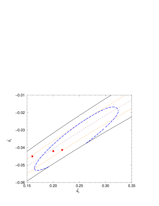
Such a program had been carried out in the seventies by Basdevant, Froggatt and Petersen[18]. Today it has been revived[19] to be used again with the new generation of experimental measurements. Both the new[19] and the old analysis[18] of Roy equations agree in that the data of the Geneva–Saclay collaboration constrain the –wave scattering length to be roughly between and in pion mass units. This can be seen in Fig. 2, where it is shown the 70% C.L. contour as obtained[19] from the analysis of the available experimental data in the low–energy region[17, 20]. The chiral prediction is clearly well compatible, but in principle, a reduction of the range to one third of its present size could show a discrepancy between the experiment and the theory. What would this mean? Could the theory change its numerical estimate by adjusting a few parameters here and there? A necessary ingredient to formulate an answer is a careful estimate of the uncertainties to be attached to the two–loop prediction of CHPT[21]. This careful estimate, however, will say whether the final uncertainty is 3, or 5 or 10%, it is already very clear that there is no way for CHPT to be in agreement with the central (or higher) value of as preferred from the Geneva–Saclay data, .
The only way to understand such a central value is a drastic change of perspective at a very fundamental level: a value of the quark–antiquark condensate much smaller than what we currently believe (and implicitly assume in the formulation of CHPT) would increase substantially, already at tree level, the value of [22]:
| (2) |
2.2 Decay of bound states
An alternative method to measure experimentally the scattering lengths uses pionic atoms, and therefore has the advantage of measuring the interaction of pions right at threshold. The atom is an electromagnetic bound state which decays predominantly into via strong interactions. The leading–order expression for the width reads[23]:
| (3) |
The DIRAC experiment at CERN aims to accurately measure the lifetime of pionic atoms. The goal is a 10% accuracy on the width, i.e. 5% on the scattering lengths. This simple and direct translation of the errors from what is actually measured (the lifetime) to the scattering lengths illustrates the tremendous advantage of the use of pionic atoms. The advantage, however, would be a fake one, if the the leading order expression for the lifetime (3) was subject to large and/or difficult–to–control corrections.
There have been various attempts to calculate the corrections to the formula (3), with several different methods[24]. The results were, unfortunately, not always in mutual agreement, and due to basic differences in the approaches, it seemed difficult to trace the origin of the discrepancies. The situation has now changed, thanks to the calculation of these corrections that was made in the framework of CHPT [25]. The calculation required the combined use of the CHPT Lagrangian and the nonrelativistic Lagrangian method proposed by Caswell and Lepage[26]. The result can be expressed in the following form:
| (4) |
where
| (5) |
| (6) |
where and are counted as small quantities of order . In the formulae above, are meant in the isospin limit and for . The advantage of the use of CHPT is very clear: the method does not only provide a number for the correction to the leading order formula (3), but rather an algebraic expression, a Taylor series expansion in , with coefficients that can be calculated unambiguously. If anybody wants to calculate these corrections with a different method, he should also be able to compare the results for the coefficients, and easily understand the origin of possible differences. One could have in principle a more clever way to calculate these corrections, summing up series of terms to all orders, but possibly not having the complete leading correction: a comparison at the algebraic level would easily clarify all these aspects. This program of detailed comparisons between different methods has in fact already been started. A handy summary of the present status can be found in the MiniProceedings of HadAtom99[24], where the interested reader will also find reference to the relevant literature.
3 Phenomenological applications: weak sector
In the weak–interaction sector the lowest order Lagrangian contains only two constants: and . The situation is therefore similar to the one in the strong sector at this level. At next–to–leading order the Lagrangian contains 37 new constants called the [27]. Such a large number of constants seems to make the situation hopeless. In the sector of decays into two or three pions, one can say that to a large extent it is so. In the sense that it is difficult to make predictions: one does not have enough observables from which to determine some of the relevant constants, at best one can only fit the data. Moreover, the simple method of resonance saturation to estimate the values of the constants, does not seem to work in the weak sector as it does in the strong one. At least not as straightforwardly.
The situation improves if one considers the nonleptonic radiative decays: here only a restricted set of the constants contribute and there are many more observables from which to determine them. In fact KLOE and the fixed target experiments at Brookhaven and Fermilab are going to collect an impressive number of data on many of these decays[9, 10], and will allow to determine rather precisely several of the constants. I will concentrate in what follows on a couple of such decays, discussing the importance of contributions, when the order fails to describe the data at the present level of accuracy. While a complete formulation of the theory (knowledge of the complete Lagrangian and divergence structure) at order in the weak sector is completely out of sight at the moment, it is possible to push the calculation at the level, picking up only the presumably dominant terms.
3.1
Assuming conservation the is determined by two invariant amplitudes, and , , where are the momenta of the two photons, and that of the kaon. At order : . At order [28]: , and , where is a loop function generated by intermediate state in the channel, that represents the dominant effect at this order, and the ellipsis stands for other less important contributions. Although the shape of the spectrum was nicely confirmed by the experiment[30, 31], the branching ratio was a factor three too small:
| (7) |
therefore requiring large corrections. The calculations at order [29] have considered only the (possibly dominant) corrections to the pion loops, and added to this a polynomial contribution:
where and also come from intermediate state in the channel. To get into agreement with the experiment one needed to have a large and negative : with and with . Also for the spectrum, unitarity corrections alone were not sufficient (and actually worsened the agreement), while an improved agreement with the data is obtained only with .
The outcome of this analysis is therefore a clear need for a very large contribution from the polynomial part. Is this reasonable or does it signal a serious failure of the chiral expansion in this case? Another way to formulate this question is to ask whether we understand the dynamical reason to have such a large constant. It is important to give a historical perspective here. In ’93 Cohen, Ecker and Pich in Ref.[28] described the situation as follows: “Several model estimates of have been made in the literature. A fair summary of those attempt is that we know neither the sign nor the magnitude of .” More recently D’Ambrosio and Portolés[32] have built a Vector Resonance Model that does indeed get the right sign and size for this constant: . This number is now in amazing agreement with the one extracted from a fit to the most recent data[33].
Although D’Ambrosio and Portolés estimate of was only a postdiction, it is reassuring to have an understanding of the size of this constant. In fact it is not the only case where one can find this relative size between the various contributions in the chiral expansion. A well–known analogous example in the strong sector is the vector form factor. Its Taylor expansion around is usually defined as . vanishes at order , and can be predicted with no parameters at order . Nowadays it is known up to order [34]:
where the
latter value is determined experimentally. Here also:
i) the order parameter–free prediction fails badly;
ii) there are large unitarity corrections;
iii) but even larger polynomial contributions,
coming from the resonance.
3.2
Already in 1987 Ecker, Pich and de Rafael[35] calculated the amplitude of this decay mode at order . The amplitude depends on one (unknown) low–energy constant. Since we have two leptonic modes we can fix the constant in one of the two and then predict the other. Years after the theoretical prediction data have appeared for both leptonic modes: BNL-E777 on the electron mode[36] and BNL-E787 on the muon mode [37]. There are various interesting aspects in this decay mode, and I refer the interested reader to a recent paper where one can also find reference to the relevant literature[38]. Here I only want to discuss one particular number, the ratio of the width in the two modes. The experimental measurements gave
| (9) |
which is away from the CHPT value . Again an example of a quantity subject to large corrections from higher orders? D’Ambrosio, Ecker, Isidori and Portolés[38] have extended the analysis to include the main effects: unitarity corrections (reliably calculable) and polynomial contributions (estimated with theoretical modelling). Their conclusion is that there is no room for large corrections: . A recent new measurement[39] of the muon mode has brought the experimental number into agreement with the theoretical prediction.
4 Conclusions
Chiral perturbation theory is an essential tool to describe kaon physics, an extremely interesting physics field that continues to have a very deep impact on our knowledge and understanding of the physics of the Standard Model, and also on what lies beyond it. DANE and KLOE, as well as fixed target experiments[9, 10], are now starting to explore this field at a very high precision level. I have quickly reviewed the current status of this effective field theory, with special emphasis on a few physics issues that are relevant for DANE.
In some of the examples I have discussed theory is ahead of experiment, and provides a solid and accurate prediction: the forthcoming experiments will thoroughly test the theory and in particular (in scattering) a very fundamental aspect of the strong interactions, the structure of the chiral symmetry breaking. In other cases experiment is ahead of theory, and is providing essential informations for our understanding of the strong and weak interactions, and their interplay.
Acknowledgements
I warmly thank the organisers for the invitation to such an interesting and successful conference.
References
- 1 . L. Maiani, G. Pancheri and N. Paver (eds.), The Second DANE Physics Handbook (INFN, Frascati, 1995).
- 2 . S. Weinberg, Physica A 96, 327 (1979).
- 3 . J. Gasser and H. Leutwyler, Ann. Phys. (N.Y.) 158, 142 (1984), and Nucl. Phys. B 250, 465 (1985).
- 4 . S. Bellucci, J. Gasser and M. Sainio, Nucl. Phys. B 423, 80 (1994); B 431,413 (1994) (E).
- 5 . G. Amoros, J. Bijnens and P. Talavera, hep-ph/9912398.
- 6 . J. Bijnens, G. Colangelo and G. Ecker, JHEP 9902 020 (1999), hep-ph/9907333, Ann. Phys. (N.Y.), in press.
- 7 . R. Urech Nucl. Phys. B 433, 234 (1995); H. Neufeld and H. Rupertsberger Z. Phys. C71, 131 (1996).
- 8 . M. Knecht, H. Neufeld, H. Rupertsberger, and P. Talavera, hep-ph/9909284.
- 9 . J. Lowe, these proceedings.
- 10 . ; S. Kettell, these proceedings.
- 11 . G. Ecker, G. Müller, H. Neufeld, and A. Pich, hep-ph/9912264
- 12 . J. Bijnens Int. J. Mod. Phys. A8, 3045 (1993); J.F. Donoghue, E. Golowich, B.R. Holstein, “Dynamics of the Standard Model” Cambridge Univ. Pr. (1992); G. Ecker, Prog. Part. Nucl. Phys. 35, 1 (1995); J. Gasser hep-ph/9912548; H. Leutwyler, hep-ph/9406283; A. Pich hep-ph/9806303; E. de Rafael, Boulder TASI 0015 (1994), hep-ph/9502254.
- 13 . J. Bijnens, G. Colangelo, G. Ecker, J. Gasser and M. Sainio, Phys. Lett. B 374, 210 (1996), Nucl. Phys. B 508, 263 (1997).
- 14 . S. Weinberg, Phys. Rev. Lett. 17, 616 (1966).
- 15 . J. Gasser and H. Leutwyler, Phys. Lett. B 125, 325 (1983).
- 16 . G. Colangelo, Phys. Lett. B 350, 85 (1995); B 361, 234 (1995) (E).
- 17 . L. Rosselet et al. Phys. Rev. D 15, 574 (1977).
- 18 . J.L. Basdevant, C.D. Froggatt, and J.L. Petersen, Nucl. Phys. B 72, 413 (1974).
- 19 . B. Ananthanarayan, G. Colangelo, J. Gasser, H. Leutwyler and G. Wanders, work in progress.
- 20 . W. Hoogland et al. Nucl. Phys. B 126, 109 (1977).
- 21 . G. Colangelo, J. Gasser, and H. Leutwyler work in progress.
- 22 . M. Knecht, B. Moussallam, J. Stern and N.H. Fuchs, Nucl. Phys. B 457, 513 (1995).
- 23 . S. Deser, M.L. Goldberger, K. Baumann, and W. Thirring, Phys. Rev. 96, 774 (1954).
- 24 . For a summary of the present situation and reference to the relevant literature, see J. Gasser, A. Rusetsky, and J. Schacher, hep-ph/9911339.
- 25 . A. Gall, J. Gasser, V.E. Lyubovitskij, and A. Rusetsky, Phys. Lett. B 462, 335 (1999); J. Gasser, V.E. Lyubovitskij, and A. Rusetsky, hep-ph/9910438.
- 26 . W.E. Caswell and G.P. Lepage, Phys. Lett. B 167, 437 (1986).
- 27 . J. Kambor, J. Missimer, and D. Wyler, Nucl. Phys. B 346, 17 (1990); G. Ecker, J. Kambor, and D. Wyler, Nucl. Phys. B 394, 101 (1993).
- 28 . G. Ecker, A. Pich, and E. de Rafael, Phys. Lett. B 189, 363 (1987); G. Cappiello, and G. D’Ambrosio, Nuovo Cim. 99A, 155 (1988).
- 29 . G. Cappiello, and G. D’Ambrosio, and M. Miragliuolo Phys. Lett. B 298, 423 (1993); A. Cohen, G. Ecker, and A. Pich, Phys. Lett. B 304, 347 (1993); J. Kambor, and B.R. Holstein, Phys. Rev. D 49, 2346 (1994).
- 30 . V. Papadimitriou et al. (E731) Phys. Rev. D44, 573 (1991).
- 31 . G.D. Barr et al. (NA31) Phys. Lett. B 284, 440 (1992).
- 32 . G. D’Ambrosio, and J. Portolés, Nucl. Phys. B 492, 417 (1997).
- 33 . A.Alavi-Arati et al. (KTeV), Phys. Rev. Lett. 83, 917 (1999).
- 34 . J. Bijnens, G. Colangelo and P. Talavera, JHEP 9805, 014 (1998).
- 35 . G. Ecker, A. Pich, and E. de Rafael, Nucl. Phys. B 291, 692 (1987).
- 36 . C. Alliegro et al. (E777) Phys. Rev. Lett. 68, 278 (1992).
- 37 . S. Adler et al. (E787) Phys. Rev. Lett. 79 4756 (1997).
- 38 . G. D’Ambrosio, G. Ecker, G. Isidori, J. Portolés JHEP 9808, 004 (1998).
- 39 . H. Ma et al. (E865) hep-ex/9910047