BARI-TH/99-368

CERN-TH/99-403

UGVA-DPT 1999/11-1057

B Meson Transitions into Higher Mass Charmed Resonances
P. Colangelo^a, F. De Fazio^b and G. Nardulli^a,c,d
a Istituto Nazionale di Fisica Nucleare, Sezione di Bari, Italy
^b Département de Physique Théorique, Univ. de Genève, Switzerland
^c Dipartimento di Fisica, Universitá di Bari, Italy
^d Theory Division, CERN, Genève, Switzerland

Abstract

We use QCD sum rules to estimate the universal form factors describing the semileptonic $B$ decays into excited charmed resonances, such as the $1^{-}$ and $2^{-}$ states $D_{1}^{*}$ and $D_{2}^{*}$ belonging to the $\displaystyle s_{\ell}^{P}=\frac{3}{2}^{-}$ heavy quark doublet, and the $2^{-}$ and $3^{-}$ states $D_{2}^{*\prime}$ and $D_{3}$ belonging to the $\displaystyle s_{\ell}^{P}=\frac{5}{2}^{-}$ doublet.

1 Introduction

In the heavy quark ($Q=c,b$) infinite mass limit ($m_{Q}\to\infty$) Quantum Chromodynamics exhibits symmetries that are not present in the finite mass theory: heavy quark spin and flavour symmetries [1], as well as the velocity superselection rule [2]. These approximate symmetries allow to organize the spectrum of physical states comprising one light antiquark and one heavy quark in multiplets of definite parity $P$ and total angular momentum $s_{\ell}$ of the light degrees of freedom.

The lowest lying multiplet consists in the meson doublet with $s^{P}_{\ell}\,=\;{\frac{1}{2}}^{-}$, corresponding to the vector $1^{-}$ and the pseudoscalar $0^{-}$ state. The doublet can be described by a $4\times 4$ Dirac matrix

$$H=\frac{(1+{\hbox to0.0pt{v\hss}/})}{2}[P_{\mu}^{*}\gamma^{\mu}-P\gamma_{5}]$$ (1)

where $v$ is the heavy meson velocity, $P^{*\mu}_{a}$ and $P_{a}$ are annihilation operators of the $1^{-}$ and $0^{-}$ $Q{\bar{q}}_{a}$ mesons ($a=1,2,3$ for $u,d$ and $s$); for charm, they are $D^{*}$ and $D$, respectively.

The nearest mass multiplets are the $s^{P}_{\ell}\,=\;{\frac{1}{2}}^{+}$ doublet, comprising the positive parity $1^{+}$ and $0^{+}$ states, and the $s^{P}_{\ell}\,=\;{\frac{3}{2}}^{+}$ doublet which includes the positive parity $1^{+}$ and $2^{+}$ states. In the charm sector three of such states have been identified: the state $D_{2}(2460)$ is the narrow $2^{+}$ meson with $s^{P}_{\ell}\,=\;{\frac{3}{2}}^{+}$; moreover, there are two $1^{+}$ mesons with masses $m_{D_{1}^{0}}=(2422.2\pm 1.8)$ MeV [3] and $m_{D_{1}^{*0}}=(2461^{+41}_{-34}\pm 10\pm 32)$ MeV [4]; they can be identified with members of the multiplets predicted by the Heavy Quark Effective Theory [5], including some mixing between them. Evidence for such states has also been collected in the beauty sector [6]. From the theoretical viewpoint these states have been the subject of intense scrutiny: the role of the ${\frac{1}{2}}^{+}$ doublet $(0^{+},\;1^{+})$ in some applications of chiral perturbation theory has been considered in [5] and in [7]; their properties have been studied both by QCD sum rules [8, 9, 10] and quark models [11].

In this letter we investigate some properties of the next heavy meson multiplets, the $s^{P}_{\ell}\,=\;{\frac{3}{2}}^{-}$ doublet including two mesons with $J^{P}=1^{-}~{}$ and $2^{-}$, and the $s^{P}_{\ell}\,=\;{\frac{5}{2}}^{-}$ doublet which comprises the states with $J^{P}=2^{-}~{}$ and $3^{-}$. We estimate the universal form factors describing, in the infinite heavy quark mass limit, the semileptonic $B$ decays into such multiplets, and consider the contribution of these processes to the inclusive semileptonic $B$ decay width .

We follow the QCD sum rule approach [13], which has been applied to similar problems in the past [8, 10, 14] . However, as discussed in the following, in the application of the method to high-spin states several difficulties appear in identifying the range of parameters needed in the sum rule analyses, due to the peculiar features of the considered states and of their interpolating currents. In order to overcome such difficulties, we make use of information coming from other theoretical approaches, namely constituent quark models predicting the heavy meson spectrum. The final result, although affected by a sizeable theoretical uncertainty, nevertheless is useful for assessing the role of high-spin meson doublets in constituting part of the charm inclusive semileptonic B decay width.

2 Effective meson operators and quark currents

The effective operators describing the $s^{P}_{\ell}\,=\;{\frac{3}{2}}^{-}$ and $s^{P}_{\ell}\,=\;{\frac{5}{2}}^{-}$ meson doublets are given respectively by [7]:

$$H^{\mu} = \frac{1+{\hbox to0.0pt{v\hss}/}}{2}\left[D_{2}^{*\mu\nu}\gamma_{5}\gamma_{\nu}-\sqrt{\frac{3}{2}}D_{1}^{*\nu}(g^{\mu}_{\nu}-\frac{\gamma_{\nu}}{3}(\gamma^{\mu}+v^{\mu})\right]$$ (2)

$$H^{\mu\nu} = \frac{1+{\hbox to0.0pt{v\hss}/}}{2}\left[D_{3}^{\mu\nu\sigma}\gamma_{\sigma}-\sqrt{\frac{5}{3}}\gamma_{5}D_{2}^{*\prime\alpha\beta}\left(g^{\mu}_{\alpha}g^{\nu}_{\beta}-\frac{\gamma_{\alpha}}{5}g^{\nu}_{\beta}(\gamma^{\mu}-v^{\mu})-\frac{\gamma_{\beta}}{5}g^{\mu}_{\alpha}(\gamma^{\nu}-v^{\nu})\right)\right]\;,\;\;$$ (3)

where $D^{*}_{i}$ represent annihilation operators of the mesons with appropriate quantum numbers. In order to implement the QCD sum rule programme, we need quark currents with non-vanishing projection on these states. They have been investigated in ref.[10] and are given by the following expressions:

$$s_{\ell}^{P}=(\frac{3}{2})^{-};~{}J^{P}=1^{-} :~{}~{}~{}~{}~{}~{}~{}J^{\alpha}=-\bar{h}_{v}\sqrt{\frac{3}{4}}\left[D^{\alpha}_{t}~{}-~{}\frac{\gamma^{\alpha}_{t}}{3}\,{\hbox to0.0pt{D\hss}/}_{\,t}\right]q$$ (4)

$$s_{\ell}^{P}=(\frac{3}{2})^{-};~{}J^{P}=2^{-} :~{}~{}~{}~{}~{}~{}J^{\alpha\beta}=T^{\alpha\beta,\,\mu\nu}\bar{h}_{v}~{}\left[\frac{1}{\sqrt{2}}~{}\gamma_{5}\gamma_{t\,\mu}D_{t\,\nu}\right]q$$ (5)

$$s_{\ell}^{P}=(\frac{5}{2})^{-};~{}J^{P}=2^{-} :~{}~{}~{}~{}~{}~{}\tilde{J}^{\alpha\beta}=-\sqrt{\frac{5}{6}}\,T^{\alpha\beta,\,\mu\nu}\bar{h}_{v}~{}\gamma_{5}\,\left[D_{t\,\mu}D_{t\,\nu}~{}-~{}\frac{2}{5}\,D_{t\,\mu}\gamma_{t\,\nu}\,{\hbox to0.0pt{D\hss}/}_{\,t}\right]q$$ (6)

$$s_{\ell}^{P}=(\frac{5}{2})^{-};~{}J^{P}=3^{-} :~{}~{}~{}~{}~{}{J}^{\alpha\beta\lambda}=T^{\alpha\beta\lambda,\,\mu\nu\sigma}\bar{h}_{v}\left[\frac{i}{\sqrt{2}}~{}\gamma_{t\,\mu}D_{t\,\nu}D_{t\,\sigma}\right]q~{},$$ (7)

where $D^{\mu}$ is the covariant derivative: $D^{\mu}~{}=~{}\partial^{\mu}~{}-~{}i\,g\,A^{\mu}~{}$, and $G^{\mu}_{t}$ represents the transverse component of the four-vector $G^{\mu}$ with respect to the heavy quark velocity $v$: $G^{\mu}_{t}~{}=G^{\mu}~{}-~{}(G\cdot v)v^{\mu}~{}$. The tensors $T^{\alpha\beta,\,\mu\nu}$ and $T^{\alpha\beta\lambda,\,\mu\nu\sigma}$ are needed to symmetrize indices and are given by

$$T^{\alpha\beta,\,\mu\nu} = \frac{1}{2}\left(g^{\alpha\mu}g^{\beta\nu}+g^{\alpha\nu}g^{\beta\mu}\right)-\frac{1}{3}\,g_{t}^{\alpha\beta}g_{t}^{\mu\nu}$$ (8)

$$T^{\alpha\beta\lambda,\,\mu\nu\sigma} = \frac{1}{3}\left(g^{\alpha\mu}g^{\beta\nu}g^{\lambda\sigma}+g^{\alpha\nu}g^{\beta\mu}g^{\lambda\sigma}+g^{\alpha\sigma}g^{\beta\nu}g^{\lambda\mu}\right)$$ (9)

$$- \frac{1}{3}\,\left(g_{t}^{\alpha\beta}g_{t}^{\mu\nu}g_{t}^{\lambda\sigma}+g_{t}^{\alpha\lambda}g_{t}^{\mu\nu}g_{t}^{\beta\sigma}+g_{t}^{\beta\lambda}g_{t}^{\mu\nu}g_{t}^{\alpha\sigma}\right)~{},$$

with $g_{t}^{\alpha\beta}~{}=~{}g^{\alpha\beta}~{}-~{}v^{\alpha}v^{\beta}~{}$.

As discussed in [10], in the $m_{Q}\to\infty$ limit the currents in eqs.(4)-(7) have non-vanishing projection only to the corresponding states of the HQET, without mixing with states of the same quantum number but different $s_{\ell}$ content. Therefore, we can define a set of one-particle-current couplings as follows:

$$s_{\ell}^{P}=(\frac{3}{2})^{-};~{}J^{P}=1^{-} :~{}~{}~{}~{}~{}~{}~{}~{}~{}~{}~{}~{}~{}<D^{*}_{1}(v,~{}\epsilon)~{}|J^{\alpha}|~{}0>~{}=~{}f_{1}~{}\sqrt{m_{D^{*}_{1}}}~{}\epsilon^{*\alpha}$$ (10)

$$s_{\ell}^{P}=(\frac{3}{2})^{-};~{}J^{P}=2^{-} :~{}~{}~{}~{}~{}~{}~{}~{}~{}~{}~{}~{}<D^{*}_{2}(v,~{}\epsilon)~{}|J^{\alpha\beta}|~{}0>~{}=~{}f_{2}~{}\sqrt{m_{D^{*}_{2}}}~{}\epsilon^{*\alpha\beta}$$ (11)

$$s_{\ell}^{P}=(\frac{5}{2})^{-};~{}J^{P}=2^{-} :~{}~{}~{}~{}~{}~{}~{}~{}~{}~{}~{}~{}<D^{*\prime}_{2}(v,~{}\epsilon)~{}|\tilde{J}^{\alpha\beta}|~{}0>~{}=~{}\tilde{f}_{2}~{}\sqrt{m_{D^{*\prime}_{2}}}~{}\epsilon^{*\alpha\beta}$$ (12)

$$s_{\ell}^{P}=(\frac{5}{2})^{-};~{}J^{P}=3^{-} :~{}~{}~{}~{}~{}~{}~{}~{}~{}~{}~{}<D^{*}_{3}(v,~{}\epsilon)~{}|\tilde{J}^{\alpha\beta\lambda}|~{}0>~{}=~{}f_{3}~{}\sqrt{m_{D^{*}_{3}}}~{}\epsilon^{*\alpha\beta\lambda}~{},$$ (13)

where $\epsilon$ are the meson polarization tensors. The couplings $f_{i}$ are low-energy parameters, determined by the dynamics of the light degrees of freedom. Since the two pairs $(f_{1},~{}f_{2})$ and $(\tilde{f}_{2},~{}f_{3})$ are related by the spin symmetry, in the sequel we only consider $f_{1}$ and $\tilde{f}_{2}$.

3 Two-point function sum rules

To evaluate the parameters $f_{1}$ and $\tilde{f}_{2}$ let us consider the two-point correlators

$$i~{}\int d^{4}x~{}e^{-i\omega v\cdot x}<0~{}|T(J^{{\dagger}\alpha}(x)J^{\beta}(0)|~{}0> = \Pi_{1}(\omega)g_{t}^{\alpha\beta}$$ (14)

$$i~{}\int d^{4}x~{}e^{-i\omega v\cdot x}<0~{}|T(\tilde{J}^{{\dagger}\alpha\beta}(x)\tilde{J}^{\mu\nu}(0)|~{}0> = \Pi_{2}(\omega)\left(g_{t}^{\alpha\mu}g_{t}^{\beta\nu}\,+\,g_{t}^{\alpha\nu}g_{t}^{\beta\mu}\,-\,\frac{2}{3}\,g_{t}^{\alpha\beta}g_{t}^{\mu\nu}\right)$$

given in terms of $\Pi_{1}$ and $\Pi_{2}$, scalar functions of the variable $\omega$.

As extensively discussed in the literature, the QCD sum rule method amounts to evaluate the correlators in two equivalent ways. On one side the Operator Product Expansion (OPE) is applied for negative values of $\omega$; the expansion produces an asymptotic series, whose leading term is the perturbative contribution (computed in HQET), followed by subleading terms parameterized by non perturbative quantities, such as the quark condensate: $<\bar{q}q>$, the gluon condensate: $<\alpha_{s}G_{\mu\nu}G^{\mu\nu}>$, the mixed quark-gluon condensate, etc. On the other side, one evaluates the correlators by writing down dispersion relations (DR) for the scalar functions $\Pi_{1}(\omega)$ and $\Pi_{2}(\omega)$; they get contributions by the hadronic states, in particular by the low-lying resonances with appropriate quantum numbers. To get rid of radial excitations and multiparticle states, one performs a Borel transform on both sides of the sum rule, which enhances the low mass contribution of the spectrum; moreover, assuming quark-hadron duality, one identifies, from some effective continuum threshold $\omega_{c}$, the hadronic side of the sum rules with the perturbative result obtained by the OPE. In the final sum rule, only the contributions from the physical to the continuum threshold appear: the low mass resonance on one side, the OPE truncated at $\omega_{c}$ on the other.

Applying the method to the correlators (14) and (3) we get two borelized sum rules for the parameters $f_{1}$ and $\tilde{f}_{2}$:

$$f^{2}_{1}e^{-\Delta_{1}/E} = \frac{2}{\pi^{2}}\,\int_{0}^{\omega_{1\,c}}d\sigma~{}\sigma^{4}e^{-\sigma/E}~{}+~{}\frac{<\bar{q}\sigma Gq>}{16}$$ (16)

$$\tilde{f}^{2}_{2}e^{-\Delta_{2}/E^{\prime}} = \frac{16}{5\pi^{2}}\int_{0}^{\omega_{2\,c}}d\sigma~{}\sigma^{6}e^{-\sigma/E^{\prime}}~{}.$$ (17)

Here the parameters $\Delta_{1}$ and $\Delta_{2}$ are defined by the formulae: $\Delta_{1}=m_{D^{*}_{1}}-m_{c}$ and $\Delta_{2}=m_{D^{*\prime}_{2}}-m_{c}$, $m_{c}$ being the charm quark mass; therefore, the parameters $\Delta_{1}$ and $\Delta_{2}$ represent the binding energy of the states $D^{*}_{1}$ and $D^{*\prime}_{2}$, which is finite in the infinite heavy quark mass limit. On the other hand, $\omega_{1\,c}$ and $\omega_{2\,c}$ represent the effective thresholds separating the low-lying resonances from the continuum; $E$ and $E^{\prime}$ are parameters introduced by the Borel procedure. Relations for the mass parameters $\Delta_{1}$ and $\Delta_{2}$ can be obtained by taking derivatives of the sum rules (16) and (17):

$$\Delta_{1} = \frac{\displaystyle\frac{1}{\pi^{2}}\int_{0}^{\omega_{1\,c}}d\sigma~{}\sigma^{5}e^{-\sigma/E}}{\displaystyle\frac{1}{\pi^{2}}\int_{0}^{\omega_{1\,c}}d\sigma~{}\sigma^{4}e^{-\sigma/E}~{}+~{}\frac{<\bar{q}\sigma Gq>}{32}}$$ (18)

$$\Delta_{2} = \frac{\displaystyle\int_{0}^{\omega_{2\,c}}d\sigma~{}\sigma^{7}e^{-\sigma/E^{\prime}}}{\displaystyle\int_{0}^{\omega_{2\,c}}d\sigma~{}\sigma^{6}e^{-\sigma/E^{\prime}}}~{}.$$ (19)

There is an important point deserving a discussion, and it concerns the high dimensionality of the interpolating currents $J^{\alpha}$ and $\tilde{J}^{\alpha\beta}$, which has two consequences on the structure of the sum rules (16)-(17) and (18)-(19). First, the spectral functions in eqs.(16)-(17) and (18)-(19) have large powers, and therefore the perturbative contributions in the sum rules are very sensitive to the continuum thresholds $\omega_{1\,c}$ and $\omega_{2\,c}$. The second effect consists in the absence of the contributions from low-dimensional condensates, which implies (neglecting high-dimensional condensates) complete duality between the perturbative and the hadronic contributions to the sum rules. Such two effects cannot be avoided in our analysis, and are typical of the sum rule approach to high spin states [16]. In our case they have the main consequence of not allowing to determine simultaneously the couplings $f_{i}$ and the mass parameters $\Delta_{i}$, due to the critical dependence on the continuum thresholds. Therefore, we adopt the strategy of getting the values of the mass parameters from other determinations, and then to fix the thresholds from eqs.(18)-(19) and computing $f_{i}$ from (16)-(17). Admittedly, this is a hybrid procedure, which nevertheless allows us to estimate both the current-particle matrix elements and the universal semileptonic form factors, as discussed in the next Section.

While experimental information on the $s_{\ell}^{P}=\frac{3}{2}^{-}$ and $s_{\ell}^{P}=\frac{5}{2}^{-}$ doublets are not available so far, there are studies concerning such states based on constituent quark models [17]. They suggest that the mass of the $3^{-}$ $(c\bar{u})$ state $D_{3}$ is $m_{D_{3}}=2.83$ GeV or $m_{D_{3}}=2.76$ GeV, whereas the mass of the corresponding $(b\bar{u})$ state is $m_{B_{3}}=6.11$ GeV. Assuming a spin splitting of $\simeq 40$ MeV in the charm sector, as suggested by the same models, we can give to the mass of the ${5\over 2}^{-}$ state the value of $2.78$ GeV, e.g. nearly $0.8$ GeV above the $0^{-}$ doublet (the same value comes from the analysis of the beauty meson spectrum). This implies for the parameter $\Delta_{2}$ a value in the range $\Delta_{2}\simeq[1.2-1.4]$ GeV, considering the determination of the analogous binding energy of $B$ and $D$ mesons [15]. As for $\Delta_{1}$, we fix it to $\Delta_{1}\simeq[1.2-1.4]$ GeV, according to similar considerations.

Let us consider $\Delta_{1}$ and $\Delta_{2}$ related to the thresholds $\omega_{i}$ and to the Borel parameters $E_{i}$ by eqs.(18)-(19). There is a range of Borel parameters and thresholds where the chosen binding energies can be obtained. In particular, while the dependence of $\Delta_{i}$ on the Borel parameters is quite mild, so that the range $E_{i}=[1-1.5]$ GeV can be chosen, the dependence on the thresholds, as expected, is critical: one has to choose $\omega_{i}$ in a quite narrow range $[1.6-1.8]$ GeV to obtain $\Delta_{i}$. However, this choice is not unappropriate, since it suggests that the continuum threshold is above the mass of the corresponding resonance by nearly the mass of one pion.

After having fixed $\Delta_{i}$ and the ranges of $E_{i}$ and of $\omega_{i}$, from eqs.(16)-(17) we can obtain the values of the couplings $f_{i}$: $f_{1}=[0.6-0.8]$ GeV${}^{5\over 2}$ and $\tilde{f}_{2}=[1.2-1.6]$ GeV${}^{7\over 2}$. Notice that, at odds, e.g., with the leptonic constants related to the matrix elements of the quark axial currents on the $0^{-}$ state, the couplings $f_{i}$ do not have an immediate physical meaning, as they represent the projections of the interpolating currents on the orbitally excited meson states. Nevertheless, they play an important role in the determination of the form factors, as we discuss in the next Section.

4 Universal form factors from three-point sum rules

There are two universal form factors describing the semileptonic $B$ decays into the excited negative parity charmed resonances with $s_{\ell}={3\over 2}^{-}$ and $s_{\ell}={5\over 2}^{-}$. The first one, $\tau_{1}$, governs the decays

$$B\rightarrow D^{*}_{1}\ell\nu_{\ell}$$ (20)

$$B\rightarrow D^{*}_{2}\ell\nu_{\ell}$$ (21)

in the heavy quark limit. The second one, $\tau_{2}$, describes in the same limit the decays

$$B\rightarrow D^{*\prime}_{2}\ell\nu_{\ell}$$ (22)

$$B\rightarrow D_{3}\ell\nu_{\ell}~{}.$$ (23)

It is straightforward to write down the semileptonic matrix elements for the transitions (20)-(23), by applying, e.g., the trace formalism [15]. One obtains:

$$<D^{*}_{1}(v^{\prime},\epsilon)|(V-A)^{\mu}|B(v)> = \sqrt{m_{B}m_{D^{*}_{1}}}~{}\tau_{1}(y)~{}\sqrt{\frac{3}{2}}~{}\Big{[}(\epsilon^{*}v)\left(v^{\mu}-v^{\prime\mu}~{}+~{}\frac{1-y}{3}\,v^{\prime\mu}\right)$$ (24)

$$- \frac{1-y^{2}}{3}\epsilon^{*\mu}+i\frac{1-y}{3}\epsilon^{\mu\lambda\rho\sigma}\epsilon^{*}_{\lambda}v^{\prime}_{\rho}v_{\sigma}\Big{]}~{},$$

$$<D^{*}_{2}(v^{\prime},\epsilon)|(V-A)^{\mu}|B(v)> = \sqrt{m_{B}m_{D^{*}_{2}}}~{}\tau_{1}(y)~{}\epsilon^{*}_{\lambda\nu}\,v^{\lambda}\Big{[}g^{\mu\nu}(y-1)-v^{\nu}v^{\prime\mu}$$ (25)

$$+ ~{}i~{}\epsilon^{\alpha\beta\nu\mu}v^{\prime}_{\alpha}v_{\beta}\Big{]}$$

for the decays (20) and (21), while for the decays (22) and (23) the relevant matrix elements can be written as:

$$<D^{*\prime}_{2}(v^{\prime},\epsilon)|(V-A)^{\mu}|B(v)> = \sqrt{\frac{5}{3}}\,\sqrt{m_{B}m_{D^{*\prime}_{2}}}~{}\tau_{2}(y)~{}\epsilon^{*}_{\alpha\beta}\,v^{\alpha}\Big{[}\frac{2(1-y^{2})}{5}\,g^{\mu\beta}-v^{\beta}v^{\mu}$$ (26)

$$+ \,\frac{2y-3}{5}\,v^{\beta}v^{\prime\mu}~{}+~{}i~{}\frac{2(1+y)}{5}\epsilon^{\mu\lambda\beta\rho}v_{\lambda}v^{\prime}_{\rho}\Big{]}~{},$$

$$<D_{3}(v^{\prime},\epsilon)|(V-A)^{\mu}|B(v)> = \sqrt{m_{B}m_{D_{3}}}~{}\tau_{2}(y)~{}\epsilon^{*}_{\alpha\beta\lambda}\,v^{\alpha}v^{\beta}\Big{[}g^{\mu\lambda}(1+y)-v^{\lambda}v^{\prime\,\mu}$$ (27)

$$+ i\epsilon^{\mu\lambda\rho\tau}v_{\rho}v^{\prime}_{\tau}\Big{]}~{}.$$

In these equations the weak current is $(V-A)^{\mu}=\bar{c}\gamma^{\mu}(1-\gamma_{5})b$, $y=v\cdot v^{\prime}$ and $\tau_{1}(y)$, $\tau_{2}(y)$ are the universal form factors.

At the zero-recoil point $v=v^{\prime}$ the matrix elements in (24)-(27) vanish, as expected by the heavy quark symmetry. As a matter of fact, for $B$ decays into spin 2 and spin 3 states, at least one index of the final meson polarization tensor is contracted by the $B$ four-velocity $v$, and therefore the product vanishes for $v=v^{\prime}$. The spin symmetry requirement being verified in the matrix elements, the Isgur-Wise form factors $\tau_{1}$ and $\tau_{2}$ are not required to vanish at $v\cdot v^{\prime}=1$.

One can attempt an estimate of the form factors $\tau_{1,2}$ by three-point function sum rules, considering the correlators (relevant for the matrix elements (24) and (26)):

$$i^{2}~{}\int d^{4}x~{}d^{4}z e^{-i(\omega v\cdot x-\omega^{\prime}v^{\prime}\cdot z)}<0~{}|T(J^{{\dagger}\alpha}(z)(V-A)^{\mu}(0)J_{5}(x)|~{}0>~{}=~{}$$ (28)

$$= i\epsilon^{\mu\alpha\beta\lambda}v_{\beta}v^{\prime}_{\lambda}\Omega_{1}(\omega,~{}\omega^{\prime})+\Xi_{1}(\omega,~{}\omega^{\prime})w^{\alpha}v^{\mu}~{}+~{}...$$

$$i^{2}~{}\int d^{4}x~{}d^{4}z e^{-i(\omega v\cdot x-\omega^{\prime}v^{\prime}\cdot z)}<0~{}|T(\tilde{J}^{{\dagger}\alpha\beta}(z)(V-A)^{\mu}(0)J_{5}(x)|~{}0>~{}=$$ (29)

$$= i\,\epsilon^{\mu\sigma\tau\rho}v_{\tau}v^{\prime}_{\rho}(w^{\alpha}g^{\beta}_{\sigma}\,+\,w^{\beta}g^{\alpha}_{\sigma})\Omega_{2}(\omega,~{}\omega^{\prime})\,+\,w^{\alpha}w^{\beta}v^{\mu}\Xi_{2}(\omega,~{}\omega^{\prime})~{}+~{}...$$

where $w^{\alpha}=v^{\alpha}-yv^{\prime\alpha}$, $J_{5}=\bar{q}i\gamma_{5}b$; the dots represent other Lorentz structures which are not relevant for the subsequent analysis, since we only consider $\Omega_{1}$ and $\Omega_{2}$.

Since the scalar functions $\Omega_{j}$ depend on two variables, one has to perform double DRs and double Borel transforms, which introduces, for each sum rule, two Borel parameters $E$ and $E^{\prime}$. The resulting equations read:

$$\tau_{1}(y) = \frac{9}{2\sqrt{2}\pi^{2}{f}_{1}\hat{F}}e^{\Delta/E+\Delta_{1}/E^{\prime}}\int_{0}^{\omega_{c}}\int_{0}^{\omega_{1\,c}}d\sigma d\sigma^{\prime}~{}e^{-\sigma/E-\sigma/E^{\prime}}h_{1}(\sigma,~{}\sigma^{\prime})\theta(\sigma,~{}\sigma^{\prime})$$ (30)

$$\tau_{2}(y) = \frac{3}{\sqrt{2}\pi^{2}\tilde{f}_{2}\hat{F}}e^{\Delta/E+\Delta_{2}/E^{\prime}}\int_{0}^{\omega_{c}}\int_{0}^{\omega_{2\,c}}d\sigma d\sigma^{\prime}~{}e^{-\sigma/E-\sigma/E^{\prime}}h_{2}(\sigma,~{}\sigma^{\prime})\theta(\sigma,~{}\sigma^{\prime})$$ (31)

where

$$h_{1}(\sigma,~{}\sigma^{\prime}) = \frac{1}{(y^{2}-1)^{3/2}}\left[\frac{\sigma^{2}+\sigma^{\prime 2}-2y\sigma\sigma^{\prime}}{2(y-1)}~{}+~{}\frac{\sigma^{\prime}(\sigma+\sigma^{\prime})}{3}\right]$$

$$h_{2}(\sigma,~{}\sigma^{\prime}) = \frac{1}{(y+1)(y^{2}-1)^{5/2}}\left[5\sigma^{3}-3\sigma^{\prime}\sigma^{2}(4y-1)+(2y^{2}-2y+1)(\sigma^{\prime 3}+3\sigma\sigma^{\prime 2})\right]~{},$$

and

$$\chi(\sigma,~{}\sigma^{\prime})~{}=~{}\Theta(\sigma^{2}+\sigma^{\prime\,2}-2y\sigma\sigma^{\prime})~{},$$ (33)

with $\Theta(x)$ the step function.

In eqs.(30) and (31) the parameter $\Delta$ represents the mass difference between the low lying multiplet $s_{\ell}=\left(\frac{1}{2}\right)^{-}$ and the heavy quark. The integration region can be expressed in terms of the variables

$$\sigma_{+} = \frac{\sigma+\sigma^{\prime}}{2}$$

$$\sigma_{-} = \frac{\sigma-\sigma^{\prime}}{2}$$

and one can choose the triangular region defined by the bounds:

$$0\leq \sigma_{+} \leq\omega(y)$$ (34)

$$-\sqrt{\frac{y-1}{y+1}}\,\sigma_{+} \leq\sigma_{-} \leq+\sqrt{\frac{y-1}{y+1}}\,\sigma_{+}~{}.$$ (35)

As to the upper limit in the integration interval for $\omega_{+}$ we adopt

$$\omega(y)~{}=~{}\frac{\omega_{1\,c}+\omega_{c}}{2\left(1+\sqrt{\frac{y-1}{y+1}}\right)}$$ (36)

for the two cases studied in this letter (we use, according to the two-point sum rule analysis $\omega_{c\,1}=\omega_{c\,2}$).

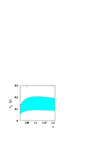
Figure 1: Universal form factor $\tau_{2}(y)$

We use the value $\hat{F}=0.21$ GeV^3/2, which is obtained by QCD sum rules [8, 15] with $\alpha_{s}=0$ (the same order which we consider in the present analysis). Moreover, we use $\Delta=0.5$ GeV, with the threshold in the $B$ channel $\omega_{c}=0.7$ GeV. As for the charm channel, we use $\omega_{1\,c}=\omega_{2\,c}=1.6-1.8$ GeV.

We can now numerically determine the form factors $\tau_{i}$, using the above equations. The result for the universal function $\tau_{1}(y)$, obtained within the uncertainties discussed above, is that this function, in the whole kinematical region relevant for the decays (20)-(21), is less than $10^{-4}$, which implies that, in the infinite heavy quark mass limit, the semileptonic $B$ transitions into the $s_{\ell}={3\over 2}^{-}$ doublet have a very small decay width. The situation is different for the universal function $\tau_{2}(y)$, which is depicted in fig.1 where the shaded region corresponds to the results obtained by varying the parameters $\Delta$, $\Delta_{2}$, $\omega_{c}$ and $\omega_{2c}$ in the ranges quoted above. The form factor $\tau_{2}$, at the zero recoil point $y=1$, is in the range $\tau_{2}(1)=0.10-0.20$, with a mild $y-$dependence that can be neglected, within the accuracy of the sum-rule method. Although it is difficult to reliably assess the theoretical accuracy of this result, it is interesting to observe that a form factor in the range quoted above implies that the semileptonic channel is experimentally accessible.

5 Semileptonic decay rates

Using the parameterization of the $B$ matrix elements in eqs.(26) and (27) we can work out the expressions of the widths of the decay modes (22) and (23), which are respectively given by:

$${d\Gamma\over dy}(B\rightarrow D^{*\prime}_{2}\ell\nu_{\ell})={G_{F}^{2}V_{cb}^{2}m_{B}^{2}m_{D^{*\prime}_{2}}^{3}\over 720\pi^{3}}(\tau_{2}(y))^{2}(y-1)^{5\over 2}(y+1)^{7\over 2}[(1+r^{2})(7y-3)-2r(4y^{2}-3y+3)]$$ (37)

$${d\Gamma\over dy}(B\rightarrow D_{3}\ell\nu_{\ell})={G_{F}^{2}V_{cb}^{2}m_{B}^{2}m_{D_{3}}^{3}\over 720\pi^{3}}(\tau_{2}(y))^{2}(y-1)^{5\over 2}(y+1)^{7\over 2}[(1+r^{2})(11+3y)-2r(11y+3)]$$ (38)

with $r={m_{D_{i}}\over m_{B}}$. Using $m_{D_{3}}=2.78$ GeV, $m_{D^{*\prime}_{2}}=2.74$ GeV and $\tau_{2}(y)=0.15$, we get

$$\Gamma(B\rightarrow D^{*\prime}_{2}\ell\nu_{\ell})\simeq\Gamma(B\rightarrow D_{3}\ell\nu_{\ell})\simeq 4\times 10^{-18}\;\;\;{\rm GeV}$$ (39)

and

$$B(B\rightarrow D^{*\prime}_{2}\ell\nu_{\ell})\simeq B(B\rightarrow D_{3}\ell\nu_{\ell})\simeq 1\times 10^{-5}\;\;\,\;.$$ (40)

Therefore, although small, semileptonic $B$ decays to the ${5\over 2}^{-}$ doublet are within the reach of the running $B$ factories, and could be experimentally observed, since the final mesons, as discussed in the next Section, are expected to be rather narrow.

As for $B$ decays to the ${3\over 2}^{-}$ doublet, due to the small value of the universal function $\tau_{1}$, the semileptonic widths turn out to be negligible at the leading order in the $1\over m_{Q}$ expansion (a discussion of the role of next-to-leading corrections for semileptonic $B$ decays to excited charm mesons can be found in [18]).

6 Remarks on strong decays of orbitally excited charm states

One might expect that the states in the multiplets $s_{\ell}^{P}={\frac{3}{2}}^{-}$ and ${\frac{5}{2}}^{-}$, being significantly higher in mass than the low-lying $s_{\ell}^{P}={\frac{1}{2}}^{-}$ multiplet, are rather broad. However this should be only true for the $s_{\ell}^{P}={\frac{3}{2}}^{-}$ states. As a matter of fact, the $J^{P}=2^{-}$ and $J^{P}=1^{-}$ states can decay into the $0^{-}$ or $1^{-}$ heavy meson plus one pion by $P-$wave transitions, which implies a kinematical suppression of the order of $\displaystyle\frac{|\vec{p}_{\pi}|^{3}}{\Lambda_{\chi}^{3}}$, where $\Lambda_{\chi}\simeq 1$ GeV is the typical chiral symmetry breaking scale. Taking into account that, for the charmed mesons, $|\vec{p}_{\pi}|\simeq 0.68$ GeV, we expect a kinematical phase space suppression, for this decay channel, of $\approx 0.3$.

On the other hand, for the mesons belonging to the multiplet $s_{\ell}^{P}={\frac{5}{2}}^{-}$, the decay into the low lying heavy meson and one pion occurs by $F-$wave transitions: the kinematical suppression is $\displaystyle\approx\frac{|\vec{p}_{\pi}|^{7}}{\Lambda_{\chi}^{7}}$, which numerically means a reducing factor $\approx 0.07$. Since the decay mode with one pion in the final state is expected to dominate the decay width, one may guess that the $3^{-}$ and $2^{-}$ mesons belonging to the $s_{\ell}^{P}={\frac{5}{2}}^{-}$ doublet are rather narrow .

To render these conclusions more quantitative, let us consider the effective lagrangian describing, in the chiral effective theory for heavy mesons [5], the strong couplings of the multiplet $H^{\mu\nu}$ to the pion and the multiplet $H$:

$${\mathcal{L}}=\frac{1}{\Lambda_{\chi}^{2}}Tr\left\{\bar{H}H^{\mu\nu}\left[k_{1}\{D_{\mu},D_{\nu}\}{\mathcal{A}}_{\lambda}+k_{2}\left(D_{\mu}D_{\lambda}{\mathcal{A}}_{\nu}+D_{\nu}D_{\lambda}{\mathcal{A}}_{\mu}\right)\right]\gamma^{\lambda}\gamma_{5}\right\}+h.c.$$ (41)

where $H$ is the $s_{\ell}^{P}={\frac{1}{2}}^{-}$ multiplet containing the $0^{-}$ and $1^{-}$ low-lying states, and $k_{1,2}$ effective couplings; moreover

$${\mathcal{A}}_{\lambda}={1\over 2}[\xi^{\dagger}\partial_{\lambda}\xi-\xi\partial_{\lambda}\xi^{\dagger}]$$ (42)

and $\xi=\exp[i{\vec{\pi}\cdot\vec{\tau}\over f_{\pi}}]$. Putting $\tilde{k}=k_{1}+k_{2}$, one obtains for the two-body decay widths:

$$\Gamma(D_{3}\to D\pi) = \frac{6\tilde{k}^{2}|\vec{p}_{\pi}|^{7}}{35\pi f_{\pi}^{2}\Lambda_{\chi}^{4}}\frac{m_{D}}{m_{D_{3}}}$$ (43)

$$\Gamma(D_{3}\to D^{*}\pi) = \frac{8\tilde{k}^{2}|\vec{p}_{\pi}|^{7}}{35\pi f_{\pi}^{2}\Lambda_{\chi}^{4}}\frac{m_{D^{*}}}{m_{D_{3}}}$$ (44)

$$\Gamma(D_{2}^{*\prime}\to D\pi) = 0$$ (45)

$$\Gamma(D_{2}^{*\prime}\to D^{*}\pi) = \frac{2\tilde{k}^{2}|\vec{p}_{\pi}|^{7}}{5\pi f_{\pi}^{2}\Lambda_{\chi}^{4}}\frac{m_{D^{*}}}{m_{D_{2}^{*\prime}}}$$ (46)

with $f_{\pi}\simeq 132$ MeV. The value of $\tilde{k}$ is unknown; however, on the basis of QCD sum rule results for similar couplings [9], one may assume $\tilde{k}\in[0.25,0.5]$. In correspondence to the lower bound in this range we get

$$\Gamma(D_{3}\to(D,D^{*})\pi) \simeq 32\;\;\;{\rm MeV}$$ (47)

$$\Gamma(D_{2}^{*\prime}\to D^{*}\pi) \simeq 15\;\;\;{\rm MeV}$$ (48)

where we have assumed the mass splitting of $40$ MeV between the $3^{-}$ and the $2^{-}$ mesons in the multiplet. There are other decay channels contributing to the full widths, but the corresponding partial widths are expected to be much smaller: for the decay modes with one pion and an excited positive parity $D$ resonance in the final state, occuring by $D-$wave transitions, we estimate a width of 1-2 MeV; for the decay modes with two pions and a heavy meson in the final state we expect, in the infinite heavy quark mass limit, a negligible contribution.

We can therefore conclude that reasonable estimates for the full widths of the $s_{\ell}={5\over 2}^{-}$ resonances are as follows:

$$\Gamma(D_{3}) = 35-140~{}{\rm MeV}$$ (49)

$$\Gamma(D^{*\prime}_{2}) = 17-70~{}{\rm MeV}\;\;\;\;,$$ (50)

a consideration which suggests the presence of a not too broad peak in the $D\pi$ and $D^{*}\pi$ channel in the region of $2.8$ GeV.

This conclusion, together with the result of a branching fraction of semileptonic $B$ decays to the ${5\over 2}^{-}$ doublet of the order of $10^{-5}$, encourages the experimental investigation at the currently running $B$-factories as well as at the hadronic facilities.

Acknowledgments

We thank Prof. R. Gatto and Prof. N. Paver for discussions and collaboration at an early stage of this work. (FDF) also acknowledges Département de Physique Théorique, Université de Genève, Switzerland, for hospitality, and “Fondazione Angelo Della Riccia” for financial support.

References

• [1] M.B. Voloshin and M.A. Shifman, Sov. J. Nucl. Phys. 45 (1987) 292; ibidem 47 (1988) 511; H.D. Politzer and M.B. Wise, Phys. Lett. B 206 (1988) 681; ibidem B 208 (1988) 504; N. Isgur and M.B. Wise, Phys. Lett. B 232 (1989) 113; ibidem B 237 (1990) 527; E. Eichten and B. Hill, Phys. Lett. B 234 (1990) 511; B. Grinstein, Nucl. Phys. B 339 (1990) 253; A.F. Falk, H. Georgi, B. Grinstein and M.B. Wise, Nucl. Phys. B 343 (1990) 1.
• [2] H. Georgi, Phys. Lett. B 240 (1990) 447.
• [3] C. Caso et al., Review of particle physics, Eur. Phys. J. C 3 (1999) 1.
• [4] CLEO Collaboration, S. Anderson et al., hep-ex/9908009.
• [5] A.F. Falk and M. Luke, Phys. Lett B 292 (1992) 119; U. Kilian, J.C. Körner and D. Pirjol, Phys. Lett. B 288 (1992) 360; R. Casalbuoni et al., Phys. Lett. B 299 (1993) 139; Phys. Rept. 281 (1997) 145.
• [6] V. Ciulli, hep-ex/9911044.
• [7] A.F. Falk, Phys. Lett. B 305 (1993) 268.
• [8] P. Colangelo, G. Nardulli, A.A. Ovchinnikov and N. Paver, Phys. Lett. B 269 (1991) 204; P. Colangelo, G. Nardulli and N. Paver, Phys. Lett. B 293 (1992) 207; P. Colangelo, F. De Fazio and N. Paver, Phys. Rev. D 58 (1998) 116005.
• [9] P. Colangelo et al., Phys. Lett. B 339 (1994) 151; P. Colangelo et al., Phys. Rev. D 52 (1995) 6422; P. Colangelo and F. De Fazio, Eur. Phys. J. C 4 (1998) 503.
• [10] Y.B. Dai et al., Phys. Lett. B 390 (1997) 350; Phys. Rev. D 55 (1997) 5719; Phys. Rev. D 58 (1998) 094032, ibid. D 59 (1999) 059901 (E); Phys. Rev. D 59 (1999) 034018.
• [11] S. Godfrey and R. Kokoski, Phys. Rev. D 43 (1991) 1679; A. Wambach, Nucl. Phys. B 434 (1995) 647; S. Veseli and M.G. Olsson, Phys. Lett. B 367 (1996) 302; Z. Phys. C 71 (1996) 287; Phys. Rev. D 54 (1996) 886; V. Morenas et al., Phys. Rev. D 56 (1997) 5668; A. Deandrea et al., Phys. Rev. D 58 (1998) 34004.
• [12] The BaBar Physics Book, P.F. Harrison and H.R. Quinn eds., SLAC-R-0504 (1998).
• [13] M. A. Shifman, A. I. Vainshtein and V. I. Zakharov, Nucl. Phys. B 147 (1979) 385; B 147 (1979) 448. For a review on the QCD sum rule method see: ”Vacuum structure and QCD Sum Rules”, edited by M. A. Shifman, North-Holland, 1992.
• [14] M. Neubert, Phys. Rev. D 45 (1992) 2451; D 47 (1993) 4063.
• [15] M. Neubert, Phys. Rept. 245 (1994) 259.
• [16] L.J. Reinders, H. Rubinstein and S. Yazaki, Phys. Rept. 127 (1985) 1.
• [17] A. Le Yaouanc, L. Oliver, O, Péne and J.C. Raynal, Phys. Rev. D 8 (1973) 2223; D 11 (1975) 1272; S. Godfrey and N. Isgur, Phys. Rev. D 32 (1985) 189; E.J. Eichten, C.T. Hill and C. Quigg, Phys. Rev. Lett. 71 (1993) 4116.
• [18] A.K. Leibovich, Z. Ligeti, I.W. Stewart and M.B. Wise, Phys. Rev. D 57 (1998) 308.
• [19] D. Melikhov and O. Péne, Phys. Lett. B 446 (1999) 336.