Cosmological Aspects of Heterotic M-theory

Abstract

In this talk we discuss a few relevant aspects of heterotic M-theory. These are the stabilization of the two relevant moduli (the length of the eleventh segment ($\pi\rho$) and the volume of the internal six manifold ($V$)) in models where supersymmetry is broken by multiple gaugino condensation and non-perturbative corrections to the Kähler potential; the existence of almost flat directions in the scalar potential; the possibility of lifting them, and their role in constructing a viable model of inflation. Finally, we review the status of the moduli problem within these models.

1 Introduction

As it was well established by Hořava and Witten [1], the strong coupling limit of the $E_{8}\times E_{8}$ heterotic string theory can be described by $d=11$ supergravity (SUGRA). This theory can be compactified on a manifold with boundaries, usually expressed as $X\times S^{1}/Z_{2}$, where $X$ is the $d=6$ Calabi–Yau manifold and $S^{1}/Z_{2}$ is the so-called eleventh segment. Altogether the picture we get is that of two walls (so-called hidden and observable) that interact through gravity.

The relevant parameters in this theory are $V$, the volume of the $d=6$ manifold, and $\pi\rho$, the length of the eleventh segment. Among the attractive features of this theory, it is worth mentioning the fact that gauge coupling unification is now entirely natural [2], and the scale at which the gauge couplings meet, $10^{16}$ GeV, is reconciled with the $d=4$ Planck scale, $M_{\rm P}\sim 10^{18}$ GeV. For this to happen, the process of compactification must occur in the order $d=11\rightarrow d=5\rightarrow d=4$. In other words, in ordet to fit the phenomenologically preferred values for $\alpha_{\rm GUT}$, $M_{\rm GUT}$ and $M_{\rm P}$, given by

$$\alpha_{\rm GUT} = (4\pi)^{2/3}\kappa^{4/3}\langle V\rangle^{-1}\;\;,$$

$$M_{\rm GUT} = \langle V\rangle^{-1/6}\;\;,$$ (1)

$$M_{\rm P} = \kappa^{-1}\sqrt{\pi\rho V}\;\;,$$

we need $\langle\pi\rho\rangle\sim(4\times 10^{15}\;{\rm GeV})^{-1}$ and $\langle V\rangle\sim(3\times 10^{16}\;{\rm GeV})^{-6}$. $\kappa^{2}$ is the $d=11$ gravitational coupling and its corresponding Planck scale is given by $M_{11}=\kappa^{-2/9}$.

Within this framework we are interested in studying phenomena such as supersymmetry (SUSY) breaking and the cosmological evolution of the moduli fields, which occur at scales below the compactification one. Therefore we shall concentrate on the $d=4$ effective SUGRA theory from now on.

2 Moduli stabilization

We shall discuss the stabilization of moduli as a previous step to address the question of their cosmological evolution. In order to do that, let us notice that the values of $V$ and $\pi\rho$ are determined by the chiral superfields $S$ (the dilaton) and $T$ (the modulus). More precisely the real parts of these chiral fields are given by

$$S_{\rm R} \sim \kappa^{4/3}V\sim O(\alpha_{\rm GUT}^{-1})\;\;,$$ (2)

$$T_{\rm R} \sim \kappa^{-2/3}\pi\rho V^{1/3}\sim O(\alpha_{\rm GUT}^{-1})\;\;.$$

Note that, in the weakly coupled heterotic case, $S_{\rm R}\sim O(\alpha_{\rm GUT}^{-1})\sim O(20)$, the same as here, whereas $T_{\rm R}\sim O(1)$ (always in $M_{\rm P}$ units).

To study the dynamical behaviour of these fields, and whether they acquire the desired vacuum expectacion values (VEVs), we analyse the scalar potential

$$V=e^{K}\left\{(W_{i}+K_{i}W)(K_{i}^{j})^{-1}(\bar{W}^{j}+K^{j}\bar{W})-3|W|^{2}\right\}\;\;,$$ (3)

where $W(S,T)$ is the superpotential and $K(S_{\rm R},T_{\rm R})$ is the Kähler potential. The sub (super) indices indicate derivatives of the functions with respect to the (conjugate) fields. Together with the gauge kinetic functions, $f_{a}$, $W$ and $K$ determine the SUGRA Lagrangian.

To be more precise, we shall assume a particular source for SUSY breaking, which is gaugino condensation in the hidden wall [3]. This is, so far, the most promising mechanism for breaking SUSY at the right scale in order to give rise to an acceptable phenomenology. It assumes the existence of a strong-type interaction in the hidden sector of the theory which, below a certain scale $\Lambda$, triggers the formation of gaugino condensates, $\lambda\lambda$, and the breakdown of SUSY. More precisely,

$$W\sim\langle\lambda\lambda\rangle\sim\sum_{i=1}^{N}C_{i}e^{-\alpha_{i}f_{i}}\;\;,$$ (4)

where the sum runs over all the condensing groups in the hidden sector ($G_{H}=G_{1}\times G_{2}\times\ldots\times G_{N}$), $\alpha_{i}$ are proportional to the 1-loop $\beta$-function coefficients associated to each condensing group, $C_{i}$ are also related to each group’s characteristics and $f_{i}$ are the already-mentioned gauge kinetic functions. In particular, in the hidden sector $f_{i}=(S-n_{i}T/2)/4\pi$, with $n_{i}$ being model dependent coefficients and, in the observable wall, $f_{\rm obs}=(S+n_{\rm obs}T/2)/4\pi$.

The Kähler potential is given by the expression

$$K=K_{0}+K_{\rm np}\;\;,$$ (5)

where $K_{0}=-\ln(2S_{\rm R})-3\ln(2T_{\rm R})$ is the tree level piece and $K_{\rm np}$ stands for M-theoretic non-perturbative effects. For the latter we will use a specific ansatz [4].

Now that we have defined all the functions we need to proceed with the analysis of the scalar potential, Eq. (3). We have first of all confirmed the results of Choi et al. [5] (obtained with a slightly different ansatz for $K_{\rm np}$), namely that for one condensate only the weakly coupled minimum exists. With two condensates ($W=C_{1}e^{-\alpha_{1}f_{1}}+C_{2}e^{-\alpha_{2}f_{2}}$), however, things become more interesting. It is possible to find plenty of examples of condensing groups for which both moduli are fixed at the desired VEVs and SUSY is broken at the right scale (i.e. the gravitino mass, $m_{3/2}$, is of order 1 TeV). In fact, in order to understand the vacuum structure a bit better, it is convenient to redefine the fields $S$ and $T$ as follows:

$\bullet$ The combinations

$$\Phi_{\rm r}^{-} \equiv S_{\rm R}-\frac{n_{1}\alpha_{1}-n_{2}\alpha_{2}}{2(\alpha_{1}-\alpha_{2})}T_{\rm R}\;,$$ (6)

$$\Phi_{\rm i}^{-} \equiv S_{\rm I}-\frac{n_{1}\alpha_{1}-n_{2}\alpha_{2}}{2(\alpha_{1}-\alpha_{2})}T_{\rm I}=\frac{4\pi^{2}k}{\alpha_{1}-\alpha_{2}}$$

are fixed by the interplay between condensates, very much in the same way as the racetrack mechanism worked in the weakly coupled heterotic case (note, from the second equation, that the condensates at the minimum, i. e. for $k$ odd, are in opposite phase).

$\bullet$ The orthogonal combinations are potentially flat

$$\Phi_{\rm r}^{+} \equiv \frac{n_{1}\alpha_{1}-n_{2}\alpha_{2}}{2(\alpha_{1}-\alpha_{2})}S_{\rm R}+T_{\rm R}\;,$$ (7)

$$\Phi_{\rm i}^{+} \equiv \frac{n_{1}\alpha_{1}-n_{2}\alpha_{2}}{2(\alpha_{1}-\alpha_{2})}S_{\rm I}+T_{\rm I}\;\;.$$

In fact we can easily check that these combinations of the fields do not appear in the superpotential. Therefore the potential flatness of $\Phi_{\rm r}^{+}$ will be lifted by the presence of the Kähler potential, which depends on $S_{\rm R}$, $T_{\rm R}$, whereas $\Phi_{\rm i}^{+}$ remains totally flat. This is a completely new feature associated to M-theory models, which depends entirely on the structure of the gauge kinetic functions $f_{a}$.

Let us proceed to analyse cases with more than two condensates. There the definitions of $\Phi_{\rm r,i}^{-}$ and $\Phi_{\rm r,i}^{+}$ can be easily generalized to many condensates, and it is also possible to show that the flat direction will only remain so if and only if all the $n_{i}$ coefficients that enter the definition of the gauge kinetic functions, $f_{i}$, are the same. This is shown in Fig. 1 where we plot the scalar potential as a function of $\Phi_{\rm i}^{\pm}$, for $\Phi_{\rm r}^{\pm}$ fixed, in the case of two (Fig. 1a) and three (Fig. 1b) condensates.

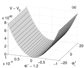
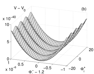
Figure 1: Scalar potential for (a) two condensates ${\rm SU}(3)_{M=0}\times{\rm SU}(4)_{M=8}$ with $n_{1}=n_{2}=1$, and (b) an additional third condensate ${\rm SU}(2)_{M=0}$ with $n_{3}=0.5$. $V_{0}$ is the value of the potential at the minimum.

As we can see, the flat direction of Fig. 1a is lifted by the presence of a third condensate with $n_{3}\neq n_{1}=n_{2}$. This opens up new scenarios from the cosmological point of view, as we are about to see.

3 Cosmological Evolution and Moduli Problem

Let us then study the possible cosmological role of the $\Phi^{\pm}_{\rm r,i}$ fields.

$\bullet$ $\Phi^{-}_{\rm r}$ has an exponential-type potential. In fact it is the analogous of the dilaton $S_{\rm R}$ in the weakly coupled heterotic string and will therefore suffer from the same problems [6]. The potential is too steep just before the minimum and the field tends to roll past it towards infinity. It can be, however, stabilized in the presence of a dominating background [7] but, in any case, it is totally unsuitable as an inflaton.

$\bullet$ $\Phi^{-}_{\rm i}$ has a steep sinusoidal potential, analogous to that of $S_{\rm I}$ in the weakly coupled heterotic case. Again, this field is not a good candidate for an inflaton.

On the other hand, the fields $\Phi_{\rm r,i}^{+}$ have more promising potentials, as it was pointed out above. It is then worth studying their evolution equations in the presence of an expanding Universe

$$K_{S\bar{S}}(\ddot{S}+3H\dot{S})+K_{SS\bar{S}}\dot{S}^{2}+\frac{\partial V}{\partial\bar{S}}=0\;\;,$$ (8)

$$K_{T\bar{T}}(\ddot{T}+3H\dot{T})+K_{TT\bar{T}}\dot{T}^{2}+\frac{\partial V}{\partial\bar{T}}=0\;\;,$$

where $H^{2}=\frac{1}{3}K_{S\bar{S}}\dot{S}\dot{\bar{S}}+\frac{1}{3}K_{T\bar{T}}\dot{T}\dot{\bar{T}}+\frac{V}{3}$ is the Hubble constant. It is crucial to note here that both $S$ and $T$ have non-minimal kinetic terms, i.e. ${\cal L}_{kin}=K_{S\bar{S}}D_{\mu}SD^{\mu}\bar{S}+K_{T\bar{T}}D_{\mu}TD^{\mu}\bar{T}$. This is what introduces the new terms in the evolution equations (8).

Let us start with the $\Phi_{\rm r}^{+}$ direction. It is easy to show that the potential along this direction behaves as an inverse power-law, i.e. $V(\Phi_{\rm r}^{+})=A/(\Phi_{\rm r}^{+})^{n}$, at least along the slope to the left of the minimum, which is the relevant one in terms of the evolution. By solving the evolution equations we have checked that the field inflates for a few e-folds before reaching its minimum. These kinds of inflationary scenarios are denoted as ‘intermediate’ inflation in the literature [8]. An important thing to notice is that, if the field $\Phi_{\rm r}^{+}$ were canonically normalized, then this inverse power-law potential would have given enough e-folds of inflation.

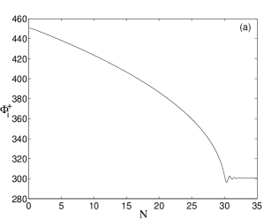
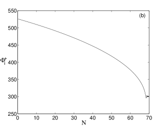
Figure 2: Evolution of $\Phi^{+}_{\rm i}$ as a function of $N$ (number of e-folds) for the three condensates of Figure 1b, with $n3=0.995$, and two different initial conditions. The real fields are fixed to their minimum values.

Finally we turn to the remaining direction to be analysed, namely $\Phi_{\rm i}^{+}$: as we had said before, in the two-condensate case this is a totally flat direction, however when we introduce a third condensate with $n_{3}\neq n_{1}=n_{2}$, things change. It can be shown that the potential in this latter case is a sinusoidal one,

$$V=V_{0}[1+\cos(a\Phi_{\rm i}^{+}+b)]\;\;,$$ (9)

where $a$ and $b$ are functions of $n_{3}$. It is easy to see that the closer $n_{3}$ is to $n_{1}$ and $n_{2}$ the flatter the potential is. Therefore we have a way of controlling the flatness of the potential, which can lead us to successful examples of inflation. A couple of them are shown in Fig. 2, where we plot $\Phi_{\rm i}^{+}$ as a function of the number of e-folds $N$. It is clear then that a combination of the imaginary parts of the dilaton $S$ and modulus $T$ fields, what we have denoted as $\Phi^{+}_{\rm i}$, can be a suitable inflaton in the context of heterotic M-theory. These are examples of the so-called natural inflation [9].

Let us finish this section by discussing very briefly the status of the moduli problem within these models. This arises when we have very weakly interacting particles with VEVs of the order of $M_{\rm P}$ and light masses, of the order of $m_{3/2}$. If these relics decay, they must do it before nucleosynthesis in order not to ruin its predictions. This imposes a lower bound on their masses of $\sim 10$ TeV. On the other hand, if these particles are stable, their oscillations should not overclose the Universe. This sets an upper bound of $\sim 10^{-24}$ eV on their masses. In the weakly coupled heterotic string case, where all moduli masses were of order $1$ TeV, these bounds were obviously difficult to fulfil [10].

We have calculated these masses for the present models. In general, we obtain that, along the $\Phi_{\rm r,i}^{-}$ directions, the corresponding masses are of the order of $10^{3}\;m_{3/2}$, well above the lower bound for decaying particles; along $\Phi_{\rm r}^{+}$ they are of the order of $10\;m_{3/2}$, which may be just enough to save the bound, and for $\Phi_{\rm i}^{+}$ they are very small and dependent on how close $n_{3}$ is to $n_{1}$, $n_{2}$. For example, for ${\rm SU}(3)_{M=0}\times{\rm SU}(4)_{M=8}\times{\rm SU}(2)_{M=0}$ with $n_{1}=n_{2}=1$ we find $m_{\Phi_{\rm i}^{+}}\sim 1.2\times 10^{-3}\;m_{3/2}$ for $n_{3}=0.98$ and $m_{\Phi_{\rm i}^{+}}\sim 1.5\times 10^{-4}\;m_{3/2}$ for $n_{3}=0.995$. There is therefore a conflict with the upper bound for stable particles, and the particle excess should be washed away with a period of thermal inflation [11].

4 Conclusions

We have studied the dynamics of the two typical M-theory moduli, namely $\pi\rho$ and $V$ in terms of $S$, $T$. In the presence of non-perturbative corrections to the Kähler potential, and gaugino condensation as the source of SUSY breaking, the scalar potential presents very interesting features.

$\bullet$ It depends on $S$, $T$ essentially through $f_{a}=S-n_{a}T/2$, motivating a redefinition of fields to $\Phi_{\rm r,i}^{-}$ and $\Phi_{\rm r,i}^{+}$.

$\bullet$ $\Phi_{\rm r,i}^{-}$ behave similarly to the dilaton of weakly coupled heterotic string theory: unsuitable as inflatons.

$\bullet$ $\Phi_{\rm r}^{+}$ would be flat in the absence of $K$: it has an inverse power-law potential, which gives very little intermediate inflation.

$\bullet$ $\Phi_{\rm i}^{+}$ is totally flat for two condensates and can have a sinusoidal potential for three or more: very promising inflaton (many e-folds of natural inflation).

$\bullet$ There might be a moduli problem associated to this almost flat direction. These lighter moduli can be diluted with a small period of weak scale inflation.

References

- [1] P. Hořava, E. Witten, Nucl. Phys. B 460, 506 (1996) and Nucl. Phys. B 475, 94 (1996).
- [2] E. Witten, Nucl. Phys. B 471, 135 (1996); T. Banks, M. Dine, Nucl. Phys. B 479, 173 (1996).
- [3] P. Hořava, Phys. Rev. D 54, 7561 (1996); Z. Lalak, S. Thomas, Nucl. Phys. B 515, 55 (1998); A. Lukas, B.A. Ovrut, D. Waldram, Phys. Rev. D 57, 7529 (1998) and JHEP 9904, 009 (1999).
- [4] T. Barreiro, B. de Carlos, E.J. Copeland, Phys. Rev. D 57, 7354 (1998).
- [5] K. Choi, H.B. Kim, H.D. Kim, Mod. Phys. Lett. A 14, 125 (1999).
- [6] R. Brustein, P.J. Steinhardt Phys. Lett. B 302, 93 (1993).
- [7] T. Barreiro, B. de Carlos, E.J. Copeland, Phys. Rev. D 58, 083513 (1998).
- [8] A.G. Muslimov, Class. Quant. Grav. 7, 231 (1990); J.D. Barrow, Phys. Lett. B 235, 40 (1990).
- [9] K. Freese, J.A. Frieman, A.V. Olinto, Phys. Rev. Lett. 65, 3233 (1990).
- [10] B. de Carlos, J.A. Casas, F. Quevedo, E. Roulet, Phys. Lett. B 318, 447 (1993); T. Banks, D.B. Kaplan, A.E. Nelson, Phys. Rev. D 49, 779 (1994).
- [11] D.H. Lyth, E.D. Stewart, Phys. Rev. Lett. 75, 201 (1995) and Phys. Rev. D 53, 1784 (1996); L. Randall and S. Thomas, Nucl. Phys. B 449, 229 (1995).