String formation and chiral symmetry breaking in the heavy–light quark–antiquark system in QCD

Abstract

The effective quark Lagrangian is written for a light quark in the field of a static antiquark, explicitly containing field correlators as coefficient functions of products of quark operators. At large $N_{c}$ the closed system of equations for the gauge–invariant quark Green’s function in the field of static source is examined analytically. The formation of the string connecting the light quark to the static source is observed numerically. The scalar Lorentz nature of the resulting confinement is shown to hold for the considered case, implying chiral symmetry breaking. The resulting spectrum with and without perturbative gluon exchanges is obtained numerically and compared to the $B$ and $D$ meson masses and HQET.

Pacs: 12.38Gc, 12.38Lg,12.39.Hg

I Introduction

The nature of QCD string formation between static sources was studied on the lattice [1, 2] and analytically [2]. From these investigations it was shown that the string consists of a predominantly color–electric longitudinal field. At the critical temperature $T_{c}$ this electric field disappears and and at the same time the deconfined phase with color–magnetic condensate sets in. This effect was predicted theoretically in [3] and also seen in lattice measurements[4]. At the same temperature Chiral Symmetry Breaking (CSB) for light quarks is found to disappear[5], which indicates that there is an intimate connection between the string formation and CSB. In the case of heavy quark systems CSB occurs due to the quark mass and confinement can be described as the area law of the Wilson loop. How CSB and confinement are explicitly realized for the light quark system and what equation describes its dynamics is an interesting and open problem.

It is the purpose of the present paper to study this issue in the simplest dynamical example – in the system of one light quark and a heavy antiquark. This allows us to describe the dynamics of light quark (its propagator) in a gauge–invariant manner, while physically the light quark is expected to be confined at the end of a string connected to the static source. Applying the formalism of field correlators (FC) [6, 7], we derive the effective quark Lagrangian, containing any number of quark operators multiplied by field correlators. To proceed further one can use the limit of large $N_{c}$ and write down the Dyson-Schwinger equations with the mass operator expressed through the Green’s function. The resulting equations are nonlocal and nonlinear. It is not clear from the beginning how confinement and CSB would manifest themselves in the solution of these equations. Some hint was provided in Ref. [8] using a relativistic WKB analysis [9], where it was shown that at large distances from the heavy source the dynamics of the light quark is described by the Dirac equation with a scalar linear confining interaction, which leads to CSB.

In this paper we examine the properties of the Green’s function of the color singlet $q\bar{Q}$ system, where the antiquark is treated in the static limit. In section II we formulate the full form of nonlocal and nonlinear equations for the light quark propagator and its eigenfunctions and study the behaviour at all distances. We also take into account both perturbative and nonperturbative contributions to the interaction kernel. As a result our equations contain both a confining interaction and color Coulomb part. Similar to the heavy quark situation we argue that the string formation for low angular momentum is of a color-electric nature. Moreover, the confinement of the light quark to the heavy one is shown to be of Lorentz scalar type. In section III the resulting nonlinear equations are studied numerically. The energy spectrum and the structure of the low lying eigenfunctions are presented. We in particular study the $B$ and $D$ meson spectrum. We compare them with experimental data for $B$, $D$ mesons and results of other calculations, exploiting for this purpose the expansion of Heavy Quark Effective Theory (HQET). In section IV the chiral condensate of the light quarks $\langle\bar{q}q\rangle$ is determined by taking the limit of the Green’s function $S(x,y)$, with both $x$ and $y$ tending to zero. In this limit the heavy quark is turned off and the condensate $\langle\bar{q}q\rangle\sim S(0,0)$ should have a value not depending on the presence of heavy quark.

II Derivation of equations

A Dyson-Schwinger equations

In this section we give an outline of the procedure to obtain the Dyson-Schwinger equations for the color white $q\bar{Q}$ system. Our starting point is the gauge–invariant light quark Green’s function $S(x,y)$ in the presence of a static heavy antiquark placed in the origin. In the static limit, the heavy quark can be treated as an external source. Assuming the Euclidean metric and letting $T=(x-y)_{4}$, the heavy antiquark propagator in the modified Fock-Schwinger gauge [10] is proportional to the parallel transporter,namely

$$S_{\bar{Q}}(A)=h({\bf x},{\bf y})\ Pexp(ig\int_{0}^{T}A_{4}({\bf r}=0,\tau)d\tau)$$ (1)

with

$$h({\bf x},{\bf y})=\frac{i}{2}\delta^{(3)}({\bf x}-{\bf y})[(1+\gamma_{4})\ e^{-m_{Q}T}\Theta(T)+(T\rightarrow-T,\gamma_{4}\rightarrow-\gamma_{4})].$$

This acts as a static source situated at the origin. As a result the proper limit for $m_{Q}\rightarrow\infty$ of the Green’s function of the $q\bar{Q}$ system can be defined as

$$S(x,y)=\langle\psi(x)\ \Pi(x,y)\ \psi^{+}(y)\rangle.$$ (2)

Here we have to average over the gluon fields $A$ and light quark fields $\psi$, while $\Pi$ contains the parallel transporters between the end points

$$\Pi(x,y)\equiv\phi({\bf x},x_{4};0,x_{4})\ \phi(0,x_{4};0,y_{4})\ \phi(0,y_{4};{\bf y},y_{4})$$

with

$$\phi({\bf x},x_{4};{\bf y},y_{4})=P~{}exp~{}ig\int^{y}_{x}A_{\mu}dz_{\mu}$$

.

The averaging over the gluon fields $A$ has to be done over the perturbative and nonperturbative gluon fields $a_{\mu}$ and $B_{\mu}$ contributions respectively, where the total gluonic field $A_{\mu}=B_{\mu}+a_{\mu}$. We now apply the method of field correlators (FC), which was developed in a series of papers [6, 7] to derive the effective quark Lagrangian from QCD. Let us first consider the effects of averaging over nonperturbative (NP) field $B_{\mu}$. We may write for the partition function

$$\langle Pe^{g\int\psi^{+}\hat{B}(x)\psi dx}\rangle_{B}\equiv e^{L_{eff}}=Pexp[\sum_{n}\frac{g^{n}}{n!}\int d^{4}x_{1}...d^{4}x_{n}j(1)...j(n)\langle\langle B(1)...B(n)\rangle\rangle]$$ (3)

with $j(n)\equiv j_{\mu_{n}}(x_{n})=\psi^{+}(x_{n})\gamma_{\mu_{n}}\psi(x_{n})$ and $B(n)=B_{\mu_{n}}(x_{n})$. To write the correlator $\langle\langle B...B\rangle\rangle$ for the gauge–invariant situation corresponding to the color white $q\bar{Q}$ system one can use the modified Fock-Schwinger gauge [10] to express the correlator of $B(x)$ through FC:

$$N(1,...n)\equiv\langle\langle B(1)...B(n)\rangle\rangle\sim\int dx(1)...dx(n)\langle\langle F(1)...F(n)\rangle\rangle.$$ (4)

The effective interaction kernel in Eq. (3) can now be used to write a Dyson–Schwinger–type equation for the quark Green’s function $S$. To simplify matter, one can consider the large $N_{c}$ limit, in which case the connected self–energy kernel $M(x,y)$ is obtained from Eq. (3) by replacing any pair of adjacent $\psi$–operators by

$$\psi_{a\alpha}(x)\psi^{+}_{a\beta}(y)\to N_{c}S_{\alpha\beta}(x,y),$$ (5)

where $a\alpha$ are color and Lorentz index respectively (for details of derivation see [8]). As a result one obtains the equation for $S(x,y)$

$$(-i\partial\!\!\!/_{x}~{}-im)S(x,y)-i\int M(x,z)S(z,y)d^{4}z=\delta^{(4)}(x-y),$$ (6)

where the kernel $M$ is expressed through $N$ as

$$iM(x,y) =N^{(2)}_{\mu\nu}(x,y)\gamma_{\mu}S(x,y)\gamma_{\nu}+$$ (8)

$$\sum^{\infty}_{n=3}\int d^{4}x_{2}...d^{4}x_{n-1}\gamma_{\mu_{1}}S(x,x_{2})\gamma_{\mu_{2}}...\gamma_{\mu_{n-1}}S(x_{n-1},y)\gamma_{\mu_{n}}N^{(n)}_{\mu_{1}...\mu_{n}}(x,x_{2}...x_{n-1},y).$$

The system of equations (6-7) is exact in the large $N_{c}$ limit and is well defined provided all NP correlators $\langle\langle F(1)...F(n)\rangle\rangle$ are known.

Evidence has been found in recent accurate lattice calculations [11] of static potentials in different $SU(3)$ representations, that the contributions of the higher correlators $\langle\langle F(1)...F(n)\rangle\rangle$ for $n>2$ to the planar Wilson loop are small. In particular, these terms are found to contribute only around a few percent of the dominant Gaussian correlator [12]. Hence, the Gaussian Stochastic Model, based on the lowest correlator $\langle\langle F(1)F(2)\rangle\rangle$ is expected to be a good approximation. In view of this we assume in this paper that the Gaussian approximation holds and we keep similar as in Ref. [8] only the first term in Eq. (8). One can parametrize the Gaussian correlator according to [6] as

$$\langle\langle F(1)F(2)\rangle\rangle=\frac{1}{N_{c}}tr\langle F_{\mu\lambda}(x)\phi(x,0)F_{\nu\sigma}(0)\phi{(0,x)}\rangle=D(x)(\delta_{\mu\nu}\delta_{\lambda\sigma}-\delta_{\mu\sigma}\delta_{\nu\lambda})+\Delta^{(1)}_{\mu\lambda\nu\sigma},$$ (9)

where only $D(x)$ is responsible for confinement and it contributes to string tension $\sigma$, while $\Delta^{(1)}$ is a full derivative. As a consequence, the latter contributes to the perimeter of Wilson loop and $\phi(x,0)=P~{}exp~{}ig\int^{x}_{0}B_{\mu}dz_{\mu}$. From this we find, that the $N^{(2)}_{\mu\nu}$ can explicitly be written in the gauge [10] as

$$N_{\mu\nu}^{(2)}(x,y)=(\delta_{\mu\nu}\delta_{ik}-\delta_{\mu k}\delta_{\nu i})\int^{x}_{0}du_{i}\alpha_{\mu}(u)\int^{y}_{0}dv_{k}\alpha_{\nu}(v)D(u-v),$$ (10)

where $\alpha_{4}(u)=1,\alpha_{i}(u)=\frac{u_{i}}{x_{i}}$.

In Eq. (10) only the nonperturbative confining piece of the Gaussian correlator (9) is retained, since the perturbative part and $\Delta^{(1)}$ do not produce neither the string (confinement) nor CSB [8]. In the case of a nonrotating string the terms in Eq. (7) with space components $\gamma_{k}$ are suppressed by powers of velocity of the endpoints of the string. In what follows we shall keep for simplicity only the component $N_{44}^{(2)}\equiv J(x,y)$ of $N_{\mu\nu}^{(2)}$. Hence the kernel $M$ is proportional to the FC of the color–electric field $E_{i}\equiv F_{i4}$. It is the dominant part of the string. Color–magnetic components are neglected in this first step and can be considered as a correction.

In this way one arrives at the system of equations [8] where we keep the same notation $M(x,y)$ for the retained piece of the kernel

$$iM(x,y)=J(x,y)\gamma_{4}S(x,y)\gamma_{4}$$ (11)

$$(-i\partial\!\!\!/_{x}~{}-im)S(x,y)-i\int M(x,z)S(z,y)d^{4}z=\delta^{(4)}(x-y).$$ (12)

B Partial wave reduced equations

The kernel $J(x,y)$ in Eq. (11) depends on the time as $\frac{x_{4}-y_{4}}{T_{g}}$. Therefore in the limit of $T_{g}\to 0$ it becomes local in time. As a result, the Fourier–transform of $M$ in the fourth coordinate does not depend on the momentum $p_{4}$ for $T_{g}\to 0$. The corresponding eigenfunctions $\psi_{n}(\mbox{\boldmath${\rm x}$},p_{4})=\psi_{n}(\mbox{\boldmath${\rm x}$})$ and eigenvalues $\varepsilon_{n}=\varepsilon_{n}(p_{4})$ of the light quark in the white light-heavy configuration can readily be obtained from Eqs. (11-12) in the discussed instantaneous limit. We find

$$(\frac{\mbox{\boldmath${\rm\alpha}$}}{i}\frac{\partial}{\partial\mbox{\boldmath${\rm x}$}}+\beta m)\psi_{n}(\vec{x})+\beta\int M(\mbox{\boldmath${\rm x}$},\mbox{\boldmath${\rm z}$})\psi_{n}(\mbox{\boldmath${\rm z}$})d^{3}\mbox{\boldmath${\rm z}$}=\varepsilon_{n}\psi_{n}(\mbox{\boldmath${\rm x}$})$$ (13)

$$M(\mbox{\boldmath${\rm x}$},\mbox{\boldmath${\rm z}$})=J(\mbox{\boldmath${\rm x}$},\mbox{\boldmath${\rm z}$})\beta\Lambda(\mbox{\boldmath${\rm x}$},\mbox{\boldmath${\rm z}$}),\ \ \ \Lambda(\mbox{\boldmath${\rm x}$},\mbox{\boldmath${\rm z}$})=\sum_{k}\psi_{k}(x)sign\varepsilon_{k}\psi^{+}_{k}(z)$$ (14)

The spherical–spinor decomposition of $\psi_{n}$ for the total and orbital angular momentum channel $j$, $l=j\pm\frac{1}{2}$,

$$\psi_{n}(r)=\frac{1}{r}\left(\begin{array}[]{l}G_{n}(r)\Omega_{jlM}\\ iF_{n}(r)\Omega_{jl^{\prime}M}\end{array}\right),l^{\prime}=2j-l$$ (15)

yields equations for the partial waves

$$\frac{dF_{n}}{dr}-\frac{\kappa}{r}F_{n}+(\varepsilon_{n}-m)G_{n}-M_{11}G_{n}-iM_{12}F_{n}=0$$ (16)

$$\frac{dG_{n}}{dr}+\frac{\kappa}{r}G_{n}-(\varepsilon_{n}+m)F_{n}-M_{22}F_{n}+iM_{21}G_{n}=0$$ (17)

with $\kappa=\pm(j+\frac{1}{2})$. Clearly the kernels $M_{ik}$ are nonlocal in space, i.e.

$$M_{ik}G_{n}=\int^{\infty}_{0}M^{jj}_{ik}(r,r^{\prime})~{}G_{n}(r^{\prime})rr^{\prime}dr^{\prime}$$ (18)

with $M^{jj}_{ik}=\langle\Omega_{jl_{i}M}|M_{ik}|\Omega_{jl_{k}M}\rangle$ and $M_{ik}$ is given by Eq. (14).

Equations (16-17) are invariant under the transformation

$$\varepsilon_{n}\to-\varepsilon_{n},\ \ \kappa\leftrightarrow-\kappa,\ \ G_{n}\leftrightarrow F_{n}$$ (19)

which also yields $M_{11}\leftrightarrow M_{22},M_{12}\leftrightarrow-M_{21}.$ The symmetry (19) implies that the spectrum is symmetric in $\varepsilon_{n}\leftrightarrow-\varepsilon_{n}$, which is a property of a scalar interaction. The Lorentz scalar nature of the confining interaction has the nice feature that it doesnot lead to instability problems in the Dirac equation [14]. Moreover, nontrivial solutions of Eqs. (16-17), if they exist, signify spontaneous CSB.

We solve Eqs. (16-17), using the relativistic WKB approximation for the kernel $M_{ik}$. To simplify the calculations the Gaussian form for $D(x)$ was used (since all observables are integrals of FC, its explicit form is not essential at large distances, provided the FC have a finite range $T_{g}$ and it yields the same value of the string tension $\sigma$)

$$D(u)=D(0)exp(-u^{2}/4T^{2}_{g}),\ \ D(0)=\frac{\sigma}{2\pi T^{2}_{g}}$$ (20)

with $\sigma=0.2~{}GeV^{2},$ and $T_{g}=0.25~{}fm$, taken in accordance with the lattice measurements [4, 13].

As the reference basis we take the WKB solutions of the Dirac equation for the local linear confining potential $\sigma r$, and the WKB computed kernels $\tilde{M}$ and $\tilde{\Lambda}(\mbox{\boldmath${\rm x}$},\mbox{\boldmath${\rm y}$})$ in Eq. (14) are determined by explicit summation over eigenstates. It was checked by an independent calculation [15] that the relativistic WKB procedure yields eigenvalues of the linear potential with accuracy better than one percent.

The general structure of $M$ and $\tilde{M}$ can be derived from Eqs. (14-15). One can write $M$ as a $4\times 4$ matrix as follows [16]

$$M=M^{(0)}I+M^{(i)}\hat{\sigma}_{i}+M^{(4)}\gamma_{4}+M_{\gamma}^{(i)}\gamma_{i},$$ (21)

where $\gamma_{i},\gamma_{4}$ are usual Dirac matrices, $i=1,2,3$ and $\hat{\sigma}_{i}=\left(\begin{array}[]{ll}\sigma_{i}&0\\ 0&\sigma_{i}\end{array}\right)$.

The same representation holds for the WKB approximated $\tilde{M}$. From the WKB analysis [8, 16] we find that $\tilde{M}^{(0)}$ is the only growing kernel. It behaves asymptotically as

$$M^{(0)}(\mbox{\boldmath${\rm x}$},\mbox{\boldmath${\rm y}$})=\sigma\frac{|\mbox{\boldmath${\rm x}$}+\mbox{\boldmath${\rm y}$}|}{2}\tilde{\delta}^{(3)}(\mbox{\boldmath${\rm x}$}-\mbox{\boldmath${\rm y}$})$$ (22)

where $\tilde{\delta}^{(3)}(\mbox{\boldmath${\rm r}$})$ is a smeared $\delta$ – function with the range of nonlocality decreasing asymptotically with growing $|\mbox{\boldmath${\rm x}$}|$, $|\mbox{\boldmath${\rm y}$}|$. The term $M^{(i)}$ is proportional to the angular momentum $L$ and asymptotically it behaves as $O(1/x)$. One can also prove that $M^{(4)},M_{\gamma}^{(i)}$ do not grow at large $x,y$ [16]. Hence in all problems where large distances are dominant one can consider only the first term in Eq. (21). Using this approximation we get for the kernel (14)

$$\tilde{M}=\tilde{M}^{(0)}(\mbox{\boldmath${\rm x}$},\mbox{\boldmath${\rm y}$})I=J(\mbox{\boldmath${\rm x}$},\mbox{\boldmath${\rm y}$})\tilde{\Lambda}(\mbox{\boldmath${\rm x}$},\mbox{\boldmath${\rm y}$})I$$ (23)

with

$$J({\bf x},{\bf y})=\sigma\frac{{\bf x}{\bf y}}{\sqrt{\pi}}f({\bf x},{\bf y}),\ \ f({\bf x},{\bf y})=\int^{1}_{0}ds\int^{1}_{0}dte^{-\frac{({\bf x}s-{\bf y}t)^{2}}{4T^{2}_{g}}}$$ (24)

and where $\tilde{\Lambda}$ is now a scalar quantity.

A curious feature of the considered equations is the way how the string connecting the light quark to the source is being created. Actually, if one takes only lowest partial waves inside the kernel $M$ (i.e. in $\Lambda(\mbox{\boldmath${\rm x}$},\mbox{\boldmath${\rm y}$})$, Eq. (14)), then the effective potential in Eqs. (16-17) is not confining. If one however sums up over all angular states and radial excitations in $\Lambda$, then the resulting $\Lambda(x,y)$ is a smeared $\delta$– function leading to the quasilocal confining kernel $\tilde{M}$. E.g. using eigenfunctions for the local case, $\tilde{\Lambda}$ can be computed quasiclassically to be

$$\tilde{\Lambda}(\mbox{\boldmath${\rm x}$},\mbox{\boldmath${\rm y}$})=\frac{\sigma^{2}xy}{2\pi^{2}}\frac{K_{1}(\sigma\sqrt{xy}\sqrt{(x-y)^{2}+\theta^{2}xy)}}{\sqrt{(x-y)^{2}+\theta^{2}xy}},\ \ \mbox{\boldmath${\rm x}$}\mbox{\boldmath${\rm y}$}=xy\cos\theta$$ (25)

In Eq. (25) one can clearly see that $\tilde{\Lambda}(x,y)$ is a normalized smeared $\delta$–function, with smearing radius in $|x-y|$ being $\frac{1}{\sigma\sqrt{xy}}$. For large distances it is nonvanishing only in the forward direction.

Insertion of this $\tilde{\Lambda}$ into $\tilde{M}$, Eq. (23), produces linear confinement due to the kernel $\tilde{\Lambda}(\mbox{\boldmath${\rm x}$},\mbox{\boldmath${\rm y}$})$, as is given by Eq. (25) (while simply averaging the contribution from each individual orbital in Eq. (14) over the angle between ${\rm x}$ and ${\rm y}$ would produce no confinement at all). The computed kernel $\tilde{M}(x,y)$ turns out to be nonlocal, but very close to the linear potential at large distances. Indeed, the effective localized potential defined as

$$V_{eff}(r)={\int M^{(0)}(r,x)rx{dx}}$$ (26)

approaches at very large distances, i.e. for $\sigma^{1/2}r>200$, a linear dependence with a slope given by $\sigma$. However at shorter distances $V_{eff}$ looks also linear over a relatively large region with a slope almost the same as $\sigma$, reflecting the presence of a small local curvature. In particular, we find that in the region $5<\sigma^{1/2}r<20$ the effective potential can reasonable well be described by $V_{0}(r)=0.9\sigma r-1.8\sigma^{1/2}$. In Fig. 1 are shown the results up to $r=20$ in units of $\sigma^{1/2}$.

Since it is only the higher states and large distances which are important in the creation of this $\delta$ – function–type behaviour of $\Lambda(x,y)$, and since the WKB method does well for high states and at large distances, one can clearly conclude, that linear confinement should be obtained if one sums over all exact solutions of Eqs. (16-17). Hence this should be a property of the exact solution.

The property, that the kernel has a focussing effect in the forward direction can be used to get a somewhat simpler form. For this purpose we may also use [8]

$$\tilde{\Lambda}(\mbox{\boldmath${\rm x}$},\mbox{\boldmath${\rm y}$})=\frac{\sigma}{\pi^{2}\sqrt{xy}}K_{0}(a)\delta(cos\theta_{x}-cos\theta_{y}),\ \ a=\sigma\sqrt{xy}|x-y|$$ (27)

The eigenvalues and eigenfunctions in Eqs. (16-17) have been determined using the kernel $\tilde{M}(x,y)$, given by Eqs. (25) and (27). Some results are shown in Table 1 and Fig. 2. In our present study we have taken $m=0$. Note, that $\tilde{M}(x,y)$ is approaching a local linear potential at large distances, $x,y\mathrel{\mathchoice{\lower 3.6pt\vbox{\halign{$\mathsurround=0pt\displaystyle\hfil#\hfil$\cr>\crcr\sim\crcr}}}{\lower 3.6pt\vbox{\halign{$\mathsurround=0pt\textstyle\hfil#\hfil$\cr>\crcr\sim\crcr}}}{\lower 3.6pt\vbox{\halign{$\mathsurround=0pt\scriptstyle\hfil#\hfil$\cr>\crcr\sim\crcr}}}{\lower 3.6pt\vbox{\halign{$\mathsurround=0pt\scriptscriptstyle\hfil#\hfil$\cr>\crcr\sim\crcr}}}}\sigma^{-1/2}$, which justifies a posteriori our choice of the reference basis. Due to the nonlocality of the interaction the predicted spectrum is found to be different from that of the linear potential, valid at large distances. Moreover, comparing the level structures of the $J=\frac{1}{2}$ channel as obtained using the kernels (25) and (27) we see from Table I, that they are qualitatively very similar, corroborating that there is indeed a strong forward focussing effect in the quark propagator. From Fig. 2 we see that for all L values the higher radially excited levels are close to the predictions of linear potential $V_{0}(r)=0.9\sigma r-1.8\sigma^{1/2}$, in agreement with the fact that the interaction at large distance can indeed be described by a local linear potential. On the other hand the nonlocal kernel predictions for the low lying states clearly deviates strongly from those of the (shifted) linear potential. Hence the nonlocal nature of the force does affect the spectrum in an essential way.

The eigenfunctions for the nonlocal kernels look qualitatitively similar to the corresponding ones of the shifted linear potential. In Fig. 3 are shown the ground state and first excited state for the $J=\frac{1}{2}$ channels. Altough the differences are substantial for these low lying states, the agreement for higher excited states is considerably better. Moreover, we find that the large distances and high states of the WKB states agree well with the corresponding eigenfunctions.

C Inclusion of perturbative exchanges

Till now we have considered only NP part of the gluonic field, $B_{\mu}$. In this section we include the perturbative part, $a_{\mu}$, and neglect for simplicity the interference terms. Therefore the effect of $a_{\mu}$ is accounted for in the appearance of an additional factor in the partition function (3), namely

$$Z=Z_{NP}Z_{pert},\ \ Z_{pert}=\langle e^{g\int dx\psi^{+}\hat{a}(x)\psi(x)+ig\int dz_{4}a_{4}(z_{4})}\rangle_{a},$$ (28)

where the second term in the exponent of (28) corresponds to the interaction of the perturbative part of the gluon field with the static antiquark. We have used in (28), that due to the ’tHooft identity [17] one can average independently over $B_{\mu}$ and $a_{\mu}$.

The result of averaging yields a new additive term in $L_{eff}$, Eq. (3),

$$L_{c}=g\int dx\psi^{+}(x)\hat{A}^{(c)}(x)\psi(x),$$ (29)

where we have defined

$$A_{\mu}^{(c)}(x)=-ig\int dz_{4}<a_{4}(x)a_{4}(z_{4})>=\delta_{\mu 4}\frac{(-i)gC_{2}}{4\pi|\mbox{\boldmath${\rm x}$}|}.$$ (30)

The presence of $L_{c}$ in Eq. (3) does not influence the derivation of basic Eqs. (11-12). The only difference is that Eq. (12) assumes the form

$$(-i\hat{\partial}-g\hat{A}^{c}(x)-im)S(x,y)-i\int M(x,z)S(z,y)d^{4}z=\delta^{(4)}(x-y).$$ (31)

Eq. (11) does not change and the kernel $J(x,y)$ contains as before only nonperturbative contributions. Note however that $S(x,y)$ in $M(x,y)$ in Eq. (11) now contains also perturbative gluon exchanges. This is a new type of interference of perturbative and NP terms, which appears irrespectively of our neglect of this interference within the averaging procedure over $B_{\mu}$ and $a_{\mu}$. In other words another class of diagrams is responsible for this interference.

Correspondingly in the static equations (13) one should replace

$$\beta m\to\beta m-\frac{C_{2}\alpha_{s}}{|\mbox{\boldmath${\rm z}$}|}$$ (32)

The equations for the partial waves (16-17) are modified due to the presence of the color Coulomb potential $V(r)$ in a simple way. Since

$$V(r)=-\frac{C_{2}\alpha_{s}}{r}$$ (33)

is local and a Lorentz vector, it always appears in the combination $\varepsilon_{n}-V(r)$. Hence one has instead of Eqs. (16-17)

$$\frac{dF_{\nu}}{dr}-\frac{\kappa}{r}F_{\nu}+(\varepsilon_{\nu}-V(r)-m)G_{\nu}-M_{11}G-iM_{12}F=0,$$ (34)

$$\frac{dG_{\nu}}{dr}+\frac{\kappa}{r}G_{\nu}-(\varepsilon_{\nu}-V(r)+m)F_{\nu}-M_{22}F+iM_{21}G=0,$$ (35)

where we have denoted

$$M_{ik}\left(\begin{array}[]{l}G\\ F\end{array}\right)\equiv\int<\nu|M_{ik}|\nu^{\prime}>\left(\begin{array}[]{l}G_{\nu^{\prime}}(w)\\ F_{\nu^{\prime}}(w)\end{array}\right)rwdw.$$ (36)

Here $M_{ik}$ is defined as in Eq. (14) and the matrix $\Lambda_{ik}$ in Eq. (14) involves the sum over all states, including positive and negative $\varepsilon_{n}$. There in section IIB we have exploited the symmetry (19). However Eqs. (34-35) are invariant under another transformation, namely

$$\varepsilon_{n}\leftrightarrow-\varepsilon_{n},V(r)\leftrightarrow-V(r),\kappa\leftrightarrow\kappa,G_{n}\leftrightarrow F_{n}.$$ (37)

Now the sum over negative $\varepsilon_{n}$ can be expressed through the corresponding sum over positive $\varepsilon_{n}$ with exchange $G_{n}\leftrightarrow F_{n}$ as before, but also with the inversion of sign of Coulomb interaction, i.e. Coulomb attraction for positive $\varepsilon_{n}$ is replaced by Coulomb repulsion for negative $\varepsilon_{n}$.

In what follows we shall denote wave functions of the positive energy states with repulsive Coulomb with the sign of tilde: $\tilde{G}_{\nu},\tilde{F}_{\nu}$. Then using (14) the matrix $\beta\Lambda_{ik}$ can be written as a sum over only positive $\varepsilon_{n}$ as follows

$$\beta\Lambda^{\mu\mu^{\prime}}_{ik}=\frac{1}{xy}\sum_{jlM,n>0}\left(\begin{array}[]{ll}~{}~{}~{}~{}G_{\mu}G_{\mu^{\prime}}^{*}-\tilde{F}_{\mu}\tilde{F}^{*}_{\mu^{\prime}},&-i(G_{\mu}F^{*}_{\mu^{\prime}}-\tilde{F}_{\mu}\tilde{G}^{*}_{\mu^{\prime}})\\ -i(F_{\mu}G_{\mu^{\prime}}^{*}-\tilde{G}_{\mu}\tilde{F}^{*}_{\mu^{\prime}}),&~{}~{}~{}~{}\tilde{G}_{\mu}\tilde{G}^{*}_{\mu^{\prime}}-F_{\mu}F^{*}_{\mu^{\prime}}\end{array}\right).$$ (38)

Since $\beta\Lambda$ is exactly the combination which enters the mass matrix (14), one can list in (38) scalar and vector (proportional to $\beta)$ parts:

$$M=M_{s}I+M_{v}\beta+\Delta M,$$ (39)

where $\Delta M$ contains spin-dependent terms, which can be considered as in section IIB, while $M_{s}$, $M_{v}$ are

$$M_{s,v}=C\sum_{jlM\mu,n>0}[G_{\mu}G^{*}_{\mu}-\tilde{F}_{\mu}\tilde{F}^{*}_{\mu}\pm(\tilde{G}_{\mu}\tilde{G}_{\mu}-F_{\mu}F^{*}_{\mu})]$$ (40)

where

$$C=\frac{1}{4}\sqrt{\pi}T_{g}D(0)\frac{\mbox{\boldmath${\rm x}$}\cdot\mbox{\boldmath${\rm y}$}}{xy}f(\mbox{\boldmath${\rm x}$},\mbox{\boldmath${\rm y}$}),~{}~{}f({\bf x},{\bf y})=\int^{1}_{0}ds\int^{1}_{0}dt~{}exp\left(-\frac{({\bf x}s-{\bf y}t)^{2}}{4T^{2}_{g}}\right).$$ (41)

From (40) it is clear that the vector part $M_{v}$ is only due to the presence of Coulomb interaction. Corrections at large distances due to the vector part can be treated again in the relativistic WKB. A rough estimate of $M_{v}$ at large $r$ yields

$$\frac{M_{v}}{M_{s}}\sim\frac{\alpha_{s}}{\sigma r^{2}}$$ (42)

and hence can be neglected at large enough $r$.

III Numerical solutions of equations and comparison to $B$, $D$ mesons

We have performed numerical studies of Eqs. (34-35) with the kernel (25) for different values of the quark mass $m$ and different values of $T_{g}$. To simplify calculations only the dominant part of the mass operator $M_{ik}$ was retained, i.e. $\hat{M}_{11}=M_{22}=M^{(0)}$, while $M_{12},M_{21}$ have been neglected. For $M^{(0)}$ the representation (23) was used

$$M^{(0)}({\bf x},{\bf y})=J({\bf x,}{\bf y})\tilde{\Lambda}({\bf x},{\bf y})I,$$

where $\tilde{\Lambda}$ is taken to be the kernel (25). Results of our calculations for the ground state energy are listed in Table 2. One can see a rather sharp change of energy when $\alpha_{s}$ changes from 0 to 0.3 and when $T_{g}$ is changing from 0 to 0.25, while further increase of $\alpha_{s}$ or $T_{g}$ does not produce such a strong dependence.

Solutions of our equations (34-35) can be compared with physical states of $B$, $D$ and $B_{s},D_{s}$ mesons. To this end one should have in mind that in Eqs. (34-35) the static approximation for the heavy quark $b,c$ was used, and hence all corrections $O(1/m^{n}_{Q})$ with $n\geq 1$ are neglected.

One can exploit at this point the HQET expansion for the mass $m_{H}$ of heavy–light boson [18, 19]

$$m_{H}=m_{Q}(1+\frac{\bar{\Lambda}}{m_{Q}}+\frac{1}{2m^{2}_{Q}}(\lambda_{1}+d_{H}\lambda_{2})+O(1/m^{3}_{Q}),$$ (43)

where $\lambda_{n}$ are free parameters, depending on dynamics, and $d_{H}$ is the hyperfine splitting parameter. It is clear from the preceding that eigenvalues of Eqs. (34-35) yield the value $\bar{\Lambda}$, which depends on the quantum numbers of the state,

$$\bar{\Lambda}(j,l,n_{r})=\varepsilon_{n}(j,l)$$ (44)

Consider now the results of the present approach, i.e. solutions of Dirac–type equations (34-35). In the local case $(T_{g}\to 0)$ when the kernel $M$ reduces to the linear potential $\sigma r$, we have

$$\bar{\Lambda}_{D}^{(loc)}=0.690~{}GeV~{}~{}(\alpha_{s}=0,~{}~{}\sigma=0.18~{}GeV^{2})$$ (45)

and

$$\bar{\Lambda}_{D}^{(loc)}=0.493~{}GeV~{}~{}(\alpha_{s}=0.3,~{}~{}\sigma=0.18~{}GeV^{2}).$$ (46)

This should be compared to the nonlocal case

$$\bar{\Lambda}_{D}^{(nonloc)}=0.415~{}GeV~{}~{}(\alpha_{s}=0,~{}~{}\sigma=0.18~{}GeV^{2})$$ (47)

and

$$\bar{\Lambda}_{D}^{(nonloc)}=0.288~{}GeV~{}~{}(\alpha_{s}=0.3,~{}~{}\sigma=0.18~{}GeV^{2}).$$ (48)

These latter values are in general agreement with the results of the QCD heavy–flavour sum rules [20, 21]

$$\bar{\Lambda}=0.57\pm 0.07~{}GeV$$ (49)

and more recent analysis from semileptonic $B$ decays [22]

$$\bar{\Lambda}=0.39\pm 0.11~{}GeV$$ (50)

Another interesting comparison is with the experimental values of the $B$–meson mass (the term $\lambda_{2}$ in Eq. (43) can be determined from the $B^{*}-B$ mass difference). Using Eq. (48) and $\bar{M}_{B}=\frac{3M_{B^{*}}+M_{B}}{4}=5.312~{}GeV$ one can estimate (neglecting $\lambda_{1})$ the pole mass of the $b$–quark to be $m_{b}(pole)\cong 5.0~{}GeV$, which is in reasonable agreement with the analysis of the quarkonium spectra in [23].

A similar analysis can be done for the $B_{s}$ meson; the corresponding values for $\bar{\Lambda}_{s}$ with $m_{s}=0.15$ and 0.20 $GeV$, are $\bar{\Lambda}_{s}-\bar{\Lambda}=0.084$ and $\bar{\Lambda}_{s}-\bar{\Lambda}=0.115$ for $\alpha_{s}=0.3$ . One can compare these values with the mass difference $B_{s},B^{0},\Delta M_{s}(B)=(0.090\pm 0.0038)~{}GeV$. These numbers for $\bar{\Lambda}$ can be compared with those in Table 3, where also results of lattice calculations [24] and of the constituent quark model (CQM) [25, 26, 27] are given.

IV Chiral condensate

As a check of CSB in our Eqs. (16-17) we have computed the chiral condensate, which can be expressed through the eigenfunctions as in [8] (to simplify matter we disregard in this section perturbative contributions).

$$\langle\bar{q}q\rangle=-\frac{N_{c}}{2\pi}\sum^{\infty}_{n=0}[(A^{-}_{n})^{2}-(B^{+}_{n})^{2}],$$ (51)

where $A^{-}_{n}=(\frac{G_{n}(r)}{r})_{r=0},B^{+}_{n}=(\frac{F_{n}(r)}{r})_{r=0}$, and $G_{n},F_{n}$ refer to solutions with $\kappa=-1,l=0$ and $\kappa=+1,l=1$ respectively. In the local linear potential case the values of $A^{-}_{n},B^{+}_{n}$ have been computed in the WKB method [8] and shown to yield a monotonically divergent series $\langle\bar{q}q\rangle=-\frac{N_{c}}{2\pi}\sum_{n}\frac{const}{\sqrt{n}}$.

It can be argued (using Eqs. (8-9) from [8]), that the nonlocality of the kernel $M$ in space–time, present by definition in Eq. (8) improves the convergence of the series and yields a finite result for $\langle\bar{q}q\rangle$. We have found $A_{n}^{-},B_{n}^{+}$ from the solutions of the nonlocal equations (16-17) with the kernel $\tilde{M}$ and compared them with the local case, when $\tilde{M}$ reduces to the local linear potential. Results are shown in Table 4.

One can see from the results, that in the nonlocal case the magnitude of $s_{n}\equiv(A^{-}_{n})^{2}-(B^{+}_{n})^{2}$, is clearly diminished as compared to the reference local case, and is of reasonable order of magnitude. From the obtained sequence of $s_{n}$ we get that $\langle\bar{q}q\rangle=-0.5\sigma^{3/2}$ and $-0.7\sigma^{3/2}$ in the nonlocal cases of the kernels (21) and (22) respectively. Adopting a value of $\sigma=0.2~{}GeV^{2}$ we find $\langle\bar{q}q\rangle=-(350~{}MeV)^{3}$ and $-(400~{}MeV)^{3}$ respectively, to be compared with the usually acceptable value of $-(250~{}MeV)^{3}$. However convergence is still slow as seen from Table 4 and the converged values are somewhat higher. We have checked that convergence is somewhat improved when one takes into account the intrinsic nonlocality of the kernel $M$ in $\mbox{\boldmath${\rm x}$},\mbox{\boldmath${\rm y}$}$. To this end we have modified the kernel $\tilde{M}$ obtained from WKB analysis, replacing $\tilde{\delta}$ in Eq. (21) by a Gaussian factor

$$Nexp(-\frac{(x-y)^{2}}{a^{2}})\delta(cos\theta_{x}-cos\theta_{y})$$ (52)

and studied the sequences of $s_{n}$ as functions of the nonlocality range $a$. Results are shown in Table 4 for two values of $a=0.3\sigma^{1/2}$ and $0.5\sigma^{1/2}$. The strength $N$ is chosen such that numerically the slope of $\sigma=0.2~{}GeV^{2}$ is reproduced for large distances. The condensate values varies in the considered region substantially, showing that effects of lonlocality are important.

The slope of the effective potential $V_{eff}(r)$, determined by $N$, strongly depends on $a$ for $a\cong T_{g}$. We believe that the reason for this lies in the fact, that the chiral condensate $\langle\bar{q}q\rangle$ depends crucially on the nonlocality both in time components of $M(\mbox{\boldmath${\rm x}$},\mbox{\boldmath${\rm y}$};x_{4},y_{4})$ and in spacial components. The first nonlocality was however disregarded in Eqs. (13-14), when the $p_{4}$ – dependence was omitted in $M$ and $\psi_{n}$ (the static limit). It was indeed shown in Ref. [8], that taking this dependence into account significantly improves convergence of the sum in Eq. (51). The full account of this effect requires solution of time–dependent Eqs. (11-12), which is numerically a much more difficult problem.

V Conclusion

We have studied the confining and CSB properties in the system of one light quark and one static antiquark. The effective mass operator is written explicitly for large $N_{c}$, as a sum over vacuum field correlators. Keeping only the Gaussian field correlator, we have obtained a closed system of equations in the limit of large $N_{c}$. Our results support the presence of a Lorentz scalar linear confinement for the light quark, which signifies CSB for this system, and yield eigenfunctions and eigenvalues for the heavy–light system containing both confinement and CSB.

As a direct evidence of CSB we have computed the chiral condensate, which appears to be of the correct sign and having the proper large $N_{c}$ dependence. Our result yields a reasonable order of magnitude of $\langle\bar{q}q\rangle$, provided convergence of the sum is achieved. At this point it is useful to compare the CSB picture of the NJL model and our approach. In the NJL model confinement and string are absent and CSB may occur due to the condensation of $q{\bar{q}}$ pairs in the scalar channel. In our case, being the large $N_{c}$ approximation of the real QCD, a string is built up between light and heavy quark, which depends not only on light quark coordinates $\mbox{\boldmath${\rm x}$},\mbox{\boldmath${\rm y}$}$, but also on the distance from them to the heavy antiquark. In the presence of confinement, the phenomenon of CSB is due to the spontaneous creation of the scalar string, which is forbidden by chiral symmetry.

Eigenvalues $\varepsilon_{n}$ and eigenfunctions obtained numerically for lowest states, represent the leading contributions of the HQET expansion in powers of $1/m_{Q}$. Results for the energies $\varepsilon_{n}$ in our method are compared of the lattice and QCD sum rule calculations, and also with experimental extraction of $\varepsilon_{n}=\bar{\Lambda}(n)$, showing an overall agreement with the B and D meson masses.

Acknowledgement

This work was started while one of the authors (Yu.S.) was a visitor at ITP Utrecht. The hospitality of the Institute and financial support by FOM are gratefully acknowledged. Yu.S. is grateful to I.M.Narodetsky for a useful discussion.

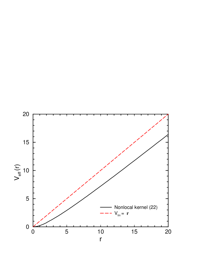
FIG. 1.: Behaviour of the effective potential, $V_{eff}(r)=\int\tilde{M}_{11}(r,x)rxdx$, as a function of $r$ (solid line). The kernel (25) and units of $\sqrt{\sigma}$ have been used. For comparison, the linear local potential $V_{lin}(r)=r$ (dashed line) is also plotted.

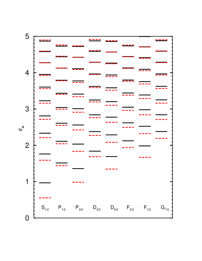
FIG. 2.: Level Structure calculated with the Dirac equation using the kernel (27) (solid line) in comparison with the predictions of the linear potential $V_{0}(r)=0.9r-1.8$ (dashed line). States carry the quantum numbers $L_{J}$, with $L,J$ being the orbital and total angular momentum.

FIG. 3.: Eigenfunctions of the ground state and the first excited state for the $S_{\frac{1}{2}}$ and $P_{\frac{1}{2}}$ channels. The solutions correspond to using the kernel (27) (solid line) and the shifted linear potential $V_{0}(r)=0.9r-1.8$ (dashed line).

Table 1. Energy eigenvalues for Eqs. (13-14) with $J=\frac{1}{2}$ and the kernels, given by Eq. (25) and Eq. (27), as compared with those of the Dirac equation for the linear local potential $V_{lin}(r)=r$.

	$V=r$		kernel (25)		kernel (27)
n	$\kappa=-1$	$\kappa=1$	$\kappa=-1$	$\kappa=1$	$\kappa=-1$	$\kappa=1$
0	1.619	2.294	0.925	1.472	0.969	1.516
1	2.603	3.031	1.719	2.056	1.765	2.113
2	3.291	3.626	2.277	2.541	2.334	2.608
3	3.855	4.138	2.740	2.964	2.809	3.042
4	4.345	4.594	3.144	3.342	3.226	3.432
5	4.784	5.008	3.507	3.685	3.603	3.790
6	5.186	5.334	3.838	4.002	3.950	4.123

Table 2. Ground state energy eigenvalue (in units of $\sqrt{\sigma}$) for Eqs. (34-35) with $\alpha_{s}=0$, 0.3 and 0.39 and quark masses $m=5~{}MeV$, $0.15~{}GeV$ and $0.2~{}GeV$ (upper, middle and lower entry) for different values of $T_{g}$, $T_{g}=0$, 0.25, 0.5 and 1 (in units of $1/{\sqrt{\sigma}}$).

Table 3. Energy eigenvalues $\bar{\Lambda}$ of the heavy–light system in the static heavy quark approximation obtained in different approaches.

Refs.	Method	$\bar{\Lambda}~{}(GeV)$
20	QCD sum rules	$>0.5$
21	QCD sum rules	$0.4\div 0.5$
24	Lattice	$0.18\pm 0.03$
22	experim.	$0.33\pm 0.11$
25	QCM	$0.35$
26	QCM	$0.5\div 0.6$
27	Rel. QCM	$0.386$
this work	Nonlin. Dirac Eq.	$0.287$

Table 4. The difference $s_{n}=|A_{n}|^{2}-|B_{n}|^{2}$ for $n=0,1,...6$, in case of the nonlocal kernels (25) and (27) and corrected for a normalized Gaussian nonlocality (52) with a range of $a$ =0.3 and $a$=0.5. For comparison the results are shown for a local linear potential $V_{lin}=r$ .

	$A_{n}^{2}-B_{n}^{2}$
n	$V=r$	kernel (25)	kernel (27)	$a$=0.3	$a$=0.5
0	0.79	0.42	0.50	0.15	0.23
1	0.51	0.21	0.34	0.04	0.12
2	0.41	0.12	0.19	0.02	0.10
3	0.35	0.10	0.16	0.02	0.09
4	0.31	0.08	0.11	0.01	0.09
5	0.27	0.07	0.11	0.01	0.08
6	0.26	0.06	0.09	0	0.07

REFERENCES

- [1] M. Creutz, Quarks, gluons, and lattices, Cambridge Univ. Press, Cambridge, 1983.
- [2] L. Del Debbio, A. Di Giacomo and Yu. A. Simonov, Phys. Lett. B332 (1994) 111.
- [3] Yu. A. Simonov, JETP Lett. 55 (1992) 627.
- [4] A. Di Giacomo, E. Meggiolaro, H. Panagopoulos, Nucl. Phys. B483 (1997) 371; Nucl. Phys. Proc. Suppl. A54 (1997) 343.
-
[5]
J. Cleymans, R. V. Gavai, E. Suhonen, Phys. Rep 130 (1986) 21.
F. Karsch, in: QCD: 20 Years Later, Zerwas P.M. and Kastrup H.A. Eds., Singapore, World Sci. 1993. -
[6]
H. G. Dosch, Phys. Lett. B190 (1987) 177.
H. G. Dosch and Yu. A. Simonov, Phys. Lett. B205 (1988) 339.
Yu. A. Simonov, Nucl. Phys. B307 (1988) 512; Yad.Fiz. 54 (1991) 192. - [7] Yu. A. Simonov, Physics – Uspekhi 39 (1996) 313.
- [8] Yu. A. Simonov, Yad.Fiz. 60 (1997) 2252; Few Body Systems, 24 (1998) 45.
-
[9]
V. S. Popov, et al. ZhETF 76 (1979) 431.
V. D. Mur and V. S. Popov, Yad.Fiz. 28 (1978) 837. - [10] I. I. Balitsky, Nucl. Phys. B254 (1985) 166.
- [11] G. Bali, HEP-LAT/9908021.
- [12] Yu. A. Simonov, in preparation.
- [13] A. Di Giacomo and H. Panagopoulos, Phys. Lett. B285 (1992) 133.
- [14] J. A. Tjon, International Conference on Quark Confinement and Hadron Spectrum, (Confinement III) Jefferson Lab, USA (1998).
- [15] V. L. Morgunov, A. V. Nefediev and Yu. A. Simonov, Phys. Lett B459 (1999) 653.
- [16] Yu. A. Simonov, Yad. Fiz. (in press); J. A. Tjon and Yu. A. Simonov, (in preparation).
- [17] Yu. A. Simonov, in: Lecture Notes in Physics, Springer, v.479, p. 139, 1996.
- [18] A. Falk, B. Grinstein and M. Luke, Nucl. Phys. B357 (1991) 185.
- [19] T. Mannel, in: Lecture Notes in Physics, Springer, v.479, p. 387, 1996.
-
[20]
I. Bigi, M. Shifman, N. C. Uraltsev and A. Vainshtein, Phys. Rev.
D52 (1995) 196; Int. J. Mod. Phys. A9 (1994) 2467;
I. Bigi, A. G. Grozin, M. Shifman, N. C. Uraltsev and A. Vainshtein, Phys. Lett. B339 (1994) 160. -
[21]
P. Ball and V. M. Braun, Phys. Rev. D49 (1994) 2472;
E. Bagan, P. Ball, V. M. Braun and V. Grosdzinsky, Phys. Lett. B342 (1995) 362. - [22] M. Gremm, A. Kapustin, Z. Ligeti and M. B. Wise, Phys. Rev. Lett. 77 (1996) 20.
- [23] A. Pineda and F. J. Yndurain, Phys. Rev. D58 (1998) 940022; preprint CERN-TH/98-402.
- [24] V. Giménez, G. Martinelli and C. T. Sachrajda, Nucl. Phys. B486 (1997) 227; Phys. Lett. B393 (1997) 124.
- [25] F. De Fazio, Mod. Phys. Lett. A11 (1996) 2693.
- [26] D. S. Hwang, C. S. Kim, W. Namgung, Phys. Rev. D54 (1996) 5620; Phys. Lett. B406 (1997) 117.
- [27] S. Simula, HEP-PH/9709247.