Discovery and Identification of Extra Gauge Bosons in $e^{+}e^{-}\to\nu\bar{\nu}\gamma$

Abstract

We examine the sensitivity of the process $e^{+}e^{-}\rightarrow\nu\bar{\nu}\gamma$ to extra gauge bosons, $Z^{\prime}$ and $W^{\prime}$, which arise in various extensions of the standard model. The process is found to be sensitive to $W^{\prime}$ masses up to several TeV, depending on the model, the center of mass energy, and the assumed integrated luminosity. If extra gauge bosons were discovered first in other experiments, the process could also be used to measure $Z^{\prime}\nu\bar{\nu}$ and $W^{\prime}$ couplings. This measurement would provide information that could be used to unravel the underlying theory, complementary to measurements at the Large Hadron Collider.

I Introduction

Extra gauge bosons, both charged ($W^{\prime}$) and/or neutral ($Z^{\prime}$), arise in many models of physics beyond the Standard Model (SM) [1, 2]. Examples include extended gauge theories such as grand unified theories [3] and Left-Right symmetric models [4] along with the corresponding supersymmetric models, and other models such as those with finite size extra dimensions [5]. To elucidate what physics lies beyond the Standard Model it is necessary to search for manifestations of that new physics with respect to the predicted particle content, both fermions and extra gauge bosons. Such searches are a feature of ongoing collider experiments and the focus of future experiments. The discovery of new particles would provide definitive evidence for physics beyond the Standard Model and, in particular, the discovery of new gauge bosons would indicate that the standard model gauge group was in need of extension. There is a considerable literature on $Z^{\prime}$ searches. In this paper we concentrate on $W^{\prime}$ searches, for which much less work has been done.

Limits have been placed on the existence of new gauge bosons through indirect searches based on the deviations from the SM they would produce in precision electroweak measurements. For instance, indirect limits from $\mu$-decay constrain the LRM $W^{\prime}$ to $M_{W_{LR}^{\prime}}\gtrsim 550$ GeV [6]. A more severe constraint arises from $K_{L}-K_{S}$ mass-splitting which gives $M_{W_{LR}^{\prime}}\gtrsim 1.6$ TeV [7]. In obtaining the above limits, it was assumed that the coupling constants of the two $SU(2)$ gauge groups are equal.

New gauge boson searches at hadron colliders consider their direct production via the Drell-Yan process and their subsequent decay to lepton pairs. For $W^{\prime}$ bosons, decays to hadronic jets are sometimes also considered. The present bounds on neutral gauge bosons, $Z^{\prime}$’s, from the CDF and D0 collaborations at the Tevatron $p\bar{p}$ collider at Fermilab are $M_{Z^{\prime}}>590-690$ GeV with the exact value depending on the specific model [7]. For $W^{\prime}$’s the limits are $M_{W^{\prime}}>300-720$ GeV; again the limits depend on the details of the model [7]. The search reach is expected to increase by $\sim 300$ GeV with 1 fb^-1 of luminosity [2, 8]. The Large Hadron Collider is expected to be able to discover $Z^{\prime}$’s up to masses of 4-5 TeV [2, 8] and $W^{\prime}$’s up to masses of $\sim 5.9$ TeV [8]. The $W^{\prime}$ limits assume SM strength couplings and decay into a light stable neutrino which is registered in the detector as missing $E_{T}$. They can be seriously degraded by loosening the assumptions in the model.

In addition, one can place limits on new gauge bosons by looking for deviations from SM expectations for observables measured at $ep$ and $e^{+}e^{-}$ colliders.

Searches for new gauge bosons at $e^{+}e^{-}$ colliders are kinematically limited by the available center-of-mass energy so that one searches for indirect effects of extra gauge bosons in cross sections and asymmetries for $\sqrt{s}<M_{V^{\prime}}$. There is a considerable body of work on $Z^{\prime}$ searches at $e^{+}e^{-}$ colliders and, although the discovery limits are very model dependent, they lie in the general range of 2-5 TeV for $\sqrt{s}=500$ GeV with 50 fb^-1 luminosity [2].

In contrast to the $Z^{\prime}$ case, there are virtually no studies of indirect searches for $W^{\prime}$ bosons at $e^{+}e^{-}$ colliders. Recently, Hewett suggested that the reaction $e^{+}e^{-}\to\nu\bar{\nu}\gamma$ would be sensitive to $W^{\prime}$’s with masses greater than $\sqrt{s}$ [9]. In the Standard Model, this process proceeds through $s$-channel $Z$ and $t$-channel $W$ exchange with the photon being radiated from every possible charged particle. In extended gauge models the process is modified by both $s$-channel $Z^{\prime}$ and $t$-channel $W^{\prime}$ exchange. In this paper, we examine this process for various extended electroweak models. The first model we consider is the Left-Right symmetric model [4] based on the gauge group $SU(3)_{C}\times SU(2)_{L}\times SU(2)_{R}\times U(1)_{B-L}$ which has right-handed charged currents. The second model we consider is the Un-Unified model [10, 11] which is based on the gauge group $SU(2)_{q}\times SU(2)_{l}\times U(1)_{Y}$ where the quarks and leptons each transform under their own $SU(2)$. The final type of model, which has received considerable interest lately, contains the Kaluza-Klein excitations of the SM gauge bosons which are a possible consequence of theories with large extra dimensions [5]. The models under consideration are described in more detail in Section II. Additionally, we study discovery limits for various combinations of $W^{\prime}$ and $Z^{\prime}$ bosons with SM couplings. Although these are not realistic models, they have been adopted as benchmarks to compare the discovery reach of different processes.

We will find that, while the process $e^{+}e^{-}\to\nu\bar{\nu}\gamma$ can indeed extend the discovery reach for $W^{\prime}$’s significantly beyond $\sqrt{s}$, with the exact limit depending on the specific model, it is not in general competitive with limits obtainable at the LHC. However, if extra gauge bosons are discovered which are not overly massive, the process considered here could be used to measure their couplings. This would be crucial for determining the origins of the $Z^{\prime}$ or $W^{\prime}$. As such, it would play an important complementary role to the LHC studies.

In the next section we review the relevant details of the various models that we use in our calculations. In Section III, we describe the details of our calculations. The resulting $W^{\prime}$ discovery limits and projected sensitivities for $W^{\prime}$ couplings and $Z^{\prime}\nu\bar{\nu}$ couplings are given in Section IV. We conclude with some final comments.

II Models

In this section, we describe the models considered in our investigation. The so-called Sequential Standard Model (SSM) includes additional weak gauge bosons of higher mass, with SM couplings. This is a rather arbitrary scenario which we include only as a benchmark. Since our emphasis here is on extra $W$’s, we consider a SSM with a $W^{\prime}$ only, which we refer to as SSM($W^{\prime}$), and a SSM with both $W^{\prime}$ and $Z^{\prime}$, denoted by SSM($W^{\prime}+Z^{\prime}$). In the latter, we will take $M_{Z^{\prime}}=M_{W^{\prime}}$ for simplicity.

The general Left-Right symmetric model (LRM) [4] is based on the extended electroweak gauge group $SU(2)_{L}\times SU(2)_{R}\times U(1)_{B-L}$. Left-handed fermion fields transform as doublets under $SU(2)_{L}$ and as singlets under $SU(2)_{R}$. The reverse is true for right-handed fermions. A right-handed neutrino is included in the fermion content. The model is parametrized by the ratio of the coupling constants of the two $SU(2)$ gauge groups, which we denote as $\kappa=g_{R}/g_{L}$. This parameter is allowed to vary here in the approximate range $0.55\lesssim\kappa\lesssim 2.0$ [9, 13, 14]. The lower bound on $\kappa$ arises from the condition $\sin^{2}\theta_{W}\leq\frac{\kappa^{2}}{1+\kappa^{2}}$ (or, equivalently, $\kappa^{2}\geq\tan^{2}\theta_{W}$), which expresses the positivity of a ratio of squared couplings. In principle, $\kappa$ is restricted to be less than 1 based on symmetry breaking scenarios and coupling constant evolution arguments. However, it is conceivable that this bound may be violated in some Grand Unified Theory so we take a phenomenological approach and loosen this upper bound [9, 14].

Additionally, a parameter, $\rho$, describes the Higgs content of the model. If only Higgs doublets are used to break the gauge symmetry to $U(1)_{em}$, $\rho$ is 1. For Higgs triplets, $\rho$ is 2. A combination of doublets and triplets leads to an intermediate value of $\rho$ between 1 and 2 [15]. We will use $\rho=1$, corresponding to Higgs doublets.

In the LRM, there is a relationship between the $Z^{\prime}$ and $W^{\prime}$ masses, as follows:

$$\frac{M^{2}_{Z^{\prime}}}{M^{2}_{W^{\prime}}}=\frac{\rho\kappa^{2}}{\kappa^{2}-\tan^{2}\theta_{W}}.$$ (1)

The couplings of the extra gauge bosons relevant to our calculation can be read from the following parts of the Lagrangian.

$${\cal L}_{LR} = \frac{e\kappa}{\sqrt{2}s_{W}}W^{\prime+}_{\mu}\bar{\nu}_{R}\gamma^{\mu}e_{R}+\frac{e}{2s_{W}c^{2}_{W}\sqrt{\kappa^{2}-t^{2}_{W}}}Z^{\prime}_{\mu}\left[\bar{l}\gamma^{\mu}(1-\gamma_{5})s^{2}_{W}(T_{3L}-Q_{em})l\right.$$ (3)

$$\left.+\bar{l}\gamma^{\mu}(1+\gamma_{5})(\kappa^{2}c^{2}_{W}T_{3R}-s^{2}_{W}Q_{em})l\right]+h.c.$$

where $e_{R}=\frac{1}{2}(1+\gamma_{5})e$ denotes a right-handed electron field. Note that we neglect two angles, usually denoted as $\xi$ and $\zeta$, which parametrize the $Z-Z^{\prime}$ and $W-W^{\prime}$ mixings, respectively. Limits on these angles are rather severe so this is justified [16, 17]. Neglect of these angles implies SM couplings for the $Z$ and $W$. Additionally, we assume light Dirac-type neutrinos.

The Un-Unified model (UUM) [10, 11] employs the alternative electroweak gauge symmetry $SU(2)_{q}\times SU(2)_{l}\times U(1)_{Y}$ with left-handed quarks and leptons transforming as doublets under their respective $SU(2)$ groups. All the right-handed fields transform as singlets under both $SU(2)$ groups. The UUM may be parametrized by an angle $\phi$, which represents the mixing of the charged gauge bosons of the two $SU(2)$ groups, and by a ratio $x=(u/v)^{2}$, where $u$ and $v$ are the vacuum expectation values of the scalar multiplets which break the symmetry to $U(1)_{em}$. The existing constraint on $\phi$ is $0.24\lesssim\sin\phi\lesssim 0.99$, based on the validity of perturbation theory. For $x/\sin^{2}\phi\gg 1$, the $Z^{\prime}$ mass is approximately equal to that of the $W^{\prime}$ and the parameter $x$ may be replaced by $M_{W^{\prime}}$. The lepton couplings of interest to us here arise from the following part of the Lagrangian.

$${\cal L}_{UU} = -\frac{e}{2s_{W}}\frac{s_{\phi}}{c_{\phi}}\left[\sqrt{2}W^{\prime+}_{\mu}\bar{\nu}\gamma^{\mu}l_{L}+Z^{\prime}_{\mu}(\bar{\nu}\gamma^{\mu}\nu_{L}-\bar{l}\gamma^{\mu}l_{L})\right]+h.c.$$ (4)

As expected, the fermion couplings to the additional gauge bosons are all left-handed in the UUM. Additional fermions must also be included in order to cancel anomalies. This is rather difficult to do without generating flavour changing neutral currents and some considerations of this problem lead to rather high lower bounds on the $Z^{\prime}$ mass of about 1.4 TeV [11]. However, lower $Z^{\prime}$ and $W^{\prime}$ masses may be allowed in other scenarios; hence we take a phenomenological approach in this investigation.

Finally, we consider the consequences of models which have been of considerable interest lately, those containing large extra dimensions [5]. In particular, we consider an extension of the SM to 5-dimensions (5DSM) [12]. The presence of an extra dimension of size $R\sim$ TeV^-1 may imply an infinite tower of Kaluza-Klein (KK) excitations of the SM gauge bosons. The mass of the excitations is associated with the compactification scale of the extra dimension as $nM_{c}$ ($n=1,...,\infty$), where $M_{c}=1/R$. The properties of and relationships among electroweak observables are modified by the presence of these KK towers. We treat this possibility in a manner similar to the other models described above; that is, we include in our process the exchange of a $W^{\prime}$ and $Z^{\prime}$ corresponding to the first KK excitations. The model can be parametrized by an angle $\beta$ which is correlated with the properties of its Higgs sector, which includes two doublets; for $\sin\beta\equiv s_{\beta}=0$, the SM Higgs may propagate in all 5-dimensions (the bulk) while for $s_{\beta}=1$, it is confined to the 4-dimensional boundary. In terms of this parameter, the physical masses of the lightest electroweak gauge bosons (corresponding to the experimentally measured masses) are given, to first order in $M^{2}_{W}/M^{2}_{c}$, as

$$M^{(ph)2}_{W} = M^{2}_{W}\left[1-s^{4}_{\beta}\frac{\pi^{2}}{3}\frac{M^{2}_{W}}{M^{2}_{c}}\right]$$ (5)

$$M^{(ph)2}_{Z} = M^{2}_{Z}\left[1-s^{4}_{\beta}\frac{\pi^{2}}{3}\frac{M^{2}_{Z}}{M^{2}_{c}}\right]$$ (6)

where $M^{2}_{W}=g^{2}v^{2}/2$, as usual.The gauge couplings of the physical $W$ and $Z$ are also modified by a term of order $M^{2}_{V}/M^{2}_{c}$. Global analyses of electroweak parameters put a lower limit on $M_{c}$ of about 2.5 TeV so this is a very small effect. We will therefore neglect it and thus eliminate $s_{\beta}$ as a parameter. On the other hand, the fermion coupling of the first KK excitations, $W^{\prime}$ and $Z^{\prime}$, each of mass $M_{V^{\prime}}=M_{c}$, is enhanced by a factor of $\sqrt{2}$. Hence our consideration of the 5DSM amounts to including a $W^{\prime}$ and a $Z^{\prime}$, of equal mass, each coupling as in the SM apart from an extra factor of $\sqrt{2}$.

III Calculation

The process under consideration is

$$e^{-}(p_{-})+e^{+}(p_{+})\rightarrow\gamma(k)+\nu(q_{-})+\bar{\nu}(q_{+})\,\,.$$ (7)

The relevant Feynman diagrams are given in Fig. 1. The kinematic observables of interest are the photon’s energy, $E_{\gamma}$, and its angle relative to the incident electron, $\theta_{\gamma}$, both defined in the $e^{+}e^{-}$ center-of-mass frame. The invariant mass of the $\nu\bar{\nu}$ pair, $M_{\nu\bar{\nu}}$, and $E_{\gamma}$ are related via

$$E_{\gamma}=\frac{\sqrt{s}}{2}\left(1-\frac{M_{\nu\bar{\nu}}^{2}}{s}\right),$$ (8)

where $s=(p_{+}+p_{-})^{2}$.

Let ${\cal M}$ denote the sum of the amplitudes shown in Fig. 1, over a given number of $Z^{\prime}$’s and $W^{\prime}$’s. The doubly differential cross section is related to $|{\cal M}|^{2}$ via

$$\frac{d\sigma}{dE_{\gamma}d\cos\theta_{\gamma}}=\frac{E_{\gamma}}{2s}\frac{1}{(4\pi)^{4}}\int_{0}^{\pi}d\theta\sin\theta\int_{0}^{2\pi}d\varphi|{\cal M}|^{2},$$ (9)

where $\theta$ and $\varphi$ are the polar and azimuthal angles, respectively, of $q_{+}$ in a frame where $q_{+}$ and $q_{-}$ are back-to-back. The explicit momentum parametrizations are given in the Appendix.

Two approaches to determining $|{\cal M}|^{2}$ are possible. One can determine ${\cal M}$ analytically, using spinor techniques [18, 19] for instance, then square it numerically or one can find $|{\cal M}|^{2}$ analytically. We have followed both approaches, which provides an independent check. Obtaining $|{\cal M}|^{2}$ analytically has been done both via the trace method, using the symbolic manipulation program FORM [20], and by squaring the helicity amplitudes and summing over the final state helicities. The latter approach leads to a rather compact result which we present below.

In order to present $|{\cal M}|^{2}$, we define the following kinematic variables. We follow the notation of [21], where the SM contribution for this process was calculated:

$$\begin{array}[]{rrlrl}&s=&(p_{+}+p_{-})^{2},&s^{\prime}=&(q_{+}+q_{-})^{2},\\ &t=&(p_{+}-q_{+})^{2},&t^{\prime}=&(p_{-}-q_{-})^{2},\\ &u=&(p_{+}-q_{-})^{2},&u^{\prime}=&(p_{-}-q_{+})^{2},\\ &k_{\pm}=&2p_{\pm}\cdot k,&k^{\prime}_{\pm}=&2q_{\pm}\cdot k,\\ Z_{i}=s^{\prime}-M_{Z_{i}^{2}}+iM_{Z_{i}}\Gamma_{Z_{i}},&W_{i}=&t-M_{W_{i}^{2}},&W_{i}^{\prime}=&t^{\prime}-M_{W_{i}^{2}}.\end{array}$$ (10)

The decay width of the extra neutral gauge boson, $\Gamma_{Z_{i}}$, into fermion- antifermion pairs is calculated in each of the models we consider. We include the one-loop QED, three-loop QCD and $O(M_{t}^{2}/M_{Z^{\prime}}^{2})$ corrections, although their effect on the cross section is negligible. In the following, we denote generalized couplings as may be inferred from the vertices

$$Z_{i}f\bar{f} = \frac{ig}{2c_{W}}\gamma^{\mu}\left(\frac{1-\gamma_{5}}{2}\,\,a_{Z_{i}}^{f}+\frac{1+\gamma_{5}}{2}\,\,b_{Z_{i}}^{f}\right)$$ (11)

$$W_{i}l\nu = \frac{ig}{\sqrt{2}}\gamma^{\mu}\left(\frac{1-\gamma_{5}}{2}\,\,a_{W_{i}}+\frac{1+\gamma_{5}}{2}\,\,b_{W_{i}}\right).$$ (12)

Thus, in the SM, $a^{e}_{Z_{1}}=2s_{W}^{2}-1$, $b^{e}_{Z_{1}}=2s_{W}^{2}$, $a^{\nu}_{Z_{1}}=1$, $b^{\nu}_{Z_{1}}=0$, $a_{W_{1}}=1$, and $b_{W_{1}}=0$.

It is only necessary to present the unpolarized squared amplitude as the individual polarized contributions may be inferred from the coupling structure. The spin-averaged unpolarized $|{\cal M}|^{2}$ is given by:

$$|{\cal M}|^{2}_{\rm unp} = \frac{(4\pi)^{3}\alpha^{3}}{8s_{W}^{4}k_{+}k_{-}}\left\{\mbox{\raisebox{17.22217pt}{}}\right.\frac{3s^{\prime}}{c_{W}^{4}}\sum_{\stackrel{{\scriptstyle\scriptstyle i=1,nz}}{{j=i,nz}}}Z_{ij}[(a^{e}_{Z_{i}}a^{e}_{Z_{j}}a^{\nu}_{Z_{i}}a^{\nu}_{Z_{j}}+b^{e}_{Z_{i}}b^{e}_{Z_{j}}b^{\nu}_{Z_{i}}b^{\nu}_{Z_{j}})(u^{2}+u^{\prime 2})$$ (17)

$$\,\,\,\,\,\,\,\,\,\,\,\,\,\,\,\,\,\,\,\,\,\,\,\,\,\,\,\,\,\,\,\,\,\,\,\,\,\,\,\,\,\,\,\,\,\,\,\,\,\,\,\,\,\,\,\,\,\,\,\,\,\,\,\,\,\,\,+(a^{e}_{Z_{i}}a^{e}_{Z_{j}}b^{\nu}_{Z_{i}}b^{\nu}_{Z_{j}}+b^{e}_{Z_{i}}b^{e}_{Z_{j}}a^{\nu}_{Z_{i}}a^{\nu}_{Z_{j}})(t^{2}+t^{\prime 2})]$$

$$+\frac{4}{s^{\prime}}\sum_{\stackrel{{\scriptstyle\scriptstyle i=1,nw}}{{j=i,nw}}}W_{ij}[(a^{2}_{W_{i}}a^{2}_{W_{j}}+b^{2}_{W_{i}}b^{2}_{W_{j}})(u^{2}+u^{\prime 2})+2a_{W_{i}}a_{W_{j}}b_{W_{i}}b_{W_{j}}(s^{2}+s^{\prime 2})]$$

$$+\frac{4}{c^{2}_{W}}\sum_{\stackrel{{\scriptstyle\scriptstyle i=1,nw}}{{j=1,nz}}}[\left(WZ\right)_{ij}(u^{2}a^{2}_{W_{i}}a^{e}_{Z_{j}}a^{\nu}_{Z_{j}}+u^{\prime 2}b^{2}_{W_{i}}b^{e}_{Z_{j}}b^{\nu}_{Z_{j}})$$

$$\,\,\,\,\,\,\,\,\,\,\,\,\,\,\,\,\,\,\,\,\,\,\,\,\,\,\,+\left(WZ\right)^{\prime}_{ij}(u^{\prime 2}a^{2}_{W_{i}}a^{e}_{Z_{j}}a^{\nu}_{Z_{j}}+u^{2}b^{2}_{W_{i}}b^{e}_{Z_{j}}b^{\nu}_{Z_{j}})]\left.\mbox{\raisebox{17.22217pt}{}}\right\},$$

where

$$\begin{array}[]{rclrcl}Z_{ij}&=&{\displaystyle{\rm Re}\left(\frac{2-\delta_{ij}}{Z_{i}Z^{*}_{j}}\right)},&W_{ij}&=&(2-\delta_{ij}){\rm Re}(F_{W_{i}}F^{*}_{W_{j}}),\,\,\,\,\,\,\left(WZ\right)_{ij}={\displaystyle{\rm Re}\left(\frac{F_{W_{i}}}{Z_{j}}\right)},\\ &&&&&\\ \left(WZ\right)^{\prime}_{ij}&=&{\displaystyle{\rm Re}\left(\frac{F_{W_{i}}}{Z^{*}_{j}}\right)},&F_{W_{i}}&=&{\displaystyle\frac{s^{\prime}}{W^{\prime}_{i}}-\frac{s^{\prime}k_{+}-tk^{\prime}_{-}+uk^{\prime}_{+}-4i\varepsilon(q_{+}q_{-}p_{+}k)}{2W_{i}W^{\prime}_{i}}},\end{array}$$ (18)

using the notation $\varepsilon(p_{1}p_{2}p_{3}p_{4})=\varepsilon_{\mu\nu\rho\sigma}p_{1}^{\mu}p_{2}^{\nu}p_{3}^{\rho}p_{4}^{\sigma}$, where $\varepsilon_{\mu\nu\rho\sigma}$ is the completely antisymmetric Levi-Civita tensor and $\varepsilon_{0123}=1$. In Eq. (17) we have assumed lepton universality with regards to the $Z^{\prime}\nu\bar{\nu}$ couplings. Although it may not be immediately apparent, the contribution to the cross section from the state where the $e^{-}$ and $e^{+}$ are both left-handed is equal to the contribution from the state where they are both right-handed and the sum is given by the term in Eq. (17) proportional to $a_{W_{i}}a_{W_{j}}b_{W_{i}}b_{W_{j}}$.

A relation which was quite useful in simplifying $|{\cal M}|^{2}$ is

$$\frac{s^{\prime}}{W^{\prime}_{i}}-\frac{s^{\prime}k_{+}-tk^{\prime}_{-}+uk^{\prime}_{+}-4i\varepsilon(q_{+}q_{-}p_{+}k)}{2W_{i}W^{\prime}_{i}}=\frac{s^{\prime}}{W_{i}}-\frac{s^{\prime}k_{-}-t^{\prime}k^{\prime}_{+}+u^{\prime}k^{\prime}_{-}-4i\varepsilon(q_{-}q_{+}p_{-}k)}{2W_{i}W^{\prime}_{i}}.$$ (19)

In the SM limit, Eq. (17) agrees with the expression given in [21] after correcting for the known missing factors of $1/s^{\prime}$ in [21] required on dimensional grounds.

The calculation of $d\sigma/dE_{\gamma}d\cos\theta_{\gamma}$ may be performed analytically or numerically. We have followed both approaches and verified numerical agreement. Further checks were performed using the program CompHEP [22].

IV Results

Before discussing the discovery limits obtained in the various models, we present the total cross sections and the differential cross sections $d\sigma/dE_{\gamma}$ and $d\sigma/d\cos\theta_{\gamma}$. In doing so, all the essential features are illustrated. We take the SM inputs $M_{W}=80.33$ GeV, $M_{Z}=91.187$ GeV, $\sin^{2}\theta_{W}=0.23124$, $\alpha=1/128$, $\Gamma_{Z}=2.49$ GeV [7]. Since we work only to leading order in $|{\cal M}|^{2}$, there is some arbitrariness in what to use for the above input, in particular $\sin^{2}\theta_{W}$.

Kinematically, the maximum allowed value for $E_{\gamma}$ is $\sqrt{s}/2$. In addition, to take into account detector acceptance, $E_{\gamma}$ and $\theta_{\gamma}$ have been restricted to the ranges

$$E_{\gamma}\geq 10\,\,{\rm GeV},\hskip 28.45274pt10^{0}\leq\theta_{\gamma}\leq 170^{0}.$$ (20)

The cuts also serve to remove the singularities which arise when the emitted photon is soft or collinear with the beam. Further, we restrict the photon’s transverse momentum to

$$p_{T}^{\gamma}>\frac{\sqrt{s}\sin\theta_{\gamma}\sin\theta_{v}}{\sin\theta_{\gamma}+\sin\theta_{v}},$$ (21)

where $\theta_{v}$ is the minimum angle down to which the veto detectors may observe electrons or positrons. We take $\theta_{v}=25$ mrad. This cut has the effect of removing the largest background to our process, namely radiative Bhabha-scattering where the scattered $e^{+}$ and $e^{-}$ go undetected down the beam pipe.

This study was performed in leading order, but QED corrections to $e^{+}e^{-}\rightarrow\nu\bar{\nu}\gamma$ must be taken into account in a precision analysis of real data. They have been known to $O(\alpha)$ for some time [21]. See [23] for a short review of and further references to higher order QED corrections, and [24] for a description of a related MC generator. Since our aim is to determine the statistical power of the process in discovering $W^{\prime}$’s, there is no need to include in this study the radiative corrections which will only marginally influence the number of events. Complete consistency at NLO, however, would require determination of the bremsstrahlung corrections to the generalized expression (17) and corresponding loop graphs.

As well, we do not explicitly take into account any higher order backgrounds. A background, which cannot be suppressed, comes from the reaction $e^{+}e^{-}\rightarrow\nu\bar{\nu}\nu^{\prime}\bar{\nu}^{\prime}\gamma$. The authors of [25] have provided the following cross sections of relevance here: $\sigma(e^{+}e^{-}\rightarrow\nu_{e}\bar{\nu}_{e}\nu_{e}\bar{\nu}_{e}\gamma)\equiv\sigma_{eeee}=6.65(2)\,{\rm fb},\ \ \sigma_{ee\mu\mu}=7.79(2)\,{\rm fb},\ \ \sigma_{\mu\mu\mu\mu}=0.690(2)\,{\rm fb}\ \$ and  $\sigma_{\mu\mu\tau\tau}=1.383(3)\,{\rm fb}$. These results are for the same conditions as in Table 1 of [25] but for $\sqrt{s}=500\,{\rm GeV}$. The cuts used in obtaining the above numbers differ from ours. Nonetheless, these cross sections give an idea of the magnitude of the background. Assuming lepton universality, the total cross section is $25\,{\rm fb}$ for the process $e^{+}e^{-}\rightarrow\nu\bar{\nu}\nu^{\prime}\bar{\nu}^{\prime}\gamma$. Imposing our $p_{T}^{\gamma}$ cut will suppress it even further. This background must be included in an “$e^{+}e^{-}\rightarrow\gamma$ + nothing” analysis of real data. We expect that the cross sections of $e^{+}e^{-}\rightarrow\nu\bar{\nu}\nu^{\prime}\bar{\nu}^{\prime}\gamma\gamma$ and of $e^{+}e^{-}\rightarrow\nu\bar{\nu}\nu^{\prime}\bar{\nu}^{\prime}\nu^{\prime\prime}\bar{\nu}^{\prime\prime}\gamma$ are so small that they need not be taken into account in the analysis.

The errors generated from the subtraction of the above backgrounds form part of the systematic error. As the backgrounds themselves are much smaller than the signal, though comparable to the new physics effect, we expect that the error in the SM prediction of the backgrounds would be much smaller than the systematic errors arising from detector and beam uncertainties. We shall return to the issue of systematics in connection with their influence on the discovery limits presented in the next section.

We have calculated three distinct total cross sections: unpolarized: $\sigma$, for left-handed $e^{-}$: $\sigma_{L}$, and for right-handed $e^{-}$: $\sigma_{R}$. Fig. 2 shows all three plotted versus $\sqrt{s}$, with $\sigma_{L}$ and $\sigma_{R}$ calculated using 100% beam polarization. Results are shown for the SM, LRM ($\rho=\kappa=1$), UUM ($\sin\phi=0.6$), SSM($W^{\prime}$), SSM($W^{\prime}+Z^{\prime}$) and KK model, with $M_{W^{\prime}}=750$ GeV in each case. These mass and coupling parameter choices are rather arbitrary, made to illustrate general behaviour. It is worth noting at this point that in the UUM and SSM($W^{\prime}+Z^{\prime}$), the correction to the SM cross section changes sign as $\sqrt{s}$ is varied. This arises, for certain $\sqrt{s}$ and $M_{W^{\prime}}$, due to a negative interference term between the SM and $Z^{\prime}/W^{\prime}$ diagrams in these models.

It is clear from the presence of the peaks in Fig. 2 that we are also probing $Z^{\prime}$’s, in those models which include them. (There is also a very sharp peak at lower $\sqrt{s}$, off the plot, due to the SM $Z$.) The $Z^{\prime}$ peaks generally occur for $\sqrt{s}$ slightly above the $Z^{\prime}$ mass since the photon carries away some of the energy. At very high energies, the SM $Z$ contribution is negligible. Further, by using a right-handed $e^{-}$ beam, we can reduce the SM $W$ contribution (depending on the degree of polarization). Then we directly probe the $W^{\prime}$ (and $Z^{\prime}$) in the LRM, while in the SSM($W^{\prime}+Z^{\prime}$) and KK model, we probe only the $Z^{\prime}$. The latter two models as well as the two remaining models all require some component of left-handed polarization to probe the $W^{\prime}$. The above features are borne out in Fig. 2.

In order to see which regions of $E_{\gamma}$ are most sensitive to the new physics, we plot for left- and right-handed electron beams respectively, in Figs. 3(a) and 4(a) $d\sigma/dE_{\gamma}$ versus $E_{\gamma}$ and in Figs. 3(b) and 4(b) the deviation from the SM result divided by the square root of the predicted cross section versus $E_{\gamma}$. We show results for $\sqrt{s}=500$ GeV with 100% $e^{-}$ beam polarization in these figures.

First, we note the shape of $d\sigma/dE_{\gamma}$ in Figs 3(a) and 4(a). For left-handed electrons, the bulk of the cross section comes from the low $E_{\gamma}$ region; the reduction at very low $E_{\gamma}$ is due to the $p_{T}^{\gamma}$ cut and the sharp peak at $E_{\gamma}\simeq 240$ GeV is due to the radiative return to the $Z$ pole. For 100% right polarized electrons, the cross section is rather flat in the low to moderate $E_{\gamma}$ region, then increases as a result of the $Z$ peak at high $E_{\gamma}$. On the other hand, since the right-handed cross section is two orders of magnitude smaller than the left-handed cross section away from the $Z$ peak, any realistic degree of polarization (i.e. 90%) will lead to a large contribution from $\sigma_{L}$ to the low $E_{\gamma}$ region. In general, there can also be a peak due to a $Z^{\prime}$ for $M_{Z^{\prime}}<\sqrt{s}$ which occurs at

$$E_{\gamma}^{\rm peak}=\frac{\sqrt{s}}{2}\left(1-\frac{M_{Z^{\prime}}^{2}}{s}\right)$$ (22)

in analogy with the SM $Z$.

Most important, however, is the relative statistical significance, shown in Figs. 3(b) and 4(b). In both the left- and right-handed cases, the low $E_{\gamma}$ region is the most sensitive to the new physics. There are two reasons for this. First, for left-handed electrons, the cross section is largest at low $E_{\gamma}$, as mentioned above. Second, the lower $E_{\gamma}$, the higher the mass probed in the $Z^{\prime}$ propagator via Eq. (8). The relative effect is even larger when combining the $\chi^{2}$’s from the different bins, since it is the squares of the plotted quantities which will enter. Overall, the KK model leads to the most statistically significant deviations, except for the 100% left polarized case where the SSM($W^{\prime}$) exhibits the largest deviation. We can also see clearly how the sign of the deviation from the SM depends on the beam polarization. For the KK model and SSM($W^{\prime}+Z^{\prime}$), we observe a negative deviation with right-handed polarization, implying a negative $Z^{\prime}$ contribution, versus a positive overall contribution coming from the left-handed channel. Clearly, interference effects will make probing $W^{\prime}$’s nontrivial. We shall return to this point in the next section.

In Figs. 5 and 6 we plot the analogous quantities relevant to $d\sigma/d\cos\theta_{\gamma}$, versus $\cos\theta_{\gamma}$. We note that both $d\sigma/d\cos\theta_{\gamma}$ and the relative statistical significance are peaked in the forward and backward directions and both are very nearly symmetric in $\cos\theta_{\gamma}$. The latter implies that the forward-backward asymmetry will be small and, therefore, the deviation from the SM forward-backward asymmetry will also be small, at least in absolute magnitude. We therefore do not expect the forward-backward asymmetry to serve as a useful probe of the new physics, which is confirmed by explicit calculation. An important observation is that our $p_{T}^{\gamma}$ cut, while eliminating a large background, has also eliminated much of our signal (both from the small angle and soft events) which was appreciably stronger prior to the cut. A more detailed study, including a detector simulation, would be required to determine whether the background could be accurately subtracted with a looser $p_{T}^{\gamma}$ cut.

A Discovery Limits for $W^{\prime}$’s

The best discovery limits were in general obtained using the observable $d\sigma/dE_{\gamma}$, combined with beam polarization, while $d\sigma/d\cos\theta_{\gamma}$ was less sensitive. Comparable or equal limits were obtained using the total cross section, with an additional cut on the energy to eliminate the $Z$ pole radiative return events:

$$E_{\gamma}^{\rm max}=\frac{\sqrt{s}}{2}\left(1-\frac{M^{2}_{Z}}{s}\right)-6\Gamma_{Z}.$$ (23)

As can be seen from Figs. 3(b) and 4(b), the $Z$ pole region is quite insensitive to new physics. In the cases that $d\sigma/dE_{\gamma}$ provided a better limit than the total cross section, the improvement was of order 50 GeV. However, the $\chi^{2}$ obtained using the total cross section is a somewhat less stable function of $M_{W^{\prime}}$ as the sign of the deviation from the SM cross section may change with $M_{W^{\prime}}$ leading to isolated regions of insensitivity at low $M_{W^{\prime}}$. Also, when systematic errors are included, the limits obtained using $d\sigma/dE_{\gamma}$ are affected much less than those obtained using the total cross section.

Substantially weaker limits were obtained using the left-right asymmetry,

$$A_{LR}=\frac{\sigma_{L}-\sigma_{R}}{\sigma_{L}+\sigma_{R}},$$ (24)

even when including systematic errors only one half those used in the $d\sigma/dE_{\gamma}$ calculation (since one expects some cancellation of errors between the numerator and denominator in $A_{LR}$). As expected from the discussion of the previous section, the forward-backward asymmetry, $A_{FB}$, was quite insensitive to the new physics. In light of the above, we restrict the remaining discussion to limits obtained using $d\sigma/dE_{\gamma}$ as an observable.

In obtaining the $\chi^{2}$ for $d\sigma/dE_{\gamma}$, we used 10 equal sized energy bins in the range $E_{\gamma}^{\rm min}<E_{\gamma}<E_{\gamma}^{\rm max}$, where $E_{\gamma}^{\rm min}$ follows from the $p_{T}^{\gamma}$ cut Eq. (21):

$$E_{\gamma}^{\rm min}=\frac{\sqrt{s}\sin\theta_{v}}{1+\sin\theta_{v}},$$ (25)

which supersedes the acceptance cut of Eq. (20). We have

$$\chi^{2}=\sum_{\rm bins}\left(\frac{d\sigma/dE_{\gamma}-d\sigma/dE_{\gamma,{\rm SM}}}{\delta d\sigma/dE_{\gamma}}\right)^{2},$$ (26)

where $\delta d\sigma/dE_{\gamma}$ is the error on the measurement and analogous formulae hold for other observables. One sided 95% confidence level discovery limits are obtained by requiring $\chi^{2}\geq 2.69$ for discovery. Systematic errors, when included, were added in quadrature with the statistical errors.

In determining the limits for the case of polarized electron beams, we show results for the polarization state which in general has the largest sensitivity (deviation from the SM) for a given model; a right-handed $e^{-}$ beam for the LRM and a left-handed beam for all other models. We used one half the unpolarized luminosity for the polarized case, assuming equal running time in each polarization state.

The discovery limits for all five models are listed in Table I, for $\sqrt{s}=0.5$, 1.0 and 1.5 TeV, using the same input parameters as for the cross sections presented in the previous section. We show limits for both an unpolarized $e^{-}$ beam and for a 90% polarized one. For each center-of-mass energy, two luminosity scenarios are considered and we present limits obtained with and without systematic errors. Our prescription is to include a 2% systematic error per bin. This number is quite arbitrary but seems reasonable, if not conservative, considering the clean final state. In addition to detector systematics, which we expect will dominate, there are uncertainties associated with the beam luminosity and energy, which will be spread over a range. The systematic errors associated with the background subtraction should be much smaller than 2% as should be the errors in the calculation of the QED corrections. The 2% number should not be taken too seriously therefore, except to highlight the fact that a precision measurement is required to take full advantage of the large event rate.

Certain features are common to all models. With no systematic error included, we observe quite an improvement in the limits with increased luminosity. The only exception is the UUM at $\sqrt{s}$ of 1.5 TeV, where the improvement is minimal. The reason is that the $\chi^{2}$ decreases very rapidly as $M_{W^{\prime}}$ is increased in the vicinity of the limit, hence increasing the luminosity by a factor of 2.5 does little. The unusual $\sqrt{s}$ dependence can be attributed to the interference effect noted in the previous section, which results in, for example, for the UUM with $\sin\phi=0.6$ and an integrated luminosity of 500 fb^-1, a lower discovery limit at $\sqrt{s}=1.5$ TeV than at 0.5 and 1 TeV. We will return to this peculiar behaviour later in the section. When 2% systematic errors are included, the high luminosity scenario yields little improvement in the limits in any of the models, since the systematic error now dominates the statistical.

Perhaps surprising at first is the observation that 90% beam polarization does not improve the limits very much. This follows from taking into account the reduced luminosity and the fact that the left-handed component tends to dominate the unpolarized cross section by a considerable amount. On the other hand, we observed that if the polarization is pushed beyond 90%, then the right-polarized limits can increase significantly in those models in which the beyond-SM bosons have a non-zero right-handed coupling: the LRM, KK model and SSM($W^{\prime}+Z^{\prime}$). In the latter two models, it is however, the $Z^{\prime}$ which is being probed. The higher degree of polarization is required to eliminate the contamination from the much larger left-handed component. Thus, the primary advantage of beam polarization is to distinguish between models and measure the new couplings, as will be investigated in the next section.

Fig. 7 presents the $W^{\prime}$ mass discovery limits obtainable in the LRM with an unpolarized beam, plotted versus $\kappa$ for $\rho=1$ and $\sqrt{s}=$ $0.5$, 1.0, 1.5 and 2 TeV using a luminosity of 50 fb^-1 for $\sqrt{s}=0.5$ TeV and 200 fb^-1 for the higher energies. Only statistical errors are included. Depending on $\sqrt{s}$ and $\kappa$, the limits range from 0.8 to 2.8 TeV. We expect greater deviations from the SM, and hence larger limits, as $\kappa$ is increased since this increases the $W^{\prime}$ coupling strength, as can be seen from Eq. (3). The predicted dependence on $\kappa$ is generally observed, except at low $\kappa$ where we notice a moderate increase in the limits, even though the $W^{\prime}$ couplings have weakened. We attribute this effect to the $Z^{\prime}$, whose couplings are enhanced (but its mass increased) in the low $\kappa$ region. This was indicated by an appreciable improvement in the limits for low $\kappa$ and $\rho=1$ versus those obtained using $\rho=2$ and consequently a heavier $Z^{\prime}$, via Eq. (1). Fig. 8 demonstrates the improvement in bounds in the moderate to large $\kappa$ region obtained when a 90% or 100% polarized right-handed $e^{-}$ beam is used. The beam polarization picks out the LRM $W^{\prime}$ and suppresses the SM $W$. Fig. 8(a) shows that for $\kappa>1$, 90% beam polarization improves the limits. Further increasing the polarization leads to substantial improvements, even at lower $\kappa$, as demonstrated in Fig. 8(b).

The dependence of the limits in the UUM on $\sin\phi$ is shown in Fig. 9, for $\sqrt{s}=$ $0.5$, 1.0, 1.5 and 2.0 TeV, under the same running conditions as Fig. 7. Only the unpolarized case is considered as beam polarization was not beneficial. Again, only statistical errors are included. At each $\sqrt{s}$, we note that the contour defining the exclusion region as a function of $\sin\phi$ is a complicated curve. The consequence is that for $\sqrt{s}=1$ TeV, we obtain better limits over a range of $\sin\phi$ than we do for $\sqrt{s}=1.5$ and even $\sqrt{s}=2$ TeV. Essentially, this is due to the complicated interference with the SM diagrams. In general, as $\sin\phi$ increases, the UUM couplings also increase, as can be seen from Eq. (4), so that higher mass scales are probed. So, referring to Fig. 2, the peak in the cross section (due to the $Z^{\prime}$) at the scale being probed shifts to the right. But the sign of the deviation from the SM changes with $\sqrt{s}$ for fixed $M_{W^{\prime}}$ (or vice-versa) such that the UUM cross section dips below the SM over some region to the left of the peak, then goes back above it for small $\sqrt{s}$ (or large $M_{W^{\prime}}=M_{Z^{\prime}}$ for fixed $\sqrt{s}$). Hence, there is a small step in the limits near $M_{W^{\prime}}=\sqrt{s}$, corresponding to passing the rightmost crossing with the SM and another structure in the contour at some higher $M_{W^{\prime}}$ such that the leftmost crossing is situated near $\sqrt{s}$. One sees this explicitly by plotting $\chi^{2}$ versus $M_{W^{\prime}}$ for fixed $\sqrt{s}$ and $\sin\phi$ and observing a dip in the $\chi^{2}$ at relatively low $M_{W^{\prime}}$. Had we used $\sigma$ as an observable, the dip would be much more pronounced since $\sigma-\sigma_{\rm SM}$ passes through zero, but $d\sigma/dE_{\gamma}-d\sigma/dE_{\gamma,{\rm SM}}$ may differ in sign between bins, leading to a nonzero $\chi^{2}$ at the crossing points. Once $\sin\phi$ is large enough that we are probing the region to the left of the leftmost crossing, the limits shoot up in an impressive fashion as the dip in $\chi^{2}$ never goes back down to 2.69. The shape of the plot is luminosity dependent since, as pointed out earlier in this section, the degree to which increased luminosity improves the limits depends on the rate at which the $\chi^{2}$ decreases with increasing $M_{W^{\prime}}$ in the vicinity of the limit. That, in turn, varies with $\sqrt{s}$ for fixed $\sin\phi$ and with $\sin\phi$ for fixed $\sqrt{s}$.

B Constraints on Couplings

In this section, we consider constraints which can be put on the couplings of extra gauge bosons by the process $e^{+}e^{-}\rightarrow\nu\bar{\nu}\gamma$. These constraints are significant only in the case where the mass of the corresponding extra gauge boson is considerably lower than its search limit in this process. In most models, the process $e^{+}e^{-}\rightarrow f\bar{f}$ and/or searches at the LHC are more sensitive to a $Z^{\prime}$ or $W^{\prime}$ (LHC) than the process $e^{+}e^{-}\rightarrow\nu\bar{\nu}\gamma$. We assume here that a signal for an extra gauge boson has been detected by another experiment.

Given such a signal, we derive constraints (at 95% C.L.) on the couplings of extra gauge bosons. We present the constraints in terms of couplings normalized as follows relative to Eqs. (11) and (12).

$$\begin{array}[]{rlrl}L_{f}(Z)=&\frac{g}{4c_{W}}a^{f}_{Z_{i}}&\;\;\;R_{f}(Z)=&\frac{g}{4c_{W}}b^{f}_{Z_{i}}\\ L_{f}(W)=&\frac{g}{2\sqrt{2}}a_{W_{i}}&\;\;\;R_{f}(W)=&\frac{g}{2\sqrt{2}}b_{W_{i}}.\end{array}$$ (27)

The constraints correspond to

$$\chi^{2}=\sum_{i}\left(\frac{O_{i}(SM)-O_{i}(SM+Z^{\prime}+W^{\prime})}{\delta O_{i}}\right)^{2}=5.99,$$ (28)

where $O_{i}(SM)$ is the prediction for the observable $O_{i}$ in the SM, $O_{i}(SM+Z^{\prime}+W^{\prime})$ is the prediction of the extension of the SM and $\delta O_{i}$ is the expected experimental error. The index $i$ corresponds to different observables such as $\sigma$ and $A_{LR}$.

Our assumptions concerning beam polarization are as follows. For single beam ($e^{-}$) polarization, we assume, as in the previous section, equal running in left and right polarization states. For double beam polarization, we assume equal running in the $LR$ and $RL$ states, but no running in the $LL$ and $RR$ states. Thus,

$$A_{LR}=\frac{\sigma_{LR}-\sigma_{RL}}{\sigma_{LR}+\sigma_{RL}},\,\,\,\,\,\,\mbox{$e^{-}$ and $e^{+}$ polarized},$$ (29)

where the first subscript of $\sigma$ refers to the $e^{-}$ helicity. Note that for 100% polarized $e^{-}$ and $e^{+}$, $\sigma_{LL}=\sigma_{RR}=0$ in all the models we consider. This remains approximately valid as the couplings deviate from their model-defined values.

In Figs. 10 and 11, we present $Z^{\prime}\nu\bar{\nu}$ coupling constraints assuming there is no signal for a $W^{\prime}$. This is the case when the SM is extended by $U(1)$ factors only. It can also happen in models where the $W^{\prime}$ has purely right-handed couplings and the right-handed neutrino is heavy. Then, the process $e^{+}e^{-}\rightarrow\nu\bar{\nu}\gamma$ would be one of the best for constraining the couplings of the $Z^{\prime}$ to SM neutrinos below the $Z^{\prime}$ resonance. If there is also a signal for a $W^{\prime}$, a similar analysis could be performed including the $W^{\prime}$ parameters, as measured in other experiments. The resulting bounds would be larger than those shown in the two figures. However, the main points of the discussion would remain unchanged.

Fig. 10 illustrates the resulting constraints on a 1.5 TeV $Z^{\prime}$ at a 500 GeV collider for different observables and experimental parameters, including luminosity and beam polarization. We see that we can get some interesting constraints even though the $Z^{\prime}$ is considerably heavier than the centre-of-mass energy. The region which cannot be resolved by the observables is between the two corresponding lines and contains the couplings of the SM. Hence the star in this figure corresponds to the SSM($Z^{\prime}$). For the cases where only one bounding line is shown, the second line is outside the figure. $R_{\nu}(Z^{\prime})$ and $L_{\nu}(Z^{\prime})$ are mainly constrained by the interference of the $Z^{\prime}$ exchange with the SM. The strongest constraint is on the $Z^{\prime}$ coupling to left-handed neutrinos. This makes the constraints especially simple.

First we consider an integrated luminosity of 500 fb^-1. The total unpolarized cross section gives the strongest constraint. The constraints from energy and angular distributions (with 10 equal size bins) were also considered but they give no improvement. The constraint from $A_{LR}$ is shown for two polarization cases: 90% electron beam polarization and the case of a collider with a $P^{-}=90\%$ polarized electron beam and a $P^{+}=60\%$ polarized positron beam. Even for the latter case, the constraint from $A_{LR}$ is worse than that from the total cross section. We mention here for completeness that two polarized beams give not only a high effective polarization but also a small effective polarization error [27].

The constraint obtained with an integrated luminosity of $L_{\rm int}=50$ fb^-1 is also shown in Fig. 10, to contrast with the high luminosity case. We see that for $L_{\rm int}=500$ fb^-1 a systematic error of 1% relaxes the constraints considerably and dilutes the advantage of high luminosity. Thus, both small systematic errors and a high luminosity collider are highly desired for the proposed measurement.

Fig. 11 shows the possible constraints on $R_{\nu}(Z^{\prime})$ and $L_{\nu}(Z^{\prime})$ from $\sigma$ and $A_{LR}$, including systematic errors, for two representative $Z^{\prime}$ masses, 0.75 TeV and 1 TeV. The constraints become much stronger as the $Z^{\prime}$ mass is decreased. So far, we assumed that the $Z^{\prime}e^{+}e^{-}$ couplings, $R_{e}(Z^{\prime})$ and $L_{e}(Z^{\prime})$, are precisely known. However, they must be measured (with errors) by another experiment. Fig. 4(b) of [28] illustrates such a measurement for a collider with a luminosity of 20 fb^-1. To estimate their influence on the $R_{\nu}(Z^{\prime})$, $L_{\nu}(Z^{\prime})$ constraint, we make use of the errors on $R_{e}(Z^{\prime})$ and $L_{e}(Z^{\prime})$ given in [28]. Our input for the errors of the $Z^{\prime}e^{+}e^{-}$ couplings for $M_{Z^{\prime}}=1.0$ TeV and $0.75$ TeV are obtained from those for $1.5$ TeV by the scaling relation (2.63) in [29]. We see that the uncertain knowledge of the $Z^{\prime}e^{+}e^{-}$ couplings leads to only slightly weaker constraints on $R_{\nu}(Z^{\prime})$ and $L_{\nu}(Z^{\prime})$. However, Fig. 11 shows that this effect is only important for a relatively heavy $Z^{\prime}$ and for $R_{\nu}(Z^{\prime})$ (even at lower $Z^{\prime}$ masses) for which the constraints are already weak.

Finally, we mention that there is no sign ambiguity in the measurement of $R_{\nu}(Z^{\prime})$ and $L_{\nu}(Z^{\prime})$ if the signs of the $Z^{\prime}e^{+}e^{-}$ couplings are known. It was noted [28] that the $Z^{\prime}e^{+}e^{-}$ couplings have a two-fold sign ambiguity if measured in the process $e^{+}e^{-}\rightarrow e^{+}e^{-}$ alone. If this ambiguity exists, it induces a related sign ambiguity for $R_{\nu}(Z^{\prime})$ and $L_{\nu}(Z^{\prime})$. If the sign ambiguity in the $Z^{\prime}e^{+}e^{-}$ couplings is resolved [29] (i.e. by measurements obtained from the process $e^{+}e^{-}\rightarrow W^{+}W^{-}$ below the $Z^{\prime}$ resonance or by measurements at the $Z^{\prime}$ resonance) it also disappears in our constraints on $R_{\nu}(Z^{\prime})$ and $L_{\nu}(Z^{\prime})$.

In Figs. 12 to 15, we shall assume that there is no signal from a $Z^{\prime}$ but that a signal from a $W^{\prime}$ has been observed. This could happen in models where the $W^{\prime}$ is considerably lighter than the $Z^{\prime}$. We recognize that this particular scenario is unlikely in the context of the models we consider. For instance, in the UUM, the $W^{\prime}$ and $Z^{\prime}$ masses are approximately equal and there would most likely be a signal observed for the $Z^{\prime}$ in addition to the $W^{\prime}$. The situation is similar in the LRM, where the relationship between the $W^{\prime}$ and $Z^{\prime}$ masses is given in Eq. (1). Thus, it should be understood that our results for the case of a $W^{\prime}$ only represent an estimate of the reach of this process in constraining $W^{\prime}$ couplings, rather than precision limits in the context of a full understanding of the physics realized in nature. We use this simple scenario in order to indicate sensitivity to various parameters, such as the observables used and the luminosity. Alternatively, a known $Z^{\prime}$ could be included in the following analysis. Again, the experimental errors on the measured $Z^{\prime}$ parameters would enlarge the errors of the $W^{\prime}$ measurements but not change the main conclusions. We will see that the process $e^{+}e^{-}\rightarrow\nu\bar{\nu}\gamma$ can give model independent constraints on the quantities $L_{l}(W^{\prime})$ and $R_{l}(W^{\prime})$ for $W^{\prime}$ masses considerably larger than the center-of-mass energy. We only probe $l=e$ directly, but we are assuming lepton universality throughout.

Fig. 12 is similar to Fig. 10, but it shows the constraints on the $W^{\prime}$ couplings. In this figure, for illustration, we assume there exists a $W^{\prime}$ with SM couplings but with a mass of 1.5 TeV and that the right-handed neutrino is light enough to be produced. We find that the left- and, to some extent, the right-handed $W^{\prime}$ coupling can be constrained. The figure illustrates the use of different combinations of $\sigma$ and $A_{LR}$, and of different beam polarizations. The unpolarized cross section mainly constrains the left-handed $W^{\prime}$ coupling because left-handed electrons give its dominant contribution. The constraints from energy and angular distributions give almost no improvement for the model considered here. The constraint from $A_{LR}$ is complementary to that from $\sigma$. It is shown for the two cases of 90% electron beam polarization and for 90% electron beam polarization with 60% positron polarization. We see that $\sigma$ and $A_{LR}$ together give the best constraints on the couplings.

The constraints on the $W^{\prime}$ couplings have a two-fold sign ambiguity; nothing is changed by a simultaneous change of the sign of $L_{l}(W^{\prime})$ and $R_{l}(W^{\prime})$. The reason for this ambiguity lies in the squared amplitude, Eq. (17), where these couplings always enter as squares or as a product of left and right $W^{\prime}$ couplings. In the case where we have only a weak $W^{\prime}$ signal, the two regions allowed by this ambiguity overlap into one large region.

In Fig. 13, we show constraints on the $W^{\prime}$ couplings from $\sigma$ and $A_{LR}$ combined. In this figure, we illustrate the use of different luminosities and the inclusion of a systematic error. We have the same two well separated regions for the case of high luminosity and no systematic error as in Fig. 12. These two regions become larger for low luminosity and no systematic error. We are left with one large region after the inclusion of a systematic error of 2% for $\sigma$ and 1% for $A_{LR}$. As in the case of extra neutral gauge bosons, small systematic errors and high luminosity are necessary for a coupling measurement.

In Fig. 14, we show how the constraints on the $W^{\prime}$ couplings vary for different $W^{\prime}$ masses. The constraint for $M_{W^{\prime}}=1.5$ TeV is identical to that from Fig. 13. We see that the constraint on the $W^{\prime}$ couplings improves dramatically for lower $W^{\prime}$ masses.

Fig. 15 illustrates the possibility of discrimination between different models. We see that a $W^{\prime}$ with SM couplings ($W^{\prime}_{L}$) can be separated from the SM. A $W^{\prime}$ with pure right-handed couplings ($W^{\prime}_{R}$) with a strength of the left-handed coupling of the SM $W$ cannot be distinguished from the SM case.

Looking at the squared amplitude, Eq. (17), we see that the constraints shown in Figs. 12 to 15 are, to a good approximation, valid for the combinations $L_{l}(W^{\prime})/M_{W^{\prime}}$ and $R_{l}(W^{\prime})/M_{W^{\prime}}$, and not for the couplings and the mass separately. We have fixed the $W^{\prime}$ mass here for illustrational purposes. If a $W^{\prime}$ is found with a mass different from our assumptions, the constraint on its couplings can be found by the appropriate scaling of our results.

So far, we considered model independent bounds on the couplings of a single extra gauge boson while neglecting the existence of other extra gauge bosons. However, typically, extra neutral and charged gauge bosons simultaneously influence the observables. We consider this situation for the LRM and the UUM.

In Fig. 16, we consider the Left-Right symmetric model. For $M_{W^{\prime}}=0.75$ TeV, Eq. (1) gives $M_{Z^{\prime}}=0.90(1.27)$ TeV for $\kappa=1$ and $\rho=1(2)$. We show the constraints on the couplings of the $W^{\prime}$ for $\rho=1$ obtained by two different fitting strategies. First, we ignore the $Z^{\prime}$ completely, and second, we take the $Z^{\prime}$ into account assuming exact knowledge of its couplings. We see that the two curves are quite close. The reason is that our process is not very sensitive to such a $Z^{\prime}$. These two curves are very similar to those for the $W_{R}$ and the SM in Fig. 15 because we are not very sensitive to a right-handed $W^{\prime}$. The case of $\rho=2$ predicts a heavier $Z^{\prime}$, which produces constraints differing even less from each other than those for $\rho=1$, so we do not show them. To demonstrate how the constraints change for a larger signal, we repeated the same procedure with $M_{W^{\prime}}=550$ GeV. This number (and the mass of the associated $Z^{\prime}$) are at the edge of the present exclusion limit [7]. Although the constraints improve a bit, they are still not very impressive.

Fig. 17 is similar to Fig. 16 but here we consider the Un-Unified model. We examine the cases $M_{W^{\prime}}=M_{Z^{\prime}}=0.75$ TeV and $M_{W^{\prime}}=M_{Z^{\prime}}=0.55$ TeV. We show the constraints on the couplings of the $W^{\prime}$ obtained using the same two fitting strategies described for Fig. 16. Even for masses of $0.75$ TeV, the two curves are better separated than in LRM. For masses of 0.55 TeV, the wrong fitting strategy gives a region which is outside the true $W^{\prime}$ coupling. This shows that such a light $Z^{\prime}$ cannot be ignored in the fitting procedure.

The process $e^{+}e^{-}\rightarrow f\bar{f}$ and searches in hadron collisions are more sensitive to $Z^{\prime}$ discovery than $e^{+}e^{-}\rightarrow\nu\bar{\nu}\gamma$. A $Z^{\prime}$ signal will always be detected in the cases where the $Z^{\prime}$ contribution is relevant for a $W^{\prime}$ constraint from $e^{+}e^{-}\rightarrow\nu\bar{\nu}\gamma$. This information from other experiments will be required for a reliable $W^{\prime}$ constraint from $e^{+}e^{-}\rightarrow\nu\bar{\nu}\gamma$.

V Conclusions

In this paper, we studied the sensitivity of the process $e^{+}e^{-}\to\nu\bar{\nu}\gamma$ to extra gauge bosons. We used this process to find discovery limits and to see how well one could measure the couplings of extra gauge bosons that are expected in extensions of the standard model.

For the discovery limits we focused on $W^{\prime}$’s since one can put better limits on $Z^{\prime}$’s from other processes, such as $e^{+}e^{-}\to f\bar{f}$, while, on the other hand, no similar limits exist on $W^{\prime}$’s. The highest reach was obtained by binning the $d\sigma/dE_{\gamma}$ distribution although comparable results were obtained using the total cross section after the $Z$ radiative return was eliminated. The discovery reach is typically in the 1-6 TeV range depending on the specific model, the center of mass energy, and the assumed integrated luminosity. These results are substantially degraded if one includes systematic errors. For the $W_{R}$ boson, for which LHC discovery limits are available, the discovery limits are, for $g_{R}=g_{L}$, $M_{W^{\prime}}$= 1.2, 1.6, and 1.9 TeV for $\sqrt{s}=$ 500, 1000, and 1500 GeV respectively assuming $L_{\rm int}=500$ fb^-1 relative to a reach of $~{}5.9$ TeV at the LHC.

Although the discovery reach for $W^{\prime}$’s of this process is not competitive with the reach of the LHC, precision measurements can give information on extra gauge boson couplings which complements the LHC. In particular, if the LHC were to discover a $Z^{\prime}$ or $W^{\prime}$ the process $e^{+}e^{-}\to\nu\bar{\nu}\gamma$ could constrain $Z^{\prime}$ and $W^{\prime}$ couplings. For a $Z^{\prime}$, this would be the best measurement of the $Z^{\prime}\nu\bar{\nu}$ couplings. For $W^{\prime}$ couplings, reliable measurements would require information from, for example, $e^{+}e^{-}\rightarrow f\bar{f}$ and searches in hadron collisions which would always detect a $Z^{\prime}$ signal in the cases where its contribution is relevant for a $W^{\prime}$ constraint by $e^{+}e^{-}\rightarrow\nu\bar{\nu}\gamma$. Finally, we emphasize that to make measurements of the extra gauge boson couplings, high luminosity will be needed and it will be very important to reduce the systematic uncertainties as much as possible.

appendix

Here we give explicit parametrizations of the momenta defined in the frame where $q_{-},q_{+}$ are back-to-back and $p_{+}$ defines the $\hat{z}$ axis, suitable for use with the phase-space (9):

$$p_{+} = (\omega_{+};0,0,\omega_{+})$$ (30)

$$p_{-} = (\omega_{-};\omega_{k}\sin\psi,0,\omega_{k}\cos\psi-\omega_{+})$$ (31)

$$k = (\omega_{k};\omega_{k}\sin\psi,0,\omega_{k}\cos\psi)$$ (32)

$$q_{+} = (\omega^{\prime}_{+};\omega^{\prime}_{+}\sin\theta\cos\varphi,\omega^{\prime}_{+}\sin\theta\sin\varphi,\omega^{\prime}_{+}\cos\theta)$$ (33)

$$q_{-} = (\omega^{\prime}_{+};-\omega^{\prime}_{+}\sin\theta\cos\varphi,-\omega^{\prime}_{+}\sin\theta\sin\varphi,-\omega^{\prime}_{+}\cos\theta),$$ (34)

where

$$\omega_{-} = \frac{s-k_{-}}{2\sqrt{s^{\prime}}},\,\,\,\,\omega_{+}=\frac{s-k_{+}}{2\sqrt{s^{\prime}}},\,\,\,\,\omega^{\prime}_{+}=\frac{\sqrt{s^{\prime}}}{2},$$ (35)

$$\omega_{k} = \frac{s-s^{\prime}}{2\sqrt{s^{\prime}}},\,\,\,\,\cos\psi=\frac{sk_{-}-s^{\prime}k_{+}}{(s-k_{+})(s-s^{\prime})}.$$ (36)

It is arbitrary whether $\sin\psi$ is taken as positive or negative as long as one is consistent.

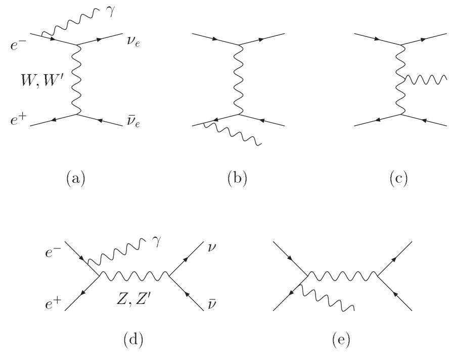
FIG. 1.: The Feynman diagrams contributing to the process $e^{+}e^{-}\rightarrow\nu\bar{\nu}\gamma$ in leading order.

FIG. 2.: The total cross sections $\sigma$, $\sigma_{L}$ and $\sigma_{R}$ versus $\sqrt{s}$ for $M_{W^{\prime}}=750$ GeV. For $\sigma_{L}$ and $\sigma_{R}$, 100% $e^{-}$ polarization is used. Results are given for the SM (solid line), LRM (dashed line), KK model (dotted line), UUM (dash-dotted line), SSM($W^{\prime}$) (thick dashed line) and SSM($W^{\prime}+Z^{\prime}$) (thick dash-dotted line).

FIG. 3.: (a) Left-handed differential cross section versus energy; (b) relative statistical significance of the deviation from the SM, for $\sqrt{s}=500$ GeV and $M_{W^{\prime}}=750$ GeV. 100% $e^{-}$ polarization is used. Lines as in Fig. 2.

FIG. 4.: (a) Right-handed differential cross section versus energy; (b) relative statistical significance of the deviation from the SM, for $\sqrt{s}=500$ GeV and $M_{W^{\prime}}=750$ GeV. 100% $e^{-}$ polarization is used. Lines as in Fig. 2.

FIG. 5.: (a) Left-handed differential cross section versus $\cos\theta_{\gamma}$; (b) relative statistical significance of the deviation from the SM, for $\sqrt{s}=500$ GeV and $M_{W^{\prime}}=750$ GeV. 100% $e^{-}$ polarization is used. Lines as in Fig. 2.

FIG. 6.: (a) Right-handed differential cross section versus $\cos\theta_{\gamma}$; (b) relative statistical significance of the deviation from the SM, for $\sqrt{s}=500$ GeV and $M_{W^{\prime}}=750$ GeV. 100% $e^{-}$ polarization is used. Lines as in Fig. 2.

FIG. 7.: LRM ($\rho=1$) unpolarized 95% C.L. $W^{\prime}$ mass limits versus $\kappa$, obtained for $\sqrt{s}=500$, 1000, 1500 and 2000 GeV using $d\sigma/dE_{\gamma}$ as the observable and an integrated luminosity of 50 fb^-1 for $\sqrt{s}=500$ GeV and 200 fb^-1 for the higher energies. Only statistical errors are used.

FIG. 8.: As Fig. 7, except (a) for 90% right-polarized electrons, (b) for 100% right-polarized electrons.

FIG. 9.: UUM unpolarized 95% C.L. $W^{\prime}$ mass limits versus $\sin\phi$, obtained for $\sqrt{s}=500$, 1000, 1500 and 2000 GeV using $d\sigma/dE_{\gamma}$ as the observable and an integrated luminosity of 50 fb^-1 for $\sqrt{s}=500$ GeV and 200 fb^-1 for the higher energies. Only statistical errors are used. The region to the right of the various curves is the region which may be excluded by experiment.

FIG. 10.: Constraints on the $Z^{\prime}\nu\bar{\nu}$ couplings $R_{\nu}(Z^{\prime})$ and $L_{\nu}(Z^{\prime})$ below the $Z^{\prime}$ peak using different observables. We take $\sqrt{s}=0.5$ TeV, $\ M_{Z^{\prime}}=1.5$ TeV and $L_{\rm int}=500$ fb^-1, except in the indicated case where it is $50$ fb^-1. The polarization of the electron beam is 90% and the positron beam is unpolarized, except in the indicated case where it is 60% polarized. Only statistical errors are included in this figure, except in the indicated case where a systematic error of 1% is included for $\sigma$. The assumed model is a $Z^{\prime}$ in the Sequential Standard Model [SSM ($Z^{\prime}$)], indicated by a star.

FIG. 11.: Constraints on $R_{\nu}(Z^{\prime})$ and $L_{\nu}(Z^{\prime})$ below the $Z^{\prime}$ peak using $\sigma$ and $A_{LR}$ combined as observables. The lines show the results for two different $Z^{\prime}$ masses. The dots indicate how the constraints relax if the error on the $Z^{\prime}e^{+}e^{-}$ coupling measurement is included as described in the text. We take $\sqrt{s}=0.5$ TeV, $L_{\rm int}=500$ fb^-1 and a systematic error of 2% (1%) for $\sigma$ ($A_{LR}$). The assumed model [SSM ($Z^{\prime}$)] is indicated by a star.

FIG. 12.: Constraints on the $W^{\prime}$ couplings using $\sigma$, $A_{LR}$ and using $\sigma$ and $A_{LR}$ combined as observables. We take $\sqrt{s}=0.5$ TeV, $L_{\rm int}=500$ fb^-1 and $M_{W^{\prime}}=1.5$ TeV. Only statistical errors are included in this figure. 90% electron and, where indicated, 60% positron polarization are used. The assumed model [SSM ($W^{\prime}$)] is indicated by a star.

FIG. 13.: Constraints on the $W^{\prime}$ couplings using $\sigma$ and $A_{LR}$ combined. 90% electron and 60% positron polarization are used. We take $\sqrt{s}=0.5$ TeV, $M_{W^{\prime}}=1.5$ TeV and $L_{\rm int}=500$ fb^-1, except in the indicated case where it is $50$ fb^-1. Only statistical errors are used, except in the indicated case where a systematic error of 2% (1%) is included for $\sigma$ ($A_{LR}$). The assumed model [SSM ($W^{\prime}$)] is indicated by a star.

FIG. 14.: Constraints on the $W^{\prime}$ couplings using $\sigma$ and $A_{LR}$ combined for different $W^{\prime}$ masses. We take 90% electron and 60% positron polarization, $\sqrt{s}=0.5$ TeV and $L_{\rm int}=500$ fb^-1. A systematic error of 2% (1%) is included for $\sigma$ ($A_{LR}$). The assumed model [SSM ($W^{\prime}$)] is indicated by a star.

FIG. 15.: Constraints on the $W^{\prime}$ couplings using $\sigma$ and $A_{LR}$ combined for different $W^{\prime}$ scenarios. We take 90% electron and 60% positron polarization, $\sqrt{s}=0.5$ TeV, $L_{\rm int}=500$ fb^-1 and $M_{W^{\prime}}=0.75$ TeV. A systematic error of 2% (1%) is included for $\sigma$ ($A_{LR}$). The assumed models are indicated by stars.

FIG. 16.: Constraints on the $W^{\prime}$ couplings using $\sigma$ and $A_{LR}$ combined in the LRM with $\rho=1$ and $\kappa=1$ for different $W^{\prime}$ masses and different fitting strategies; see text. We take 90% electron and 60% positron polarization, $\sqrt{s}=0.5$ TeV and $L_{\rm int}=500$ fb^-1. A systematic error of 2% (1%) is included for $\sigma$ ($A_{LR}$). The assumed model (LRM) is indicated by a star.

FIG. 17.: Constraints on the $W^{\prime}$ couplings using $\sigma$ and $A_{LR}$ combined in the UUM with $\sin\phi=0.6$ for different $W^{\prime}$ masses and different fitting strategies; see text. We take 90% electron and 60% positron polarization, $\sqrt{s}=0.5$ TeV and $L_{\rm int}=500$ fb^-1. Unless otherwise indicated, a systematic error of 2% (1%) is included for $\sigma$ ($A_{LR}$). The coupling of the assumed model (UUM) is indicated by a star.

TABLE I.: $W^{\prime}$ 95% C.L. discovery limits obtained in the SSM ($W^{\prime}$), SSM ($W^{\prime}+Z^{\prime}$), LRM ($\kappa=\rho=1$), UUM ($\sin\phi=0.6$), and the KK model using $d\sigma/dE_{\gamma}$ as the observable. Results are presented for $\sqrt{s}=500$, 1000, and 1500 GeV and for various luminosity and polarization scenarios, with and without a 2% systematic error included. For the LRM, the polarized scenario corresponds to a right-handed $e^{-}$ beam, while for all other models the beam is left-handed.

	Lum. (fb-1):	50	500	25	250	50	500	25	250
$\sqrt{s}$	Sys. Err.:	0%	0%	0%	0%	2%	2%	2%	2%
(GeV)	Model/% pol:	unp.	unp.	90%	90%	unp.	unp.	90%	90%
500	SSM($W^{\prime}$)	2.4	4.3	2.4	4.3	1.55	1.7	1.55	1.7
	SSM($W^{\prime}+Z^{\prime}$)	1.75	3.25	1.8	3.25	1.1	1.2	1.15	1.25
	LRM	0.75	1.15	0.85	1.25	0.6	0.6	0.75	1.0
	UUM	0.65	2.1	0.65	2.05	0.6	0.6	0.6	0.6
	KK	2.55	4.55	2.6	4.65	1.6	1.75	1.7	1.85
1000	Lum. (fb-1):	200	500	100	250	200	500	100	250
	SSM($W^{\prime}$)	4.2	5.3	4.2	5.25	2.15	2.2	2.1	2.2
	SSM($W^{\prime}+Z^{\prime}$)	3.15	4.0	3.2	4.1	1.1	1.1	1.15	1.45
	LRM	1.35	1.55	1.35	1.6	0.95	0.95	1.25	1.35
	UUM	1.25	2.45	1.25	2.35	1.1	1.1	1.1	1.1
	KK	4.55	5.75	4.6	5.85	2.15	2.2	2.25	2.3
1500	Lum. (fb-1):	200	500	100	250	200	500	100	250
	SSM($W^{\prime}$)	4.7	5.95	4.65	5.85	2.45	2.55	2.45	2.55
	SSM($W^{\prime}+Z^{\prime}$)	3.4	4.45	3.45	4.5	1.45	1.45	1.55	1.55
	LRM	1.65	1.9	1.7	1.9	1.3	1.3	1.55	1.65
	UUM	1.8	1.85	1.8	1.85	1.55	1.55	1.55	1.55
	KK	5.05	6.45	5.1	6.45	2.35	2.45	2.45	2.55

REFERENCES

- [1] For a recent review see M. Cvetic̆ and S. Godfrey; in Electroweak Symmetry Breaking and Beyond the Standard Model, eds. T. Barklow et al. (World Scientific, 1995), p. 383, hep-ph/9504216. See also Ref. [29].
- [2] S. Godfrey, Phys. Rev. D 51, 1402 (1995).
- [3] R.W. Robinett, Phys. Rev. D 26, 2388 (1982); R.W. Robinett and J.L. Rosner, ibid. D 25 3036 (1982); ibid. D 26, 2396 (1982); ibid. D 27, 679(E) 1983; P. Langacker, R.W. Robinett, and J.L. Rosner, Phys. Rev. D 30, 1470 (1984).
- [4] For a review and original references see R.N. Mohapatra, Unification and Supersymmetry (Springer, New York, 1986).
- [5] I. Antoniadis, Phys. Lett. B 246, 377 (1990); J. Lykken, Phys. Rev. D 54, 3693 (1996); E. Witten, Nucl. Phys. B471, 135 (1996); N. Arkani-Hamed, S. Dimopoulos, and G. Dvali, Phys. Lett. B 429, 263 (1998); I. Antoniadis, N. Arkani-Hamed, S. Dimopoulos, and G. Dvali, Phys. Lett. B 436, 257 (1998); N. Arkani-Hamed, S. Dimopoulos, and G. Dvali, Phys. Rev. D 59, 086004 (1999).
- [6] G. Barenboim, J. Bernabéu, J. Prades, and M. Raidal, Phys. Rev. D 55, 4213 (1997).
- [7] C. Caso et al., Particle Data Group, Eur. Phys. J. C3, 1 (1998).
- [8] T. Rizzo; in New Directions for High-Energy Physics: Proceedings of the 1996 DPF/DPB Summer Study on High-Energy Physics, Snowmass, Colorado, 1996, edited by D.G. Cassel, L. Trindle Gennari, and R.H. Siemann (Stanford Linear Accelerator Center, 1997), p. 900, hep-ph/9609248; p. 864, hep-ph/9612440.
- [9] J. Hewett; in New Directions for High-Energy Physics: Proceedings of the 1996 DPF/DPB Summer Study on High-Energy Physics, Snowmass, Colorado, 1996, edited by D.G. Cassel, L. Trindle Gennari, and R.H. Siemann (Stanford Linear Accelerator Center, 1997), p. 887, hep-ph/9704292.
- [10] H. Georgi, E.E. Jenkins, and E.H. Simmons, Phys. Rev. Lett. 62, 2789 (1989); ibid. 63, 1540(E) (1989); Nucl. Phys. B331, 541 (1990).
- [11] V. Barger and T.G. Rizzo, Phys. Rev. D 41, 946 (1990).
- [12] M. Masip and A. Pomeral, Phys. Rev. D 60, 096005 (1999); T.G. Rizzo and J.D. Wells, Report Nos. SLAC-PUB-8119, CERN-TH/99-139, hep-ph/9906234; G.F. Giudice, R. Rattazzi, and J.D. Wells, Nucl. Phys. B544, 3 (1999); T. Han, J. Lykken, and R.-J. Zhang, Phys. Rev. D 59, 105006 (1999).
- [13] M. Parida and A. Raychaudhuri, Phys. Rev. D 26, 2364 (1982).
- [14] D. Chang, R. Mohapatra, and M. Parida, Phys. Rev. D 30, 1052 (1984).
- [15] J.L. Hewett and T.G. Rizzo, Phys. Rev. D 47, 4981 (1993).
- [16] P. Langacker and S. Uma Sankar, Phys. Rev. D 40, 1569 (1989).
- [17] J. Chay, K.Y. Lee, and S.-H. Nam, Report No. SNUTP-98-101, hep-ph/9809298.
- [18] R. Kleiss and W.J. Stirling, Nucl. Phys. B262, 235 (1985).
- [19] F.A. Berends and W. Giele, Nucl. Phys. B294, 700 (1987).
- [20] J.A.M. Vermaseren, Symbolic Manipulation with FORM (CAN, Amsterdam, 1991).
- [21] F.A. Berends, G.J.H. Burgers, C. Mana, M. Martinez, and W.L. van Neerven, Nucl. Phys. B301, 583 (1988).
- [22] P.A. Baikov et al., Physical Results by means of CompHEP; in Proc. of X Workshop on High Energy Physics and Quantum Field Theory (QFTHEP-95), Moscow, 1996, edited by B. Levtchenko and V. Savrin, p. 101, hep-ph/9701412; E.E. Boos, M.N. Dubinin, V.A. Ilyin, A.E. Pukhov, and V.I. Savrin, hep-ph/9503280.
- [23] G. Montagna, M. Moretti, O. Nicrosini, and F. Piccinini, Nucl. Phys. B541, 31 (1999).
- [24] G. Montagna, O. Nicrosini, and F. Piccinini, Comput. Phys. Commun. 98, 206 (1996).
- [25] A. Denner, S. Dittmaier, M. Roth, and D. Wackeroth, Report No. BI-TP-99-10, hep-ph/9904472.
- [26] I.F. Ginzburg et al., Nucl. Instrum. Methods, 205, 47 (1983); ibid 219, 5 (1984); C. Akerlof, Report No. UM-HE-81-59 (1981; unpublished).
- [27] A. Czarnecki and W.J. Marciano, Int. J. Mod. Phys. A13, 2235 (1998).
- [28] A. Leike and S. Riemann, Z. Phys. C 75, 341 (1997).
- [29] A. Leike, Phys. Rept. 317, 143 (1999).
- [30] S. Godfrey, P. Kalyniak, B. Kamal, and A. Leike; in Proceedings of MRST’99: High Energy Physics at the Millennium, Ottawa, Canada, 1999, edited by P. Kalyniak, S. Godfrey, and B. Kamal (AIP, 1999), p. 1, hep-ph/9907571; S. Godfrey, P. Kalyniak, B. Kamal, and A. Leike; presented at The International Workshop on Physics and Detectors at the Linear Collider, Sitges, Spain, 1999, hep-ph/9909422. To appear in proceedings.