Introducing Dynamical Triangulations to the Type IIB Superstrings

Abstract

In order to consider non-perturbative effects of superstrings, we try to apply dynamical triangulations to the type IIB superstrings. The discretized action is constructed from the type IIB matrix model proposed as a constructive definition of superstring theory. The action has the local N=2 supersymmetry explicitly, and has no extra fermionic degrees of freedom. We evaluate the partition function for some simple configurations and discuss constraints required from the finiteness of partition functions.

1 Motivation

From recent developments, the universal superstring picture arose, namely the five types of superstrings and the M-theory are different representations of a single fundamental theory. It is expected to be a constructive definition of superstrings. The matrix model defined on the basis of the 10-dimensional super Yang-Mills theory is considered to be one of such constructive superstring theories [1, 2, 3]. There have been some attempts to introduce the dynamical triangulations in superstrings as a lattice regularization [4, 5]. In this study, we consider the type IIB superstring model derived as the large $N$ limit of the $N\times N$ matrix theory [6]. The advantage of the type IIB superstring is that the action has the local N=2 supersymmetry explicitly, and has no extra fermionic degrees of freedom.

2 Type IIB random superstrings

The action of the type IIB matrix model is expressed in the semi-classical (i.e. large matrix size) limit by

$$S\!\!=\!\!\int\!\!d^{2}\sigma\sqrt{g}\left[\frac{1}{4}\{X^{\mu},X^{\nu}\}^{2}\!\!-\frac{i}{2}\bar{\theta}\Gamma_{\mu}\{X^{\mu},\theta\}\right]\!\!,$$ (1)

where the Poisson brackets $\{\;,\;\}$ are defined by

$$\{X,Y\}\equiv\frac{1}{\sqrt{g}}\epsilon^{ab}\partial_{a}X\partial_{b}Y.$$ (2)

Here, $X^{\mu}$ are the $d$-dimensional space-time coordinates and $\theta$ are anti-commuting spinor coordinates. Also, $g$ is the absolute value of determinant of the world-sheet metric ($g_{ab}$), and $\epsilon^{ab}$ is the anti-symmetric tensor. $S$ has the local $N=2$ supersymmetry for $d=3,4,6$ and $10$ cases, and the $N=2$ super transformations are given by

$$\left\{\begin{array}[]{lcl}\delta^{(1)}X^{\mu}&=&i\bar{\epsilon}_{1}\Gamma^{\mu}\theta\\ \delta^{(1)}\theta&=&-\frac{1}{2}\{X^{\mu},X^{\nu}\}\Gamma_{\mu\nu}\epsilon_{1},\end{array}\right.$$ (5)

$$\left\{\begin{array}[]{lcl}\delta^{(2)}X^{\mu}&=&0\\ \delta^{(2)}\theta&=&\epsilon_{2},\end{array}\right.$$ (8)

where $\Gamma^{\mu\nu}$ is an antisymmetric tensor defined by $\Gamma^{\mu\nu}=\frac{1}{2}[\Gamma^{\mu},\Gamma^{\nu}]$.

In order to obtain the discretized action corresponding to $S$, we perform triangulations of the world-sheet by equilateral triangles. By summing over contributions from each triangle with three vertices $i$, $j$ and $k$, the discretized type IIB superstring action is given by

$$S\sim \frac{\triangle}{2}\!\!\sum_{\langle ijk\rangle}\left[\frac{1}{4}\{X^{\mu},X^{\nu}\}_{\langle ijk\rangle}^{2}\right.$$

$$\left.-\frac{i}{4}\bar{\theta}_{\langle ijk\rangle}\Gamma^{\mu}\{X_{\mu},\theta\}_{\langle ijk\rangle}\!\!-\!\!\frac{i}{4}\{\bar{\theta},X_{\mu}\}_{\langle ijk\rangle}\Gamma^{\mu}\theta_{\langle ijk\rangle}\!\right]$$

$$=\hskip 8.53581pt \frac{1}{4\triangle}\sum_{\langle ijk\rangle}\left[-\frac{1}{4}\{(X_{ij}^{2})^{2}+(X_{jk}^{2})^{2}+(X_{ki}^{2})^{2}\}\right.$$ (9)

$$\hskip 25.60747pt+\frac{1}{2}\{X_{ij}^{2}X_{jk}^{2}+X_{jk}^{2}X_{ki}^{2}+X_{ki}^{2}X_{ij}^{2}\}$$

$$\hskip 8.53581pt-\frac{\triangle}{3}\{\Omega_{ij}\!\!\cdot\!\!(X_{jk}\!\!-\!\!X_{ki})\!+\!\Omega_{jk}\!\!\cdot\!\!(X_{ki}\!\!-\!\!X_{ij})$$

$$\hskip 71.13188pt\left.\!+\Omega_{ki}\!\!\cdot\!\!(X_{ij}\!\!-\!\!X_{jk})\}\frac{}{}\right].$$

Here, $\theta_{\langle ijk\rangle}=\frac{1}{3}(\theta_{i}+\theta_{j}+\theta_{k})$ is the average strength of the fermionic field for the triangle $\langle ijk\rangle$, and we denote $X_{ij}^{\mu}\equiv X_{i}^{\mu}-X_{j}^{\mu}$ and $\Omega_{ij}^{\mu}\equiv\frac{i}{2}(\bar{\theta}_{i}\Gamma^{\mu}\theta_{j}-\bar{\theta}_{j}\Gamma^{\mu}\theta_{i})$. $X^{\mu}_{i}$ and $\theta_{i}$ are bosonic and fermionic fields on a vertex $i$, respectively, and $\triangle$ is twice the area of elementary triangle. The discretized Poisson brackets are defined by

$$\{A,B\}_{\langle ijk\rangle} \equiv \frac{1}{\triangle}f_{ijk}(A_{jk}B_{ki}-B_{jk}A_{ki}),$$ (10)

where

$$f_{ijk} = \left\{\begin{array}[]{cl}+1&(i,\;j,\;k)\;{\rm counterclockwise}\\ -1&(i,\;j,\;k)\;{\rm clockwise}.\end{array}\right.$$ (13)

$S$ is invariant under the following descretized super transformations;

$$\left\{\begin{array}[]{lcl}\delta^{(1)}X_{i}^{\mu}&=&i\bar{\epsilon}_{1}\Gamma^{\mu}\theta_{i}\\ \delta^{(1)}\theta_{\langle ijk\rangle}&=&-\frac{1}{2}\{X^{\mu},X^{\nu}\}_{\langle ijk\rangle}\Gamma_{\mu\nu}\epsilon_{1},\end{array}\right.$$ (16)

$$\left\{\begin{array}[]{lcl}\delta^{(2)}X_{i}^{\mu}&=&0\\ \delta^{(2)}\theta_{i}&=&\epsilon_{2}.\end{array}\right.$$ (19)

Since the discretized Poisson bracket is constant on each triangle, the variation of the fermionic field $\delta^{(1)}\theta_{\langle ijk\rangle}$ is defined on the triangle. Then we must examine the one-to-one correspondence between the variations of fermionic variables on triangles and on vertices for the local supersymmetric invariance. In order to check the correspondence, we count the number of independent relations among the $N_{2}=2(N_{0}-\chi)$ equations,

$$\delta^{(1)}\theta_{\langle ijk\rangle} = \frac{1}{3}\left(\delta^{(1)}\theta_{i}+\delta^{(1)}\theta_{j}+\delta^{(1)}\theta_{k}\right),$$ (20)

with the Euler characteristic $\chi$. According to the attempt for numerical solutions of eq. (20), we find that there dose not exist the one-to-one correspondence only for those configurations which have extra spatial symmetry. Since these configurations are expected to possess degeneracy, we should include extra measure factors to impose the one-to-one correspondence.

3 Partition functions and numerical results

Quantization is carried out using a standard path-integral method. The path integration over $\sqrt{g}$ is interpreted as the sum over dynamical triangulations. For the type IIB superstring, the discretized partition function with a fixed number of vertices is given by

$$Z(N_{0})\! = \!\sum_{{\cal T}}\!\!\!\frac{1}{\cal S(T)}\!\!\int\!\!\prod_{i=0}^{N_{0}-1}\!\!\!dX_{i}d\theta_{i}d\bar{\theta}_{i}e^{-S_{B}-S_{F}}$$ (21)

$$\hskip 56.9055pt\times\;\delta(X_{0})\delta(\bar{\theta}_{0})\delta(\theta_{0}),$$

where ${\cal S(T)}$ is a symmetry factor of triangulations (${\cal T}$) to take into account the degeneracy. It is noted that the modes associated with the translational invariance of the action for bosonic fields and the $\delta^{(2)}$ supersymmetry for fermionic fields is eliminated by imposing $X_{0}=0$ and $\theta_{0}=\bar{\theta}_{0}=0$. However, there exist special configurations which give the zero fermion determinant. They don’t have the one-to-one correspondence between triangles and vertices resulting fermionic zero modes. In order to obtain the non-zero fermion determinant, we include extra constraint to kill dependent fermionic fields as $\prod_{k}^{{\tiny N_{0}^{dep.}}}\delta(\bar{\theta}_{k})\delta(\theta_{k})$, where $N_{0}^{dep.}$ is the number of dependent relations.

We will evaluate the partition function of a tetrahedron ($N_{0}=4$) configuration as shown by solid lines in Fig. 1. Their integration measures are defined by

$$\begin{array}[]{ccl}dX_{1}&=&x^{d-1}dxd\Omega_{d-1},\\ dX_{2}&=&dyz^{d-2}dzd\Omega_{d-2},\\ dX_{3}&=&\prod_{i=1}^{d}dx_{i}.\end{array}$$ (25)

By integrating out the fermionic coordinates, the partition function is given by

$$Z(4)\!\! \propto \!\!\int_{0}^{\infty}\!\!x^{d-1}z^{d-2}dxdz\!\!\int_{-\infty}^{\infty}\!\!dy\prod_{i=1}^{d}dx_{i}e^{-S_{B}}$$ (26)

$$\times\left[(x_{3}^{2}+\cdots+x_{d}^{2})x^{2}z^{2}\right]^{\frac{k}{2}}$$

$$\propto \int_{0}^{\infty}dXX^{\frac{1}{2}(d+k-2)}e^{-\frac{4}{3}X^{2}}$$

$$\times\!\!\int_{0}^{\frac{\pi}{2}}\!\!\!\!d\theta(\cos\theta)^{\frac{1}{2}(d+k-4)}(\sin\theta)^{\frac{1}{2}(d+k-6)}\!\!,$$

where

$$S_{B} \cong x^{2}z^{2}+(zx_{1}-yx_{2})^{2}+x_{2}^{2}x^{2}$$ (27)

$$+\{(y-x)x_{2}-(x_{1}-x)z\}^{2}$$

$$+2\{x^{2}+y^{2}+z^{2}-xy\}(x_{3}^{2}+\cdots+x_{d}^{2}).$$

We have defined $X^{2}\equiv x^{2}z^{2}$, $\tan\theta\equiv\frac{2}{\sqrt{3}}\frac{z}{x}$, and $\Gamma^{\mu}$ are $k\times k$ matrices. The condition in which the partition function is finite is $d+k>4$. In the case of a tetrahedron, even the partition function of the bosonic string becomes finite, when $d>4$. However, the situation is not so simple for larger size configurations. We have found numerically that the partition function of the bosonic string exhibits a spike singularity for large $N_{0}$ in the case of $d=5$.

In the case of a configuration with an additional vertex as shown in Fig. 1, where links of three triangles added by the 5th vertex is shown in dotted lines, we can obtain two conditions as $k>0$ and $2d+k>6$. The condition $k>0$ implies that contributions from fermionic fields are necessary for the finiteness of the partition function.

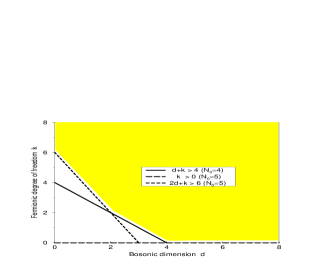
Figure 1: Solid lines denote a tetrahedron configuration, and adding dashed lines they denote a configuration with 5 vertices.

Figure 2: Constraint conditions from the analytic calculations for the partition functions of $N_{0}=4$ and 5 configurations. In the shadowed region, these three constraints are satisfied.

4 Summary

We have proposed the discretized type IIB superstring action, and have shown that it is invariant under the local N=2 super transformations. In the numerical study, the partition function of the bosonic strings exhibits a spike singularity for large configuration, and spike configurations dominate. From the study with $N_{0}=5$ configuration, we find that it is essential for the finiteness of the partition function to introduce fermionic fields. For further study, we need to find a powerful method to calculate the fermion determinants in a larger system.

References

• [1] T.ย Banks, W.ย Fischler, S.ย H.ย Shenker and L.ย Susskind, Phys.ย Rev.ย D55 (1997) 5112.
• [2] N.ย Ishibashi, H.ย Kawai, Y.ย Kitazawa and A.ย Tsuchiya, Nucl.ย Phys.ย B498 (1997) 467.
H.ย Aoki, S.ย Iso, H.ย Kawai, Y.ย Kitazawa and T.ย Tada, Prog.ย Theor.ย Phys.ย 99 (1998) 713.
• [3] H.ย Itoyama, A.ย Tokura, Prog.ย Theor.ย Phys.ย 97 (1997) 949; hep-th/9707002.
• [4] A.ย Mikoviฤ‡ and W.ย Siegel, Phys.ย Lett.ย B240 (1990), 363.
• [5] J.ย Ambรธrn and S.ย Varsted, Phys.ย Lett.ย B257 (1991), 305.
• [6] S.ย Oda, T.ย Yukawa, Prog.ย Theor.ย Phys.ย 102 (1999) 215; hep-th/9903261.