Pion decay constant for the Kogut-Susskind quark action in quenched lattice QCD

Abstract

We present a study for the pion decay constant $f_{\pi}$ in the quenched approximation to lattice QCD with the Kogut-Susskind (KS) quark action, with the emphasis given to the renormalization problems. Numerical simulations are carried out at the couplings $\beta=6.0$ and 6.2 on $32^{3}\times 64$ and $48^{3}\times 64$ lattices, respectively. The pion decay constant is evaluated for all KS flavors via gauge invariant and non-invariant axial vector currents with the renormalization constants calculated by both non-perturbative method and perturbation theory. We obtain $f_{\pi}=89(6)$ MeV in the continuum limit as the best value using the partially conserved axial vector current, which requires no renormalization. From a study for the other KS flavors we find that the results obtained with the non-perturbative renormalization constants are well convergent among the KS flavors in the continuum limit, confirming restoration of $\rm SU(4)_{A}$ flavor symmetry, while perturbative renormalization still leaves an apparent flavor breaking effect even in the continuum limit.

I Introduction

In recent large-scale simulations of lattice QCD, statistical errors of physical quantities have become quite small. Indeed, for some hadronic matrix elements the precision has been so high that we cannot ignore uncertainties coming from the renormalization factor of lattice operators. Thus it has become increasingly important to reduce uncertainties from this source.

Renormalization factors can be evaluated in perturbation theory. Pushing the calculation beyond the one-loop level is usually difficult, however, hence uncertainties arising from higher-order corrections remain. We expect this problem of higher-order uncertainties to profit fully from a non-perturbative treatment. A non-perturbative method for calculating renormalization factors was proposed[1], and has been applied to the quark mass[2], decay constants[3] and four-fermion operators[4], with the Wilson and the clover quark actions and to the quark mass with the Kogut-Susskind quark action[5].

An important point to check with non-perturbatively calculated renormalization factors is their reliability and the degree of improvement achieved in the final physical results. For this purpose the pion decay constant is perhaps the best choice because the reference experimental value is known to a high precision. A verification that non-perturbative determination works for simple quark bilinear operators is a first step to ensure validity of more general applications to four-quark or other operators.

In this work, the pion decay constant is examined with the Kogut-Susskind (KS) quark action via gauge invariant and non-invariant operators using all KS flavors. The KS action has the well-known feature that $\rm SU(4)_{A}$ flavor symmetry is broken down to $\rm U(1)_{A}$ subgroup at a finite lattice spacing. We orient our study mainly toward the following two points provided by this feature. First, due to the remaining $\rm U(1)_{A}$ symmetry, the renormalization constant for the corresponding axial vector current equals exactly unity, and hence the pion decay constant calculated in this channel receives no renormalization. This makes it possible to attain a high-precision calculation of the pion decay constant without uncertainties from renormalization. Second, we can calculate the pion decay constant using axial vector currents in the other KS flavor channels. Symmetry is broken in the decay constants at a finite lattice spacing, but restoration is expected in the continuum limit. Such restoration of full flavor symmetry has been previously examined for pion mass[6, 7]. Here we extend the study to the pion decay constant, the new feature being the necessity of renormalization constants. This can be used to investigate the reliability of non-perturbative methods for the calculation of renormalization factors, compared to perturbative treatments. We also compare the results obtained with gauge invariant operators to those with non-invariant ones.

The paper is organized as follows. In Sec. II we establish our notations and formalism. The method employed for our calculations is explained in Sec. III, followed by discussion of perturbative and non-perturbative renormalization factors in Sec. IV. We summarize the simulation details in Sec. V, and present the results on the chiral and continuum extrapolations in Secs. VI and VII. We close with a brief conclusion in Sec. VIII.

II Formulations

A Kogut-Susskind quark action

The Kogut-Susskind (KS) quark action is defined in terms of one-component fermion fields $\overline{\chi}(n)$ and $\chi(n)$ on a lattice whose site is labelled by $n_{\mu}=0,1,2,\ldots,L-1$,

$$S_{q}^{\rm KS}=a^{4}\sum_{n}\left[\sum_{\mu}\eta_{\mu}(n)\frac{1}{2a}\big{(}\overline{\chi}(n)U_{\mu}(n)\chi(n+\hat{\mu})\right.\>$$ (1)

$$-\overline{\chi}(n+\hat{\mu})U^{\dagger}_{\mu}(n)\chi(n)\big{)}+m_{q}\overline{\chi}(n)\chi(n)\left],\mbox{\rule{-10.0pt}{16.0pt}}\right.$$ (2)

where $m_{q}$ is the bare quark mass and $\eta_{\mu}=(-1)^{n_{1}+\cdots+n_{\mu-1}}$ is the KS sign factor. Color sums are assumed for simplicity. Dividing the lattice into $2^{4}$-hypercubes which are labelled by $x_{\mu}=0,2,4,\ldots,L-2$, and whose corners are specified by a four-vector $A$ with $A_{\mu}=0$ or 1, we introduce sixteen-component fields

$$\overline{\phi}_{A}(x)=\frac{1}{4}\overline{\chi}(x+A),\qquad\phi_{A}(x)=\frac{1}{4}\chi(x+A).$$ (3)

In terms of these hypercubic fields, the action (2) is rewritten as

$$S_{q}^{\rm KS}=(2a)^{4}\sum_{x,AB}\left[\sum_{\mu}\big{(}\overline{\phi}_{A}(x)(\gamma_{\mu}\otimes I)_{AB}\nabla_{\mu}U_{AB}\phi_{B}(x)\mbox{\rule{0.0pt}{16.0pt}}\right.\;\;\;\;\,$$ (4)

$$+a\overline{\phi}_{A}(x)(\gamma_{5}\otimes\xi_{\mu}\xi_{5})_{AB}\Delta_{\mu}U_{AB}\phi_{B}(x)\big{)}\;\;\;\>$$ (5)

$$\left.+m_{q}\overline{\phi}_{A}(x)(I\otimes I)_{AB}U_{AB}(x,x)\phi_{B}(x)\mbox{\rule{0.0pt}{16.0pt}}\right].$$ (6)

(7)

Here a hypercube matrix referring to the Dirac spinor $\gamma_{S}=\gamma_{1}^{S_{1}}\cdots\gamma_{4}^{S_{4}}$ and the KS flavor $\xi_{F}=\gamma_{1}^{*F_{1}}\cdots\gamma_{4}^{*F_{4}}$ is defined by

$$(\gamma_{S}\otimes\xi_{F})_{AB}=\frac{1}{4}{\rm Tr}(\gamma_{A}^{\dagger}\gamma_{S}\gamma_{B}\gamma_{F}^{\dagger})$$ (8)

and the lattice derivatives are given by

$$\nabla_{\mu}U_{AB}\phi_{B}(x) = \>\frac{1}{2a}\>\big{(}U_{AB}(x,y)\phi_{B}(y)|_{y=x+2\hat{\mu}}$$ (10)

$$\;\;\>\>\>\,-U_{AB}(x,y)\phi_{B}(y)|_{y=x-2\hat{\mu}}\big{)},$$

$$\Delta_{\mu}U_{AB}\phi_{B}(x) = \frac{1}{2a^{2}}\big{(}U_{AB}(x,y)\phi_{B}(y)|_{y=x+2\hat{\mu}}$$ (13)

$$\;\;\;\;\;+U_{AB}(x,y)\phi_{B}(y)|_{y=x-2\hat{\mu}}$$

$$\;\;\;\;\;-2U_{AB}(x,x)\phi_{B}(y)\big{)},$$

where $U_{AB}(x,y)$ is the average of ordered products of gauge link variables over the shortest paths from $x+A$ to $y+B$.

A gauge-invariant meson operator with zero spatial momentum is defined in this hypercubic notation by

$$O_{S}^{F}(x_{4})=\sum_{\vec{x}}\sum_{AB}\overline{\phi}_{A}(x)(\gamma_{S}\otimes\xi_{F})_{AB}U_{AB}(x,x)\phi_{B}(x).$$ (14)

For instance, $O_{S}=A_{\mu}$, $\pi$, and $\rho_{k}$ respectively for $\gamma_{S}=\gamma_{\mu}\gamma_{5}$, $\gamma_{5}$, and $\gamma_{k}$. Here we have $2^{4}\times 2^{4}=256$ operators, which are classified into irreducible representations[8] in terms of $d_{\mu}=S_{\mu}-F_{\mu}\,(\bmod{2})$.

The form of the action (7) shows that the flavor-mixing term $(\gamma_{5}\otimes\xi_{\mu}\xi_{5})$ breaks $\rm SU(4)_{A}$ flavor symmetry down to $\rm U(1)_{A}$ subgroup for the flavor channel $\xi_{5}$ at a finite lattice spacing. A lattice analog of the PCAC relation holds in the $\xi_{5}$ channel corresponding to $\rm U(1)_{A}$ symmetry:

$$\nabla_{\mu}A_{\mu}^{5}(x)=2m_{q}\pi^{5}(x),$$ (15)

where the superscript 5 refers to $\xi_{5}$. On the other hand, there appear additional terms in the PCAC relation for other channels, which vanish only in the continuum limit.

B Pion decay constant

The pion decay constant is defined in the continuum theory by

$$\sqrt{2}f_{\pi}m_{\pi}=\langle 0|\overline{u}\gamma_{4}\gamma_{5}d|\pi^{+}(\vec{p}=0)\rangle.$$ (16)

We adopt the normalization $f_{\pi}^{\rm(exp)}\simeq 93$ MeV. If we use the PCAC relation, this may be rewritten as

$$\sqrt{2}f_{\pi}m_{\pi}^{2}=(m_{u}+m_{d})\langle 0|\overline{u}\gamma_{5}d|\pi^{+}(\vec{p}=0)\rangle.$$ (17)

The lattice pion decay constant for the KS flavor $\xi_{F}$ is defined by

$$\sqrt{2}f_{\pi}^{F}m_{\pi}^{F}=\langle 0|A_{4}^{F}|\pi^{F}(\vec{p}=0)\rangle,$$ (18)

In the $\xi_{5}$ channel where the PCAC relation (15) holds, we may use an alternative formula corresponding to Eq. (17):

$$\sqrt{2}f_{\pi}^{(P)5}(m_{\pi}^{5})^{2}=2m_{q}\langle 0|\pi^{5}|\pi^{5}(\vec{p}=0)\rangle,$$ (19)

where we have added the superscript $(P)$ to distinguish explicitly the pion decay constant obtained with a pion operator from that with an axial vector current.

III Extraction of pion decay constant

We employ the wall source technique to enhance signals[9]. The meson operator for the wall source at the origin is defined by

$$O_{SW}^{F}(0)=\sum_{\vec{x},\vec{y}}\overline{\phi}_{A}(\vec{x},0)(\gamma_{S}\otimes\xi_{F})_{AB}\phi_{B}(\vec{y},0),$$ (20)

where we assume that gauge configurations are fixed to some gauge. The matrix elements appearing in the definition of the pion decay constant are extracted from the large-time behavior of the correlation function at zero spatial momentum:

$$\langle O_{S}^{F}(t)\pi_{W}^{F}(0)\rangle$$ (25)

$$\sim C_{O_{S}\pi_{W}}^{F}(\sigma_{t})^{t}[\exp(-m_{\pi}^{F}t)\pm\exp(-m_{\pi}^{F}(T-t))],$$

$$\hskip 95.0pt\left\{\begin{array}[]{l}+\mbox{ sign for }O_{S}=\pi,\pi_{W},\\ -\mbox{ sign for }O_{S}=A_{4},\end{array}\right.$$

where $m_{\pi}^{F}$ is pion mass common to the three cases. Here we extend the time slice of meson operator defined at $x_{4}=0,2,4,\ldots,T-2$ to have $t=0,1,2,\ldots,T-1$ extensions with the temporal lattice size $T$. Note that there is no mixing between $\sigma_{t}=\pm 1$ states in this case with time-extended meson operators. The amplitude $C_{O_{S}\pi_{W}}^{F}$ can be written up to an overall sign factor as

$$C_{O_{S}\pi_{W}}^{F}=\frac{\langle 0|O_{S}^{F}|\pi^{F}(\vec{p}=0)\rangle\langle\pi^{F}(\vec{p}=0)|\pi_{W}^{F}|0\rangle}{2m_{\pi}^{F}V_{s}},$$ (26)

with $V_{s}$ the spatial lattice volume. Using the amplitude of the correlation functions with the axial vector current $(O_{S}=A_{4})$ and the pion operator for the wall source $(O_{S}=\pi_{W})$, the pion decay constant is calculated as

$$f_{\pi}^{F}=\frac{\sqrt{V_{s}}}{\sqrt{m_{\pi}^{F}}}\frac{C_{A_{4}\pi_{W}}^{F}}{\sqrt{C_{\pi_{W}\pi_{W}}^{F}}},$$ (27)

where the pion mass obtained by the correlation function with the pion operator ($O_{S}=\pi$) is used in this work. For comparison, the gauge non-invariant axial vector current and pion operator to obtain the amplitude and pion mass, respectively,

$${A_{4}^{\prime}}\mbox{}^{F}(x_{4}) = \sum_{\vec{x}}\sum_{AB}\overline{\phi}_{A}(x)(\gamma_{4}\gamma_{5}\otimes\xi_{F})_{AB}\phi_{B}(x),$$ (28)

$${\pi^{\prime}}\mbox{}^{F}(x_{4}) = \sum_{\vec{x}}\sum_{AB}\overline{\phi}_{A}(x)(\gamma_{5}\otimes\xi_{F})_{AB}\phi_{B}(x),$$ (29)

is also examined. Alternatively, an extraction of the decay constant from the pion operator $(O_{S}^{F}=\pi^{5})$ requires the combination given by

$$f_{\pi}^{(P)5}=\frac{\sqrt{2m_{q}V_{s}}}{\sqrt{(m_{\pi}^{5})^{3}}}\frac{C_{\pi\pi_{W}}^{5}}{\sqrt{C_{\pi_{W}\pi_{W}}^{5}}}.$$ (30)

IV Renormalization

A General considerations

Renormalization is necessary to extract the physical pion decay constant from the lattice calculations. This procedure is made for each flavor in the case of the KS action. It is expected that the renormalization eliminates the KS flavor dependence in a way that the decay constant calculated for various KS flavors takes a unique value in the continuum limit.

Let us define a multiplicative renormalization constant $Z_{A}^{F}$ for the lattice axial vector current $A_{\mu}^{F}\big{|}_{\rm lat}$ through

$$A_{\mu}^{F}\left|{}_{\rm phys}=Z_{A}^{F}A_{\mu}^{F}\right|_{\rm lat}.$$ (31)

According to the definition (18) the pion decay constant calculated with the axial vector current is renormalized as

$$f_{\pi}^{F}\left|{}_{\rm phys}=Z_{A}^{F}f_{\pi}^{F}\right|_{\rm lat}.$$ (32)

As a special case, we have

$$Z_{A}^{5}=1$$ (33)

in the $\xi_{5}$ channel due to the lattice PCAC relation (15). Thus the pion decay constant can be calculated with out any uncertainties of renormalization in this channel, while the other channels can be used to check the reliability of renormalization constants by examining the expected convergence of the renormalized pion decay constants to a single value in the continuum limit.

The decay constant defined with the pion operator (19) is renormalized as

$$f_{\pi}^{(P)5}\big{|}_{\rm phys}=(Z_{P}^{5}/Z_{m})f_{\pi}^{(P)5}\big{|}_{\rm lat},$$ (34)

where $Z_{m}$ is the renormalization constant for quark mass. Using the identities $Z_{m}=1/Z_{S}^{I}$ and $Z_{S}^{I}=Z_{P}^{5}$, where the superscript $I$ refers to the KS flavor for a unit matrix, we find that this relation is identical to

$$f_{\pi}^{(P)5}\big{|}_{\rm phys}=f_{\pi}^{(P)5}\big{|}_{\rm lat},$$ (35)

which is equivalent to Eq. (33).

B Perturbative and non-perturbative renormalization factors for axial vector currents

We employ two sets of the renormalization factor $Z_{A}^{F}$ for the KS axial vector current. One of them is perturbatively calculated at one-loop order[10]. We apply tadpole improvement to the axial vector current operator using the fourth root of plaquette as the tadpole factor, and evaluate the renormalization constants with the tadpole-improved $\overline{\rm MS}$ coupling at $q^{*}=1/a$. The other is non-perturbatively evaluated with the regularization independent (RI) scheme of Ref. [1], which was developed for the Wilson and clover actions. In the RI scheme, the renormalization factor is obtained from the amputated Green function in momentum space

$$\Gamma_{O_{S}}^{F}(p)=S(p)^{-1}\langle 0|\phi(p)O_{S}^{F}\overline{\phi}(p)|0\rangle S(p)^{-1},$$ (36)

where the quark two-point function is defined by $S(p)=\langle 0|\phi(p)\overline{\phi}(p)|0\rangle$, and the momentum of the hypercubic field $\phi(p)$ takes values of the form $p_{\mu}=2\pi n_{\mu}/(aL)$ with $-L/4\leq n_{\mu}\leq L/4-1$. The renormalization condition imposed upon $\Gamma_{O_{S}}^{F}(p)$ is given by

$$Z_{O_{S}}^{{\rm(RI)}F}(p)Z_{\phi}(p)={\rm Tr}[({\cal P}_{O_{S}}^{F})^{\dagger}\Gamma_{O_{S}}^{F}(p)],$$ (37)

where $\left({\cal P}_{O_{S}}^{F}\right)^{\dagger}=\big{(}\gamma_{S}^{\dagger}\otimes\xi_{F}^{\dagger}\big{)}$ is the projector onto the tree-level amputated Green function. The wave function renormalization constant $Z_{\phi}$ is calculated by imposing the condition $Z_{V}^{I}(p)=1$ for the conserved vector current for $(\gamma_{\mu}\otimes I)$. The relation between the overall renormalization constant $Z_{A}^{F}$ appearing in Eq. (31) and $Z_{A}^{{\rm(RI)}F}$ is simply

$$Z_{A}^{F}=1/Z_{A}^{{\rm(RI)}F},$$ (38)

because the continuum axial vector current is not renormalized.

The calculations for the non-perturbative renormalization constants were carried out in quenched QCD in our previous publication[5]. The results for the scalar and pseudoscalar operators have been used in our analysis of light quark masses for the KS quark action in quenched QCD[5]. Here we use them for the axial vector renormalization factors.

The calculational parameters are summarized in Table I. We evaluate the Green function (36) for 15 momenta in the range $0.038533\leq(pa)^{2}\leq 1.9277$ using quark propagators evaluated with a source in a momentum eigenstate. In Fig. 1 we present the renormalization constant for both vector and axial vector currents, respectively denoted by $Z_{V}^{{\rm(RI)}F}(p)$ and $Z_{A}^{{\rm(RI)}F}(p)$, in the chiral limit.

A practically important issue with the non-perturbative method employed here is the choice of the momentum at which the renormalization factors are evaluated. In general the momentum should satisfy $\Lambda_{\rm QCD}\ll p\ll O(a^{-1})$ in order to keep under control the non-perturbative hadronization effects and the discretization error on the lattice. Since these effects appear as $p$-dependences of renormalization factors, we should avoid the range where a momentum dependence is visible. Another point to consider is the relation $Z_{V}^{{\rm(RI)}F5}(p)=Z_{A}^{{\rm(RI)}F}(p)$ with the superscript $F5$ referring $\xi_{F}\xi_{5}$, which we would expect to hold for all momenta $p$ in the chiral limit due to $\rm U(1)_{A}$ chiral symmetry of the KS quark action.

For $\beta=6.2$ Fig. 1 shows that these two requirements are satisfied for $p^{2}>5$ GeV², which corresponds to $(pa)^{2}>0.5$. In order to satisfy $p\ll O(a^{-1})$, we take $(pa)^{2}=1.0024$ ($p^{2}=7.0392$ GeV² in physical units) to calculate the renormalization factors used for the pion decay constant. The same value of lattice momentum $(pa)^{2}=1.0024$ is chosen for $\beta=6.0$, which corresponds to $p^{2}=3.5428$ GeV². The numerical values of the renormalization factors are summarized in Table II.

V Details of simulation

A Simulation parameters

We carry out our calculations in quenched QCD using the standard plaquette action for gluons. As we summarize in Table III, numerical simulations are carried out at $\beta\equiv 6/g^{2}=6.0$ and 6.2 on $32^{3}\times 64$ and $48^{3}\times 64$ lattices, respectively. Gauge configurations are generated with the five-hit pseudo-heatbath algorithm, and hadron correlation functions are calculated on 100(60) configurations separated by 2000 sweeps at $\beta=6.0$(6.2).

Gauge configurations are fixed to the Landau gauge through maximization of

$$F_{L}=\sum_{n,\mu}{\rm tr}(U_{\mu}(n)+U^{\dagger}_{\mu}(n)).$$ (39)

This is realized by iterating the steepest descent method for the first 2000 steps and the over-relaxation method for the subsequent 3000 steps until the condition

$$\Delta=\frac{1}{6V}\sum_{n}{\rm tr}(G_{L}^{\dagger}(n)G_{L}(n))<10^{-14}$$ (40)

is satisfied, where $V$ is the lattice volume and

$$G_{L}=\sum_{\mu}\frac{1}{2}(U_{\mu}(n)-U_{\mu}(n-\hat{\mu})-\mbox{h.c.}-\mbox{trace}).$$ (41)

We take three values for quark mass, $m_{q}a=0.030$, 0.020, 0.010 at $\beta=6.0$ and 0.023, 0.015, 0.008 at $\beta=6.2$. Quark propagators are evaluated for 16 types of wall sources, each corresponding to a corner of a hypercube, defined by

$$\sum_{y,B}D_{AB}(x,y)\sum_{\vec{z}}G_{BC}(y,z)=\sum_{\vec{z}}\delta_{xz}\delta_{AC},$$ (42)

where $D_{AB}(x,y)$ is the quark matrix for the KS action. We solve the equation independently for each $C$ by the conjugate gradient method with the stopping condition

$$||\mbox{remnant vector}||^{2}<10^{-5}.$$ (43)

The 16 quark propagators are combined to construct the 16 meson correlation functions in the KS flavor basis specified by the hypercube matrix $\xi_{F}$. Averages are taken of the meson correlation functions over $2^{3}$ ways of choosing the spatial origin of hypercubes on the lattice. We also average them over all states belonging to the same irreducible representation[8].

B Fitting procedure

In fitting the meson correlation function $C(t)$ to the asymptotic form $C^{\rm fit}(t)$ for an extraction of the mass and amplitude, we symmetrize the correlator at $t$ and $T-t$, and carry out a standard correlated fit minimizing

$$\chi^{2}=\sum_{t,t^{\prime}}\Delta C(t)\Sigma^{-1}(t,t^{\prime})\Delta C(t^{\prime}),$$ (44)

where

$$\Sigma(t,t^{\prime})=\langle C(t)C(t^{\prime})\rangle-\langle C(t)\rangle\langle C(t^{\prime})\rangle$$ (45)

is the covariance matrix of the correlator and $\Delta C(t)=C(t)-C^{\rm fit}(t)$. The fitting range $t=t_{\rm min},\ldots,t_{\rm max}$ is chosen by fixing $t_{\rm max}=T/2$ and varying $t_{\rm min}$ so that $\chi^{2}/N_{\rm DF}$ takes a value near unity, where $N_{\rm DF}$ is the degree of freedom of the fit. Finally, errors in this work are estimated by the single elimination jackknife procedure.

C Wall-to-wall amplitude

We check the validity of the asymptotic form of the mesonic correlation function (25) which is based on the assumption of a single pole dominance by an inspection of the effective mass. Typical results for the effective mass extracted from the correlators $\langle\pi^{F}(t)\pi_{W}^{F}(0)\rangle$ and $\langle A_{4}^{F}(t)\pi_{W}^{F}(0)\rangle$ are compared in Fig. 2. We observe a wide plateau and an expected agreement of the effective masses from the two correlation functions. We then find no problem in fitting these correlation functions by a single pole.

The situation is different for the wall-to-wall correlation function $\langle\pi_{W}^{F}(t)\pi_{W}^{F}(0)\rangle$, particularly at $\beta=6.2$. As we show in Fig. 3, the effective mass for $\langle\pi_{W}^{F}(t)\pi_{W}^{F}(0)\rangle$ does not reach a plateau at $\beta=6.2$ even at $t\sim T/2$, and agreement with the effective mass of $\langle\pi^{F}(t)\pi_{W}^{F}(0)\rangle$ is not seen. This behavior is most likely caused by a lack of sufficient temporal size of the lattice, and poses a practical problem of how one extracts the wall-to-wall amplitude $C_{\pi_{W}\pi_{W}}^{F}$ which is needed in Eq. (27) to calculate the pion decay constant.

To solve this problem, we perform a double pole fit for $\langle\pi_{W}^{F}(t)\pi_{W}^{F}(0)\rangle$ given by

$$\langle\pi_{W}^{F}(t)\pi_{W}^{F}(0)\rangle$$ (48)

$$\sim C_{\pi_{W}\pi_{W}}^{F}(\sigma_{t})^{t}[\exp(-m_{\pi}^{F}\,t)+\exp(-m_{\pi}^{F}\,(T-t))]$$

$$\;+\;C_{q\overline{q}}^{F}\>\,[\exp(-m_{q\overline{q}}^{F}t)+\exp(-m_{q\overline{q}}^{F}(T-t))].$$

Ideally one likes to make a fit with four parameters $C_{\pi_{W}\pi_{W}}^{F}$, $m_{\pi}^{F}$, $C_{q\overline{q}}^{F}$, and $m_{q\overline{q}}^{F}$. This fit, however, is quite unstable because the fitting function consists of a sum of two exponentials with not much different masses $m_{\pi}^{F}$ and $m_{q\overline{q}}^{F}$. Therefore, we fix the pion mass parameter $m_{\pi}^{F}$ to that obtained from $\langle\pi^{F}(t)\pi_{W}^{F}(0)\rangle$.

As we now can no longer compare the effective pion mass for $\langle\pi_{W}^{F}(t)\pi_{W}^{F}(0)\rangle$ to that for $\langle\pi^{F}(t)\pi^{F}(0)\rangle$, we present a typical comparison of the amplitudes, extracted with the fitting range from $t$ to $T/2$ with the single and double pole fits, in Fig. 4. We also compare $\chi^{2}/N_{\rm DF}$ for the two fits in Fig. 5. From these figures, we consider that the double pole fit provides a good determination of the amplitude $C_{\pi_{W}\pi_{W}}^{F}$ of the pion to the wall operator with a wide plateau of the amplitude and a reasonable value of $\chi^{2}/N_{\rm DF}\sim O(1)$.

A possible interpretation for the dominant source of contamination to the wall-to-wall correlation function is an unbound quark-antiquark pair. Such a state can contribute since gauge configurations are fixed to the Landau gauge. In Fig. 6 we plot the value of the second pole mass $m_{q\overline{q}}$ as a function of quark mass. The fact that the results depend little on the KS flavor of the meson operator is consistent with this interpretation. In the chiral limit one obtains $m_{q\overline{q}}\sim 2\times 440$ MeV, which is a reasonable value for a constituent quark mass.

Finally, we summarize the fitting ranges $t_{\rm min}$ common for all flavors and $\chi^{2}/N_{\rm DF}$ for our global fits in Table IV. Here, we have used the alternative fitting range of the wall-to-wall correlation function to improve the fitting quality for $\xi_{F}=\xi_{4}$, because the common fitting range does not give a satisfactory result[11] caused by worse fitting.

VI Chiral behavior

A Pion masses

We show values of $(m_{\pi}^{F}a)^{2}$ as a function of $m_{q}a$ in Fig. 7. Pions for the 16 KS flavors are classified into 8 irreducible representations. These consist of four 1-dimensional representations given by $\xi_{5}$, $\xi_{4}\xi_{5}$, $\xi_{4}$, $I$ and four 3-dimensional representations given by $\xi_{k}\xi_{5}$, $\xi_{k}\xi_{4}$, $\xi_{k}\xi_{\ell}$, $\xi_{k}$ $(k,\ell=1,2,3;k<\ell)$. We observe very clearly in Fig. 7 that these irreducible representations form a degeneracy pattern specified by

$$\xi_{5},(\xi_{k}\xi_{5},\xi_{4}\xi_{5}),(\xi_{k}\xi_{4},\xi_{k}\xi_{\ell}),(\xi_{4},\xi_{k}),I.$$ (49)

This pattern was observed long time ago in Ref. [9]. A theoretical explanation based on the effective chiral Lagrangian analysis for KS quark action was provided recently in Ref. [12].

Another notable feature in Fig. 7 is a linear behavior of pion masses as a function of quark mass from the correlation function with the gauge invariant pion operator. With a linear extrapolation we observe a non-vanishing value at $m_{q}a=0$ in channels other than $\xi_{5}$ for which $\rm U(1)_{A}$ symmetry holds. The gauge non-invariant case, not presented in the figure but in Table V for the numerical values, also shows almost the same result as in Fig. 7.

The chiral behavior of $\rho$ meson mass for various KS flavors is shown in Fig. 8. We find the difference of masses among various flavor channels to be small, less than 1% even in the chiral limit obtained by a linear extrapolation. We therefore choose the $\rho$ meson mass in the flavor channel $(\gamma_{k}\otimes\xi_{k})$, for which the $\rho$ meson operator is local, to set the scale using the experimental value $m_{\rho}=770$ MeV. We then find that $a^{-1}=1.92(2)$ GeV for $\beta=6.0$ and $a^{-1}=2.70(5)$ GeV for $\beta=6.2$.

B Pion decay constant

In Fig. 9 we illustrate the chiral behavior of the bare pion decay constants calculated with Eq. (27). As with the case for pion masses, we use a linear extrapolation toward the chiral limit.

The pion decay constants obtained for eight irreducible representations again form a degeneracy pattern, which, however, is different from that for pion masses. This is due to the fact that the pattern for the decay constant reflects the distance of the axial vector current operator rather than that of the pion operator: the two operators differ because of the the Dirac factor, $\gamma_{4}\gamma_{5}$ for the axial vector current and $\gamma_{5}$ for the pion. We also observe that the KS flavor dependence of the decay constant is much larger for the gauge invariant operators than that for the non-invariant ones. In contrast to the case of mass, for which no renormalization is required and lattice symmetry group controls, the pattern for pion decay constants mainly comes from the insertion of gauge link variables, which is roughly written as relation between the continuum and lattice axial vector currents:

$$A_{\mu}\big{|}_{\rm cont}\sim\left(\frac{1}{3}\langle{\rm Tr}\,U_{\Box}\rangle\right)^{\!\mbox{$\frac{d-1}{4}$}}A_{\mu}^{F}\big{|}_{\rm lat}.$$ (50)

Here $d$ is the distance of the axial vector current operator for the gauge invariant case, while the non-invariant operator corresponds to $d=0$.

We show the decay constants after renormalization in Figs. 10 and 11. With the use of perturbative renormalization constants (Fig. 10), the discrepancy among different KS flavor channels becomes smaller toward the continuum. The reduction of the discrepancy, however, is significantly more dramatic with the use of non-perturbative renormalization constants as shown in Fig. 11. In particular, the large difference among bare results obtained with gauge invariant operators almost disappears.

The numerical values for pion decay constants are collected in Tables VI–VIII. In contrast to the case of pion mass, there is no flavor channel to give the same results for the gauge invariant and non-invariant case, because the simultaneous local channel does not exist for the axial vector current and the pion operator both appearing in the calculation of the pion decay constant.

VII Continuum extrapolation

In Fig. 12, we present $a$-dependence of $(m_{\pi}^{F})^{2}$ quadratically extrapolated to $m_{q}a=0$, according to $O(a^{2})$ scale violation expected for the KS quark action. We observe clear evidence that the non-zero values of $(m_{\pi}^{F})^{2}$ for the non-Nambu-Goldstone channels vanish as $a^{2}$ toward the continuum limit, supporting the restoration of full flavor symmetry of the KS action.

The continuum extrapolation of the pion decay constant, renormalized perturbatively or non-perturbatively, is shown in Fig. 13 as a function of $a^{2}$. In this figure with an enlarged vertical scale as compared to Figs. 10 and 11, we observe a general trend that the difference of values among various KS flavors becomes smaller toward the continuum limit. In particular, for non-perturbatively renormalized decay constants the central values in the continuum limit agree within a 2% accuracy, which is well below the statistical errors of 5–10%. On the other hand, the convergence is worse for the perturbatively renormalized decay constants. The spread in the continuum limit is 3–4%, which is roughly the magnitude of uncertainty one expects from higher-order corrections in the renormalization factors. We consider that these results provide evidence for both restoration of $\rm SU(4)_{A}$ flavor symmetry of the KS action in the continuum limit and the effectiveness of the non-perturbatively evaluated renormalization constants.

The values of pion mass squared for various KS flavors are listed in Table IX, and those for pion decay constants are collected in Tables X and XI. As our best value for the decay constant, we take $f_{\pi}=89(6)$ MeV obtained with the gauge invariant axial vector current in the $\xi_{5}$ channel which requires no renormalization. This value is compared with the experiment 92.4(3) MeV[13]. Possible quenching errors are not visible within the statistical error of 6 MeV.

Let us recall that the decay constant in the $\xi_{5}$ channel can also be calculated from the pion operator using Eqs. (30) and (35). Results are added in the bottom lines of Table X (and XI for convenience of readers), which show reasonable agreement with those from the axial vector current in the $\xi_{5}$ channel, as expected.

VIII Conclusion

In this article we have presented an analysis of the pion decay constant in quenched QCD using the Kogut-Susskind quark action. Our best estimate for the decay constant in the continuum limit is 89(6) MeV, which is obtained with the gauge invariant axial vector current which respects $\rm U(1)_{A}$ symmetry.

We have carried out a detailed comparison of perturbative and non-perturbative axial vector renormalization treatments. We conclude that the non-perturbative renormalization factors efficiently eliminate the flavor breaking effect in the decay constant in the continuum limit, while an apparent flavor-dependent difference still remains with the perturbative factors.

FIG. 1.: Non-perturbative renormalization constants for vector $Z_{V}^{F}(p)$ and axial vector currents $Z_{A}^{F}(p)$ examined with gauge invariant current for (a) $\beta=6.0$ and (b) $\beta=6.2$, and by gauge non-invariant current for (c) $\beta=6.0$ and (d) $\beta=6.2$.

FIG. 2.: Typical comparison of the effective mass of axial vector current (open symbols) and pion (filled symbols) correlation functions with its global mass (horizontal lines) for $\xi_{F}=\xi_{5}$ at (a) $\beta=6.0$ and (b) $\beta=6.2$. Circles, squares and diamonds refer to the quark masses in descending order at each coupling respectively. Note that result does not depend on gauge invariance of the operator in the case using local operator like this case.

FIG. 3.: Typical comparison of the effective masses of the wall-to-wall correlation function (open symbols) and that for pion correlation function (filled symbols) with its global mass (horizontal lines) for $\xi_{F}=\xi_{5}$ at (a) $\beta=6.0$ and (b) $\beta=6.2$.

FIG. 4.: Typical comparison of of the amplitude of wall-to-wall pion correlation function for $\xi_{F}=\xi_{5}$ at $\beta=6.2$ obtained by (a) the single pole fit and (b) the double pole fit.

FIG. 5.: Typical comparison of $\chi^{2}/N_{\rm DF}$ for (a) the single pole fitting and (b) the double pole fitting of wall-to-wall pion correlation function for $\xi_{F}=\xi_{5}$ at $\beta=6.2$.

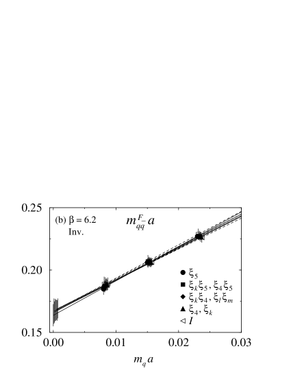
FIG. 6.: Chiral behavior of the alternative pole masses appearing in the wall-to-wall correlation function at (a) $\beta=6.0$ and (b) $\beta=6.2$. Shape of symbols refer to the distance of the operator. Some symbols (square, diamond and up-triangle) denotes two flavors; the former one refers time-local operators (filled symbols) including flavor $\xi_{5}$, and the latter one refers time-separated operators (open symbols).

FIG. 7.: Chiral behavior of pion masses obtained with the gauge invariant pion operators at (a) $\beta=6.0$ and (b) $\beta=6.2$. Shape of symbols refer to the distance of the operator. Some symbols denotes two flavors; the former one refers time-local operators (filled symbols) including flavor $\xi_{5}$, and the latter one refers time-separated operators (open symbols). For gauge non-invariant result, see Table V.

FIG. 8.: Chiral behavior of gauge-invariant $\rho$ meson masses at (a) $\beta=6.0$ and (b) $\beta=6.2$. Symbols refer to the distance of the operator, Some symbols denotes four flavors; the first two flavors refer time-local operators (filled symbols), and the last two flavors refer time-separated operators (open symbols).

FIG. 9.: Chiral behavior of the bare pion decay constants obtained by gauge invariant axial vector current for (a) $\beta=6.0$ and (b) $\beta=6.2$, and by gauge non-invariant current for (c) $\beta=6.0$ and (d) $\beta=6.2$. Omitted legends in the top two figures are same as that in the bottom figures. Shape of symbols refer to the distance of the operator. Some symbols denotes two flavors; the former one refers time-separated operators (filled symbols) including flavor $\xi_{5}$, and the latter one refers time-local operators (open symbols).

FIG. 10.: Pion decay constant renormalized by one-loop perturbative renormalization factor $Z_{A}^{(P)F}f_{\pi}^{F}$. Figures (a)–(d) correspond to those in Fig. 9.

FIG. 11.: Pion decay constant renormalized by non-perturbative renormalization factor $Z_{A}^{(N)F}f_{\pi}^{F}$. Figures (a)–(d) correspond to those in Fig. 9.

FIG. 12.: Continuum limit of pion mass squared. Symbols are same as those in Fig. 7.

FIG. 13.: Continuum limit of renormalized pion decay constants. Results obtained with perturbative renormalization factors for (a) gauge-invariant and (b) non-invariant operator, and those with non-perturbative factors for (c) gauge-invariant and (d) non-invariant operator are shown. Symbols are same as those in Figs. 9–11.

TABLE I.: Calculation parameters for evaluation of non-perturbative renormalization constants.

$\beta$	$L^{3}\times T$	$m_{q}a$	$a^{-1}$(GeV)	#conf.
6.0	$32^{3}\times 32$	0.010, 0.020, 0.030	1.88(4)	30
6.2	$32^{3}\times 32$	0.008, 0.015, 0.023	2.65(9)	30

TABLE II.: Renormalization constants $Z_{A}^{F}$ used for renormalizing pion decay constants.

(a) $\beta=6.0$
	Perturbative		Non-perturbative
Operator	Gauge inv.	Non-inv.	Gauge inv.	Non-inv.
$(\gamma_{4}\gamma_{5}\otimes\xi_{5})$	1	0.8917	1	0.85019(7)
$(\gamma_{4}\gamma_{5}\otimes\xi_{k}\xi_{5})$	1.1436	0.8547	1.2008(1)	0.8527(1)
$(\gamma_{4}\gamma_{5}\otimes\xi_{k}\xi_{4})$	1.3749	0.8556	1.4799(2)	0.8656(1)
$(\gamma_{4}\gamma_{5}\otimes\xi_{4})$	1.4950	0.8569	1.8242(3)	0.8736(2)
$(\gamma_{4}\gamma_{5}\otimes\xi_{4}\xi_{5})$	0.7908	0.7908	0.7976(2)	0.7976(2)
$(\gamma_{4}\gamma_{5}\otimes\xi_{\ell}\xi_{m})$	0.9294	0.8277	0.9860(1)	0.8508(1)
$(\gamma_{4}\gamma_{5}\otimes\xi_{k})$	1.1440	0.8550	1.2294(3)	0.8767(2)
$(\gamma_{4}\gamma_{5}\otimes I)$	1.3837	0.8605	1.5145(5)	0.8835(2)

(b) $\beta=6.2$
	Perturbative		Non-perturbative
Operator	Gauge inv.	Non-inv.	Gauge inv.	Non-inv.
$(\gamma_{4}\gamma_{5}\otimes\xi_{5})$	1	0.8917	1	0.86430(7)
$(\gamma_{4}\gamma_{5}\otimes\xi_{k}\xi_{5})$	1.1338	0.8643	1.1783(1)	0.86363(7)
$(\gamma_{4}\gamma_{5}\otimes\xi_{k}\xi_{4})$	1.3434	0.8651	1.4221(2)	0.8739(2)
$(\gamma_{4}\gamma_{5}\otimes\xi_{4})$	1.4567	0.8663	1.7164(3)	0.8803(2)
$(\gamma_{4}\gamma_{5}\otimes\xi_{4}\xi_{5})$	0.8065	0.8065	0.8136(1)	0.8136(1)
$(\gamma_{4}\gamma_{5}\otimes\xi_{\ell}\xi_{m})$	0.9369	0.8401	0.9838(1)	0.8600(1)
$(\gamma_{4}\gamma_{5}\otimes\xi_{k})$	1.1342	0.8646	1.1999(1)	0.8825(2)
$(\gamma_{4}\gamma_{5}\otimes I)$	1.3508	0.8696	1.4472(4)	0.8882(2)

TABLE III.: Calculation parameters of our simulation.

$\beta$	$L^{3}\times T$	$m_{q}a$	$a^{-1}$(GeV)	#conf.
6.0	$32^{3}\times 64$	0.010, 0.020, 0.030	1.92(2)	100
6.2	$48^{3}\times 64$	0.008, 0.015, 0.023	2.70(5)	60

TABLE IV.: Minimum time slice $t_{\rm min}$ common for all flavors except for $\xi_{F}=\xi_{4}$ in the parenthesis (See text for reason), and $\chi^{2}/N_{\rm DF}$ of global fits for the local channel.

		$\langle A_{4}^{F}(t)\pi_{W}^{F}(0)\rangle$		$\langle\pi^{F}(t)\pi_{W}^{F}(0)\rangle$		$\langle\pi_{W}^{F}(t)\pi_{W}^{F}(0)\rangle$		$\langle\rho_{k}^{F}(t)\rho_{kW}^{F}(0)\rangle$
$\beta$	$m_{q}a$	$t_{\rm min}$	$\chi^{2}/N_{\rm DF}$	$t_{\rm min}$	$\chi^{2}/N_{\rm DF}$	$t_{\rm min}$	$\chi^{2}/N_{\rm DF}$	$t_{\rm min}$	$\chi^{2}/N_{\rm DF}$
6.0	0.030	17	1.37	17	1.24	14	1.07	18	1.34
	0.020	17	1.05	17	0.95	15	1.27	17	0.87
	0.010	16	0.97	16	0.99	15	0.83	15	1.27
6.2	0.023	17	1.40	24	1.06	17(16)	0.92	23	0.79
	0.015	16	1.07	23	0.85	19(19)	0.97	23	0.94
	0.008	15	1.33	22	0.99	19(20)	1.21	22	0.58

TABLE V.: Pion mass squared $(m_{\pi}^{F})^{2}$ in lattice units. Note that the correlation function with the local pion operator in the $\xi_{5}$ channel gives exactly the same results for the gauge invariant and non-invariant case.

(a) $\beta=6.0$
	Gauge invariant				Non-invariant
Operator	$m_{q}a=0.030$	$m_{q}a=0.020$	$m_{q}a=0.010$	$m_{q}a\rightarrow 0$	$m_{q}a=0.030$	$m_{q}a=0.020$	$m_{q}a=0.010$	$m_{q}a\rightarrow 0$
$(\gamma_{5}\otimes\xi_{5})$	0.1687(3)	0.1129(3)	0.0575(2)	0.0018(2)	$\longleftarrow$	$\longleftarrow$	$\longleftarrow$	$\longleftarrow$
$(\gamma_{5}\otimes\xi_{k}\xi_{5})$	0.2077(4)	0.1454(4)	0.0846(4)	0.0228(4)	0.2077(4)	0.1454(4)	0.0846(4)	0.0228(4)
$(\gamma_{5}\otimes\xi_{k}\xi_{4})$	0.2194(4)	0.1561(5)	0.0946(6)	0.0317(6)	0.2194(4)	0.1562(5)	0.0947(6)	0.0317(5)
$(\gamma_{5}\otimes\xi_{4})$	0.2260(5)	0.1630(6)	0.1023(8)	0.0396(9)	0.2261(5)	0.1630(6)	0.1024(8)	0.0396(9)
$(\gamma_{5}\otimes\xi_{4}\xi_{5})$	0.2086(5)	0.1459(5)	0.0848(5)	0.0226(5)	0.2087(4)	0.1460(5)	0.0848(5)	0.0226(5)
$(\gamma_{5}\otimes\xi_{\ell}\xi_{m})$	0.2203(6)	0.1567(6)	0.0948(5)	0.0318(4)	0.2203(5)	0.1567(5)	0.0947(5)	0.0317(3)
$(\gamma_{5}\otimes\xi_{k})$	0.2268(6)	0.1633(7)	0.1021(7)	0.0393(4)	0.2268(6)	0.1634(6)	0.1021(7)	0.0392(4)
$(\gamma_{5}\otimes I)$	0.2324(8)	0.170(1)	0.110(1)	0.048(1)	0.2325(7)	0.1699(9)	0.110(1)	0.048(1)

(b) $\beta=6.2$
	Gauge invariant				Non-invariant
Operator	$m_{q}a=0.023$	$m_{q}a=0.015$	$m_{q}a=0.008$	$m_{q}a\rightarrow 0$	$m_{q}a=0.023$	$m_{q}a=0.015$	$m_{q}a=0.008$	$m_{q}a\rightarrow 0$
$(\gamma_{5}\otimes\xi_{5})$	0.0927(3)	0.0604(2)	0.0326(3)	0.0004(4)	$\longleftarrow$	$\longleftarrow$	$\longleftarrow$	$\longleftarrow$
$(\gamma_{5}\otimes\xi_{k}\xi_{5})$	0.1017(3)	0.0679(3)	0.0394(3)	0.0058(4)	0.1017(3)	0.0679(3)	0.0393(3)	0.0058(4)
$(\gamma_{5}\otimes\xi_{k}\xi_{4})$	0.1046(4)	0.0706(3)	0.0420(4)	0.0083(4)	0.1046(4)	0.0706(3)	0.0420(4)	0.0083(4)
$(\gamma_{5}\otimes\xi_{4})$	0.1062(4)	0.0724(3)	0.0438(4)	0.0102(4)	0.1063(4)	0.0723(3)	0.0438(4)	0.0102(4)
$(\gamma_{5}\otimes\xi_{4}\xi_{5})$	0.1019(3)	0.0680(3)	0.0393(3)	0.0057(4)	0.1021(4)	0.0681(3)	0.0394(3)	0.0056(3)
$(\gamma_{5}\otimes\xi_{\ell}\xi_{m})$	0.1047(3)	0.0706(3)	0.0419(3)	0.0081(4)	0.1049(4)	0.0706(3)	0.0420(4)	0.0081(4)
$(\gamma_{5}\otimes\xi_{k})$	0.1064(4)	0.0724(3)	0.0438(3)	0.0101(4)	0.1066(4)	0.0724(3)	0.0439(4)	0.0100(4)
$(\gamma_{5}\otimes I)$	0.1080(4)	0.0742(3)	0.0461(4)	0.0127(4)	0.1082(4)	0.0742(4)	0.0461(5)	0.0125(4)

TABLE VI.: Bare pion decay constant $f_{\pi}^{F}$ in lattice units. The bottom line shows results obtained from pion operator $f_{\pi}^{(P)5}$.

(a) $\beta=6.0$
	Gauge invariant				Non-invariant
Operator	$m_{q}a=0.030$	$m_{q}a=0.020$	$m_{q}a=0.010$	$m_{q}a\rightarrow 0$	$m_{q}a=0.030$	$m_{q}a=0.020$	$m_{q}a=0.010$	$m_{q}a\rightarrow 0$
$(\gamma_{4}\gamma_{5}\otimes\xi_{5})$	0.0770(5)	0.0686(6)	0.0586(4)	0.0495(6)	0.0859(6)	0.0772(6)	0.0673(6)	0.0582(8)
$(\gamma_{4}\gamma_{5}\otimes\xi_{k}\xi_{5})$	0.0606(8)	0.0551(6)	0.0482(4)	0.0420(5)	0.081(1)	0.0743(9)	0.0659(6)	0.0581(7)
$(\gamma_{4}\gamma_{5}\otimes\xi_{k}\xi_{4})$	0.0481(8)	0.0440(7)	0.0389(4)	0.0342(5)	0.078(1)	0.071(1)	0.0640(7)	0.0572(9)
$(\gamma_{4}\gamma_{5}\otimes\xi_{4})$	0.0390(8)	0.0357(8)	0.0308(4)	0.0267(6)	0.076(2)	0.069(2)	0.0613(7)	0.0541(9)
$(\gamma_{4}\gamma_{5}\otimes\xi_{4}\xi_{5})$	0.093(2)	0.084(2)	0.073(1)	0.064(1)	0.093(2)	0.084(2)	0.073(1)	0.064(1)
$(\gamma_{4}\gamma_{5}\otimes\xi_{\ell}\xi_{m})$	0.076(1)	0.069(1)	0.0603(8)	0.0524(9)	0.086(1)	0.079(1)	0.0684(8)	0.060(1)
$(\gamma_{4}\gamma_{5}\otimes\xi_{k})$	0.061(1)	0.056(1)	0.0477(6)	0.0410(7)	0.082(2)	0.075(1)	0.0646(8)	0.0559(9)
$(\gamma_{4}\gamma_{5}\otimes I)$	0.049(1)	0.045(1)	0.038(1)	0.033(1)	0.080(2)	0.072(2)	0.062(2)	0.054(2)
$(\gamma_{5}\otimes\xi_{5})$	0.0789(6)	0.0697(6)	0.0602(5)	0.0509(6)	$\longleftarrow$	$\longleftarrow$	$\longleftarrow$	$\longleftarrow$

(b) $\beta=6.2$
	Gauge invariant				Non-invariant
Operator	$m_{q}a=0.023$	$m_{q}a=0.015$	$m_{q}a=0.008$	$m_{q}a\rightarrow 0$	$m_{q}a=0.023$	$m_{q}a=0.015$	$m_{q}a=0.008$	$m_{q}a\rightarrow 0$
$(\gamma_{4}\gamma_{5}\otimes\xi_{5})$	0.0524(8)	0.0454(4)	0.0404(4)	0.0341(6)	0.0594(6)	0.0520(5)	0.0468(6)	0.040(1)
$(\gamma_{4}\gamma_{5}\otimes\xi_{k}\xi_{5})$	0.044(1)	0.0381(6)	0.0344(5)	0.0294(6)	0.058(1)	0.0511(7)	0.0463(6)	0.040(1)
$(\gamma_{4}\gamma_{5}\otimes\xi_{k}\xi_{4})$	0.0362(9)	0.0315(6)	0.0284(4)	0.0243(5)	0.058(1)	0.0502(8)	0.0455(6)	0.0391(9)
$(\gamma_{4}\gamma_{5}\otimes\xi_{4})$	0.031(1)	0.0263(5)	0.0235(5)	0.0195(5)	0.059(2)	0.050(1)	0.045(1)	0.0376(7)
$(\gamma_{4}\gamma_{5}\otimes\xi_{4}\xi_{5})$	0.068(3)	0.057(1)	0.0509(6)	0.043(1)	0.068(3)	0.057(1)	0.0508(6)	0.043(1)
$(\gamma_{4}\gamma_{5}\otimes\xi_{\ell}\xi_{m})$	0.057(2)	0.048(1)	0.0425(6)	0.035(1)	0.064(3)	0.054(1)	0.0479(7)	0.040(1)
$(\gamma_{4}\gamma_{5}\otimes\xi_{k})$	0.047(2)	0.0390(9)	0.0346(5)	0.029(1)	0.062(3)	0.052(1)	0.0461(7)	0.038(2)
$(\gamma_{4}\gamma_{5}\otimes I)$	0.039(2)	0.0322(7)	0.0285(5)	0.024(1)	0.062(3)	0.051(1)	0.0452(7)	0.037(2)
$(\gamma_{5}\otimes\xi_{5})$	0.055(1)	0.0485(4)	0.0425(6)	0.036(1)	$\longleftarrow$	$\longleftarrow$	$\longleftarrow$	$\longleftarrow$

TABLE VII.: Perturbatively renormalized pion decay constants $Z_{A}^{{\rm(P)}F}f_{\pi}^{F}$ in lattice unit.

(a) $\beta=6.0$
	Gauge invariant				Non-invariant
Operator	$m_{q}a=0.030$	$m_{q}a=0.020$	$m_{q}a=0.010$	$m_{q}a\rightarrow 0$	$m_{q}a=0.030$	$m_{q}a=0.020$	$m_{q}a=0.010$	$m_{q}a\rightarrow 0$
$(\gamma_{4}\gamma_{5}\otimes\xi_{5})$	0.0770(5)	0.0686(6)	0.0586(4)	0.0495(6)	0.0766(5)	0.0688(6)	0.0600(5)	0.0519(7)
$(\gamma_{4}\gamma_{5}\otimes\xi_{k}\xi_{5})$	0.0693(9)	0.0630(7)	0.0551(5)	0.0480(6)	0.0695(9)	0.0635(7)	0.0563(5)	0.0497(6)
$(\gamma_{4}\gamma_{5}\otimes\xi_{k}\xi_{4})$	0.066(1)	0.0605(9)	0.0534(5)	0.0471(7)	0.066(1)	0.0609(9)	0.0548(6)	0.0490(8)
$(\gamma_{4}\gamma_{5}\otimes\xi_{4})$	0.058(1)	0.053(1)	0.0461(6)	0.0399(9)	0.065(1)	0.059(1)	0.0525(6)	0.0463(8)
$(\gamma_{4}\gamma_{5}\otimes\xi_{4}\xi_{5})$	0.074(2)	0.067(1)	0.0580(8)	0.0502(8)	0.073(1)	0.067(1)	0.0580(8)	0.0503(9)
$(\gamma_{4}\gamma_{5}\otimes\xi_{\ell}\xi_{m})$	0.071(1)	0.065(1)	0.0560(7)	0.0487(8)	0.071(1)	0.065(1)	0.0566(7)	0.0493(8)
$(\gamma_{4}\gamma_{5}\otimes\xi_{k})$	0.070(2)	0.064(1)	0.0546(7)	0.0469(8)	0.070(1)	0.064(1)	0.0552(7)	0.0478(8)
$(\gamma_{4}\gamma_{5}\otimes I)$	0.068(2)	0.062(1)	0.052(2)	0.045(2)	0.068(2)	0.062(1)	0.053(2)	0.047(2)

(b) $\beta=6.2$
	Gauge invariant				Non-invariant
Operator	$m_{q}a=0.023$	$m_{q}a=0.015$	$m_{q}a=0.008$	$m_{q}a\rightarrow 0$	$m_{q}a=0.023$	$m_{q}a=0.015$	$m_{q}a=0.008$	$m_{q}a\rightarrow 0$
$(\gamma_{4}\gamma_{5}\otimes\xi_{5})$	0.0524(8)	0.0454(4)	0.0404(4)	0.0341(6)	0.0530(6)	0.0464(4)	0.0417(5)	0.0355(9)
$(\gamma_{4}\gamma_{5}\otimes\xi_{k}\xi_{5})$	0.049(1)	0.0432(7)	0.0390(6)	0.0334(7)	0.051(1)	0.0442(6)	0.0400(5)	0.0344(9)
$(\gamma_{4}\gamma_{5}\otimes\xi_{k}\xi_{4})$	0.049(1)	0.0424(7)	0.0381(5)	0.0326(7)	0.050(1)	0.0435(7)	0.0393(5)	0.0338(8)
$(\gamma_{4}\gamma_{5}\otimes\xi_{4})$	0.045(2)	0.0383(8)	0.0342(8)	0.0284(8)	0.051(2)	0.0433(9)	0.0390(8)	0.0326(6)
$(\gamma_{4}\gamma_{5}\otimes\xi_{4}\xi_{5})$	0.055(2)	0.046(1)	0.0411(5)	0.0344(9)	0.055(2)	0.046(1)	0.0410(5)	0.034(1)
$(\gamma_{4}\gamma_{5}\otimes\xi_{\ell}\xi_{m})$	0.054(2)	0.045(1)	0.0398(6)	0.033(1)	0.054(2)	0.0453(9)	0.0402(5)	0.034(1)
$(\gamma_{4}\gamma_{5}\otimes\xi_{k})$	0.053(2)	0.044(1)	0.0392(6)	0.033(2)	0.054(2)	0.0450(1)	0.0399(6)	0.033(2)
$(\gamma_{4}\gamma_{5}\otimes I)$	0.052(3)	0.043(1)	0.0385(7)	0.032(2)	0.054(3)	0.0444(9)	0.0393(6)	0.033(2)

TABLE VIII.: Nonerturbatively renormalized pion decay constants $Z_{A}^{{\rm(N)}F}f_{\pi}^{F}$ in lattice unit.

(a) $\beta=6.0$
	Gauge invariant				Non-invariant
Operator	$m_{q}a=0.030$	$m_{q}a=0.020$	$m_{q}a=0.010$	$m_{q}a\rightarrow 0$	$m_{q}a=0.030$	$m_{q}a=0.020$	$m_{q}a=0.010$	$m_{q}a\rightarrow 0$
$(\gamma_{4}\gamma_{5}\otimes\xi_{5})$	0.0770(5)	0.0686(6)	0.0586(4)	0.0495(6)	0.0731(5)	0.0656(5)	0.0572(5)	0.0494(7)
$(\gamma_{4}\gamma_{5}\otimes\xi_{k}\xi_{5})$	0.0728(9)	0.0661(8)	0.0579(5)	0.0504(6)	0.0693(9)	0.0633(8)	0.0562(5)	0.0495(6)
$(\gamma_{4}\gamma_{5}\otimes\xi_{k}\xi_{4})$	0.071(1)	0.065(1)	0.0575(6)	0.0507(8)	0.067(1)	0.0616(9)	0.0554(6)	0.0495(8)
$(\gamma_{4}\gamma_{5}\otimes\xi_{4})$	0.071(1)	0.065(1)	0.0562(8)	0.049(1)	0.066(1)	0.060(1)	0.0535(6)	0.0472(8)
$(\gamma_{4}\gamma_{5}\otimes\xi_{4}\xi_{5})$	0.074(2)	0.067(1)	0.0585(8)	0.0507(8)	0.074(2)	0.067(1)	0.0585(8)	0.0507(9)
$(\gamma_{4}\gamma_{5}\otimes\xi_{\ell}\xi_{m})$	0.075(1)	0.068(1)	0.0594(8)	0.0516(9)	0.073(1)	0.067(1)	0.0582(7)	0.0507(8)
$(\gamma_{4}\gamma_{5}\otimes\xi_{k})$	0.075(2)	0.068(1)	0.0586(8)	0.0505(8)	0.072(1)	0.066(1)	0.0566(7)	0.0490(8)
$(\gamma_{4}\gamma_{5}\otimes I)$	0.074(2)	0.068(2)	0.057(2)	0.050(2)	0.070(2)	0.064(1)	0.055(2)	0.048(2)

(b) $\beta=6.2$
	Gauge invariant				Non-invariant
Operator	$m_{q}a=0.023$	$m_{q}a=0.015$	$m_{q}a=0.008$	$m_{q}a\rightarrow 0$	$m_{q}a=0.023$	$m_{q}a=0.015$	$m_{q}a=0.008$	$m_{q}a\rightarrow 0$
$(\gamma_{4}\gamma_{5}\otimes\xi_{5})$	0.0524(8)	0.0454(4)	0.0404(4)	0.0341(6)	0.0513(6)	0.0450(4)	0.0404(5)	0.0344(9)
$(\gamma_{4}\gamma_{5}\otimes\xi_{k}\xi_{5})$	0.051(1)	0.0449(8)	0.0405(6)	0.0347(7)	0.051(1)	0.0441(6)	0.0400(5)	0.0344(9)
$(\gamma_{4}\gamma_{5}\otimes\xi_{k}\xi_{4})$	0.052(1)	0.0448(8)	0.0403(5)	0.0345(7)	0.050(1)	0.0439(7)	0.0397(5)	0.0342(8)
$(\gamma_{4}\gamma_{5}\otimes\xi_{4})$	0.053(2)	0.0451(9)	0.0403(9)	0.0335(9)	0.052(2)	0.0440(9)	0.0396(8)	0.0331(6)
$(\gamma_{4}\gamma_{5}\otimes\xi_{4}\xi_{5})$	0.055(2)	0.047(1)	0.0414(5)	0.035(1)	0.055(2)	0.046(1)	0.0413(5)	0.035(1)
$(\gamma_{4}\gamma_{5}\otimes\xi_{\ell}\xi_{m})$	0.056(2)	0.047(1)	0.0418(6)	0.035(1)	0.055(2)	0.046(1)	0.0412(6)	0.034(1)
$(\gamma_{4}\gamma_{5}\otimes\xi_{k})$	0.056(3)	0.047(1)	0.0415(7)	0.034(2)	0.055(2)	0.046(1)	0.0407(6)	0.034(2)
$(\gamma_{4}\gamma_{5}\otimes I)$	0.056(3)	0.047(1)	0.0412(7)	0.034(2)	0.055(3)	0.045(1)	0.0401(7)	0.033(2)

TABLE IX.: Pion mass squared $(m_{\pi}^{F})^{2}$ in GeV².

	Gauge invariant			Non-invariant
Operator	$\beta=6.0$	$\beta=6.2$	$a\rightarrow 0$	$\beta=6.0$	$\beta=6.2$	$a\rightarrow 0$
$(\gamma_{5}\otimes\xi_{5})$	0.0066(9)	0.003(3)	0.000(6)	$\longleftarrow$	$\longleftarrow$	$\longleftarrow$
$(\gamma_{5}\otimes\xi_{k}\xi_{5})$	0.085(2)	0.042(4)	0.002(8)	0.085(2)	0.042(4)	0.002(8)
$(\gamma_{5}\otimes\xi_{k}\xi_{4})$	0.118(3)	0.061(4)	0.006(9)	0.118(3)	0.061(4)	0.005(9)
$(\gamma_{5}\otimes\xi_{4})$	0.147(6)	0.074(5)	0.000(10)	0.147(6)	0.074(5)	0.000(10)
$(\gamma_{5}\otimes\xi_{4}\xi_{5})$	0.084(2)	0.042(3)	0.001(6)	0.084(2)	0.041(3)	0.000(6)
$(\gamma_{5}\otimes\xi_{\ell}\xi_{m})$	0.118(3)	0.059(4)	0.002(8)	0.118(3)	0.059(4)	0.002(8)
$(\gamma_{5}\otimes\xi_{k})$	0.146(4)	0.074(4)	0.004(9)	0.146(4)	0.073(5)	0.000(10)
$(\gamma_{5}\otimes I)$	0.178(5)	0.092(4)	0.009(9)	0.178(6)	0.091(5)	0.010(10)

TABLE X.: Perturbatively renormalized pion decay constants $Z_{A}^{{\rm(P)}F}f_{\pi}^{F}$ in MeV. The bottom line shows results obtained with the pion operator in the $\xi_{5}$ channel $f_{\pi}^{(P)5}$.

	Gauge invariant			Non-invariant
Operator	$\beta=6.0$	$\beta=6.2$	$a\rightarrow 0$	$\beta=6.0$	$\beta=6.2$	$a\rightarrow 0$
$(\gamma_{4}\gamma_{5}\otimes\xi_{5})$	95(2)	92(3)	89(6)	100(2)	96(4)	92(7)
$(\gamma_{4}\gamma_{5}\otimes\xi_{k}\xi_{5})$	92(1)	90(3)	88(5)	96(2)	93(3)	90(6)
$(\gamma_{4}\gamma_{5}\otimes\xi_{k}\xi_{4})$	91(2)	88(3)	85(5)	94(2)	91(2)	88(5)
$(\gamma_{4}\gamma_{5}\otimes\xi_{4})$	77(2)	77(3)	77(5)	89(2)	88(2)	87(4)
$(\gamma_{4}\gamma_{5}\otimes\xi_{4}\xi_{5})$	97(2)	93(3)	89(7)	97(2)	93(4)	88(7)
$(\gamma_{4}\gamma_{5}\otimes\xi_{\ell}\xi_{m})$	94(2)	90(3)	86(7)	95(2)	91(4)	86(7)
$(\gamma_{4}\gamma_{5}\otimes\xi_{k})$	90(2)	88(4)	85(9)	92(2)	89(5)	87(9)
$(\gamma_{4}\gamma_{5}\otimes I)$	87(4)	86(5)	85(10)	90(4)	88(5)	86(11)
$(\gamma_{5}\otimes\xi_{5})$	98(1)	94(3)	89(6)	$\longleftarrow$	$\longleftarrow$	$\longleftarrow$

TABLE XI.: Non-perturbatively renormalized pion decay constants $Z_{A}^{{\rm(N)}F}f_{\pi}^{F}$ in MeV unit. The bottom line for $f_{\pi}^{(P)5}$ is reproduced from Table X for convenience.

	Gauge invariant			Non-invariant
Operator	$\beta=6.0$	$\beta=6.2$	$a\rightarrow 0$	$\beta=6.0$	$\beta=6.2$	$a\rightarrow 0$
$(\gamma_{4}\gamma_{5}\otimes\xi_{5})$	95(2)	92(3)	89(6)	95(2)	93(3)	91(7)
$(\gamma_{4}\gamma_{5}\otimes\xi_{k}\xi_{5})$	97(2)	94(3)	90(6)	95(2)	93(3)	90(6)
$(\gamma_{4}\gamma_{5}\otimes\xi_{k}\xi_{4})$	98(2)	93(3)	89(6)	95(2)	92(2)	89(5)
$(\gamma_{4}\gamma_{5}\otimes\xi_{4})$	94(2)	90(3)	87(6)	91(2)	89(2)	88(4)
$(\gamma_{4}\gamma_{5}\otimes\xi_{4}\xi_{5})$	98(2)	94(3)	90(7)	98(2)	93(4)	89(7)
$(\gamma_{4}\gamma_{5}\otimes\xi_{\ell}\xi_{m})$	99(2)	94(3)	89(7)	98(2)	93(4)	88(8)
$(\gamma_{4}\gamma_{5}\otimes\xi_{k})$	97(2)	93(5)	89(9)	94(2)	91(5)	88(9)
$(\gamma_{4}\gamma_{5}\otimes I)$	96(5)	92(5)	89(11)	92(4)	90(5)	88(11)
$(\gamma_{5}\otimes\xi_{5})$	98(1)	94(3)	89(6)	$\longleftarrow$	$\longleftarrow$	$\longleftarrow$

REFERENCES

- [1] G. Martinelli, C. Pittori, C.T. Sachrajda, M. Testa and A. Vladikas, Nucl. Phys. B445, 81 (1995).
- [2] V. Giménez, L. Giusti, F. Rapuano, M. Talevi Nucl. Phys B540, 472 (1999); D. Bevirevic, Ph. Boucaud, J.P. Leroy, V. Lubicz, G. Martinelli and F. Mescia, Nucl. Phys. B444, 401 (1998).
- [3] V. Giménez, L. Giusti, F. Rapuano and M. Talevi, Nucl. Phys. B531, 429 (1998); M. Göckeler, R. Horsley, H. Oelrich, H. Perlt, D. Petters, P.E.L. Rakow, A. Schäfer, G. Schierholz, A. Schiller, Nucl. Phys. B544,699 (1999).
- [4] A. Donini, V. Giménez, G. Martinelli, M. Talevi and A. Vladikas, Eur. Phys. J. C10, 121 (1999).
- [5] JLQCD Collaboration: S. Aoki et al., Phys. Rev. Lett. 82, 4392 (1999).
- [6] S.R. Sharpe, R. Gupta and G.W. Kilcup, Nucl. Phys. B (Proc. Suppl.) 26, 197 (1992).
- [7] JLQCD Collaboration: S. Aoki et al., Nucl. Phys. B (Proc. Suppl.) 53, 209 (1997).
- [8] M.F.L. Golterman, Nucl. Phys. B273, 663 (1986).
- [9] N. Ishizuka M. Fukugita, H. Mino, M. Okawa and A. Ukawa, Nucl. Phys. B411, 875 (1994).
- [10] D. Daniel and S.N. Sheard, Nucl. Phys. B302, 471 (1988); A. Patel and S.R. Sharpe, Nucl. Phys. B395, 701 (1993); N. Ishizuka and Y. Shizawa, Phys. Rev. D 49, 3519 (1994).
- [11] JLQCD Collaboration: S. Aoki et al., Preprint UTHEP-411, hep-lat/9911023.
- [12] W. Lee and S.R. Sharpe, Phys. Rev. D 60, 114503 (1999).
- [13] Particle Data Group: C. Caso et al., Eur. Phys. J. C3, 1 (1998).