October 1999

The Vortex-Finding Property of Maximal

Center (and Other) Gauges

M. Faber^a, J. Greensite^bc, Š. Olejník^d, and D. Yamada^b

	a Inst. für Kernphysik, Technische Universität Wien,
	A-1040 Vienna, Austria. E-mail: faber@kph.tuwien.ac.at
	b Physics and Astronomy Department, San Francisco
	State University, San Francisco, CA 94117 USA.
	E-mail: greensit@quark.sfsu.edu, dyamada@quark.sfsu.edu
	c Theory Group, Lawrence Berkeley National Laboratory,
	Berkeley, CA 94720 USA. E-mail: greensit@thsrv.lbl.gov
	d Institute of Physics, Slovak Academy of Sciences,
	SK-842 28 Bratislava, Slovakia. E-mail: fyziolej@savba.sk

Abstract

We argue that the “vortex-finding” property of maximal center gauge, i.e. the ability of this gauge to locate center vortices inserted by hand on any given lattice, is the key to its success in extracting the vortex content of thermalized lattice configurations. We explain how this property comes about, and why it is expected not only in maximal center gauge, but also in an infinite class of gauge conditions based on adjoint-representation link variables. In principle, the vortex-finding property can be foiled by Gribov copies. This fact is relevant to a gauge-fixing procedure devised by Kovács and Tomboulis, where we show that the loss of center dominance, found in their procedure, is explained by a corresponding loss of the vortex-finding property. The association of center dominance with the vortex-finding property is demonstrated numerically in a number of other gauges.

1 Introduction

Numerical evidence in favor of the center vortex theory of confinement has been steadily accumulating over the past three years [1, 2, 3, 4, 5, 6, 7, 8, 9, 10, 11]. Underlying most of these numerical studies is a technique for locating center vortices in thermalized lattice configurations, known as center projection in maximal center gauge.

In its “direct” version [2, 3], maximal center gauge is the gauge in which

$$R=\sum_{x}\sum_{\mu}\Bigl{|}\mbox{Tr}[U_{\mu}(x)]\Bigr{|}^{2}~{}~{}~{}\mbox{is a maximum}$$ (1)

This gauge brings each link variable as close as possible, on average, to a $Z_{N}$ center element, while preserving a residual $Z_{N}$ gauge invariance. Center projection is a mapping of each SU($N$) link variable to the closest $Z_{N}$ center element; e.g. in SU(2) gauge theory, center projection is the mapping

$$U_{\mu}(x)\rightarrow Z_{\mu}(x)\equiv\mbox{signTr}[U_{\mu}(x)]$$ (2)

The excitations on the projected $Z_{N}$ lattice are point-like, line-like, or surface-like objects, in $D=2,3$, or $4$ dimensions respectively, known as “P-vortices.” These are thin objects, only one lattice spacing across. There is substantial numerical evidence, for SU(2) gauge theory, that thin P-vortices lie roughly in the middle of thick center vortices on the unprojected lattice, and that these thick vortices produce the entire asymptotic SU(2) string tension [3]. The number of P-vortices mod 2 linking a large loop is closely correlated with the sign of the corresponding SU(2) Wilson loop [3, 6], and P-vortices themselves are regions of high action on the unprojected lattice [4]. It is found that removal of center vortices not only removes the asymptotic string tension, but chiral symmetry goes as well, and the SU(2) lattice is then brought to trivial topology [6]. The vortex density has been found to scale as predicted by asymptotic freedom [7],[3, 4], and, at finite temperature, the non-vanishing string tension of spatial Wilson loops in the deconfined phase can be understood in terms of vortices winding through the periodic time direction [8, 9]. Vortex percolation properties at finite temperature have also been studied in ref. [10]. The world-lines of abelian-projection monopoles are found to lie on P-vortex surfaces, and the field-strength associated with these monopoles seems to be collimated in the vortex direction [12]. Finally, it appears that even the Casimir scaling of higher-representation string-tensions at intermediate distance scales can be understood in terms of the finite thickness of center vortices [5].

On these grounds, we are confident that the vortices identified by our gauge-fixing + projection procedure are physical objects which are crucial to the confinement mechanism. But a disquieting question remains, namely: Why does this procedure work? In what way does the gauge choice (1), combined with the projection (2), identify center vortices? In particular, since a vortex creation operator (unlike a monopole creation operator) makes no reference whatever to any special gauge choice or Higgs field, why do we need to fix to a definite gauge in order to locate vortices? These questions become quite urgent when it is recognized that apparently minor changes in the gauge-fixing condition, or even, as shown recently by Kovács and Tomboulis [13], a small change in the gauge-fixing procedure, can be catastrophic, and the resulting P-vortices no longer correspond to anything physical. So what crucial property of the gauge-fixing/projection procedure has been lost, when the method fails?

In this article we identify this crucial property of our procedure as the “vortex-finding” (VF) property, by which we mean the following: Suppose, in any given thermalized lattice, a center vortex is inserted “by hand” via a discontinuous gauge transformation. The lattice now contains at least one center vortex in a known location. Upon gauge-fixing and center projection, a set of P-vortices is identified. Is the vortex inserted by hand found among this set of P-vortices? If so, then the procedure has the vortex-finding property. This property seems like a reasonable demand to make of any method which is advertised to extract the vortex content of lattice configurations, and is presumably a necessary condition for its success.

2 The VF-Property in Adjoint Gauges

Let us examine why maximal center gauge and, as we will see, an infinite class of other gauges, might have this vortex-finding property. We begin by noting that the maximal center gauge defined by eq. (1) is really the adjoint Landau gauge; i.e. it is equivalent to a Landau gauge-fixing condition on adjoint links

$$R=\sum_{x}\sum_{\mu}\mbox{Tr}[U_{A\mu}(x)]~{}~{}~{}\mbox{is a maximum}$$ (3)

where $U_{A\mu}(x)$ is the link variable in the adjoint representation. This motivates considering other gauge-fixing conditions of the general form

$${\cal R}[U_{A}]~{}~{}~{}\mbox{is a maximum}$$ (4)

such that the gauge condition

1. depends only on the adjoint representation links;

2. is a complete gauge-fixing of the adjoint link variables;

3. transforms most links to be close to center elements, at weak coupling.

We will refer to these as “adjoint” gauges.

Let $U$ denote some thermalized lattice configuration. A center vortex is created, on the background $U$, by a discontinuous gauge transformation (some explicit examples will be given below). Denote the resulting configuration as $U^{\prime}$, whose field strength differs from that of $U$ only at the vortex core. Away from the vortex core, the corresponding link variables of each configuration in the adjoint representation, denoted $U_{A}$ and $U^{\prime}_{A}$, are gauge-equivalent. This is because the global discontinuity of the vortex-creating gauge transformation, given by a center element, is invisible in the adjoint representation.

The crux of the argument is this: It is assumed that the gauge-fixing condition (4) is complete for adjoint links. If we for the moment ignore both (i) the Gribov copy problem; and (ii) the region of the lattice corresponding to the core of the created vortex, then $U_{A}$ and $U^{\prime}_{A}$ are gauge equivalent, and gauge-fixing to (4) should map both $U_{A}$ and $U^{\prime}_{A}$ into the same gauge-fixed configuration $\tilde{U}_{A}$. Under these mappings, the link variables $U$ and $U^{\prime}$ in the fundamental representation are transformed to configurations $\tilde{U}$ and $\tilde{U}^{\prime}$ corresponding to the same adjoint configuration $\tilde{U}_{A}$. Since they correspond to the same SO(3) configuration, the $\tilde{U}$ and $\tilde{U}^{\prime}$ lattice SU(2) configurations can differ only by continuous and/or discontinuous $Z_{2}$ transformations. Then, because a continuous gauge transformation, associated with the gauge-fixing, cannot undo the discontinuous transformation which created the center vortex, the vortex originally inserted in $U^{\prime}$ appears as a discontinuous $Z_{2}$ transformation relating $\tilde{U}^{\prime}$ to $\tilde{U}$.

What has happened here is that the original discontinuous gauge transformation, which may be quite smooth (up to the discontinuity) and extended, has been squeezed by the gauge-fixing condition to the identity everywhere except on a Dirac volume (bounded by the vortex core), where it has the effect of simply multiplying a certain set of links by $-1$. Upon center projection, $\tilde{U}\rightarrow Z$ and $\tilde{U}^{\prime}\rightarrow Z^{\prime}$, and the projected configurations differ by the same discontinuous $Z_{2}$ gauge transformation. This discontinuity then shows up as an additional P-vortex in $Z^{\prime}$, not present in $Z$, at the location of the vortex inserted by hand.

This “vortex-finding property” goes a long way towards explaining the success of maximal center gauge in extracting the vortex content of lattice configurations. If, in fact, lattice vacuum configurations have the form of a product of vortex-creation operators which operate on a non-confining background state, then a procedure with the VF-property may be reasonably expected to locate these confining vortices. The above argument not only explains why maximal center gauge should have the VF-property, but also suggests that any complete gauge-fixing condition on adjoint links might have the VF-property as well. However, there are two ways that the argument we have presented may go wrong:

Gribov Copies:  The argument for vortex-finding is based on complete adjoint gauge-fixing; i.e. any two gauge-equivalent SO(3) configurations should be mapped to a unique adjoint link configuration. Unfortunately, standard methods of implementing eq. (4) in practice, such as over-relaxation and simulated annealing, usually wind up in local maxima of ${\cal R}[U_{A}]$, known as Gribov copies, rather than the global maximum. So the argument for the VF-property can fail at this point.

Vortex Cores:  The configurations $U_{A}$ and $U^{\prime}_{A}$ are only gauge-equivalent outside the vortex cores. Because they are gauge-equivalent outside this (relatively) small region, we have assumed that $U_{A}$ and $U^{\prime}_{A}$ will transform to the same gauge-fixed SO(3) configuration $\tilde{U}_{A}$ outside the core region. This assumption, however, could simply be wrong.

Because of these caveats, we have no proof of the vortex-finding property in the adjoint gauges. This is just as well, since we will soon discuss cases where the property fails. Nevertheless, we now have some idea of why the VF-property might hold in maximal center gauge, and a motivation to test this property numerically, both in maximal center and in other adjoint gauges, to see if it is correlated with center dominance. We should also note that our argument for the VF-property has no loopholes when (i) the inserted vortex is thin (one lattice spacing thick), so that $U_{A}$ and $U_{A}^{\prime}$ are SO(3) gauge-equivalent everywhere on the lattice; and (ii) there is no Gribov problem. In that case, according to our argument, center projection is certain to find the inserted vortex, as will be confirmed in subsection 3.8 below.

3 Testing the VF-Property

We begin by describing a class of discontinuous SU(2) gauge transformations $g_{V}$ on an $L^{3}\times T$ lattice, which create two parallel thin vortex surfaces at time $t=T$ that are closed by lattice periodicity. These transformations have the usual form

$$U_{\mu}(\vec{x})\rightarrow U^{\prime}_{\mu}(\vec{x})=g_{V}(\vec{x})U_{\mu}(\vec{x})g_{V}^{\dagger}(\vec{x}+\hat{\mu})$$ (5)

except that the gauge transformation has the discontinuity

$$g_{V}(x,y,z,T+1)=\left\{\begin{array}[]{rc}-g_{V}(x,y,z,1)&x_{1}\leq x\leq x_{2}\cr g_{V}(x,y,z,1)&\mbox{otherwise}\end{array}\right.$$ (6)

Its not hard to see that each discontinuous transformation $g_{V}$ of this form is equivalent to the mapping

$$U_{4}(x,y,z,T)\rightarrow-U_{4}(x,y,z,T)~{}~{}~{}~{}\mbox{for}~{}~{}x\in[x_{1},x_{2}]$$ (7)

with all other links unchanged, followed by an ordinary continuous gauge transformation

$$U_{\mu}(\vec{x})\rightarrow U^{\prime}_{\mu}(\vec{x})=g(\vec{x})U_{\mu}(\vec{x})g^{\dagger}(\vec{x}+\hat{\mu})$$ (8)

Suppose that the transformation by $g_{V}$ is performed on a thermalized lattice, and that the configurations $U$ and $U^{\prime}$ are gauge-fixed to an adjoint gauge, and then center-projected. The corresponding projected configurations are denoted $Z$ and $Z^{\prime}$, and we denote the Polyakov lines in these projected configurations by $P(x,y,z)$ and $P^{\prime}(x,y,z)$ respectively. If the gauge-fixing + projection procedure has the vortex-finding property, then the $Z^{\prime}$ lattice should contain P-vortex surfaces on the dual lattice at fixed $t=T$ and fixed $x=x_{1}-1,x_{2}$. The two parallel surfaces bound a Dirac 3-volume, e.g. as indicated in fig. 1 (apart from its boundary, the location of the Dirac volume is gauge-dependent). Now, if all the other P-vortices were located in identical positions in $Z$ and $Z^{\prime}$ (i.e. if, apart from the inserted vortex, $Z$ and $Z^{\prime}$ were equivalent up to a $Z_{2}$ gauge transformation), then the vortex-finding property is verified if

$$P^{\prime}(x,y,z)P(x,y,z)=\left\{\begin{array}[]{cc}-1&x\in[x_{1},x_{2}]\cr+1&\mbox{otherwise}\end{array}\right.$$ (9)

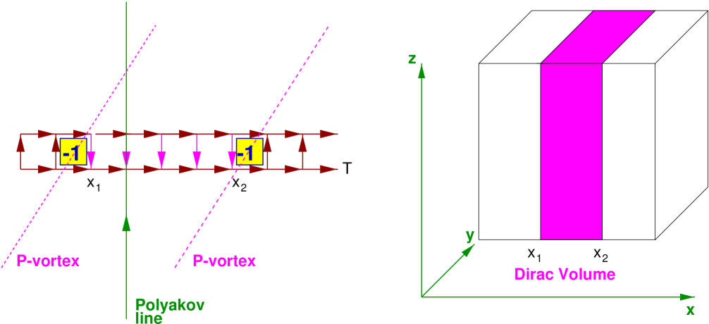
Figure 1: Left: The effect of the transformation (7) on links at fixed $y,z$ and $t=T,1$. Downward pointing time-like links have been multiplied by $-1$. Right: Parallel vortex surfaces created at constant $x_{1},x_{2}$, $t=T$ bound a Dirac volume, closed in the $y,z$ directions by lattice periodicity.

At this point, however, we have to face up to the Gribov copy problem. Center vortices on unprojected lattice configurations are comparatively thick ($\approx$ 1 fm) objects, and the precise “middle” of a vortex core, which P-vortices are supposed to locate, is a little ambiguous. In fact, it is found that if we take two gauge copies $U_{I}$ and $U_{II}$ of the same configuration $U$, gauge-fix each to maximal center gauge and then center project, that the P-vortices in the corresponding projected configurations $Z_{I}$ and $Z_{II}$, although correlated, differ somewhat in position. Thus, a P-vortex plaquette in $Z_{I}$ which is just inside the minimal surface of a given loop $C$, may lie just outside this minimal surface in configuration $Z_{II}$ (for a more detailed discussion and related numerical results, see ref. [3]).

The randomizing effect of small differences in P-vortex locations in $Z$ and $Z^{\prime}$ (which correspond to the same “thick” vortices in $U$ and $U^{\prime}$) will cause the vev $\langle P^{\prime}(x,y,z)P(x,y,z)\rangle$ to differ from $-1$ and $+1$, respectively, inside and outside the region $x\in[x_{1},x_{2}]$. However, if the vortex-finding property is valid, then eq. (9) should hold true when this randomizing effect is factored out. To this end, we generate a set of thermalized SU(2) lattice configurations and, from each configuration, we obtain three configurations consisting of

I.   The original configuration, denoted $U_{I}$.

II.  The original configuration with an inserted vortex, denoted $U_{II}$. In most of our simulations, a thin vortex is inserted by applying the mapping (7), followed by a random (but continuous) gauge transformation $g_{II}$ at every site.

III. A gauge copy of $U_{I}$, denoted $U_{III}$, obtained by applying a random continuous gauge transformation $g_{III}$ to $U_{I}$ at every site.

We then fix each of these configurations to an appropriate adjoint gauge, center project according eq. (2), and compute the ratio

$$G(x)=\frac{\sum_{y,z}\langle P_{I}(x,y,z)P_{II}(x,y,z)\rangle}{\sum_{y,z}\langle P_{I}(x,y,z)P_{III}(x,y,z)\rangle}$$ (10)

where $P_{I},P_{II},P_{III}$ denote Polyakov lines in the corresponding projected configurations, and where the denominator has the effect of factoring out the randomizing (Gribov-copy) effects just mentioned. Then the gauge-fixing + projection procedure has the vortex-finding property only if

$$G(x)=\left\{\begin{array}[]{rl}-1&x\in[x_{1},x_{2}]\cr+1&\mbox{otherwise}\end{array}\right.$$ (11)

3.1 Thin Vortex Insertion, Maximal Center Gauge

For our first test of the VF-property, we have performed the Monte Carlo simulation on a $14^{3}\times 12$ lattice at $\beta=2.3$, and applied a discontinuous gauge transformation (eq. (7) followed by a random continuous gauge transformation) to insert thin vortices as described above. We then fix to maximal center gauge via over-relaxation, as described in ref. [3], center project according to eq. (2), and calculate $G(x)$. The discontinuity in eq. (6) is chosen to lie in the range $x\in[4,10]$.

The result for $G(x)$ is shown in fig. 2. The criterion for the vortex-finding property, eq. (11), appears to be nicely confirmed in this case. Given the successes of our procedure, summarized in the Introduction, in extracting the vortex content of vacuum configurations, the existence of a vortex-finding property was perhaps to be expected. We find that in this case, the existence of Gribov copies in our gauge-fixing procedure does not destroy the VF-property.

Figure 2: Graph of $G(x)$ for configurations with thin inserted vortices ($14^{3}\times 12$ lattice, 380 lattices, $\beta=2.3$). The gauge discontinuity (7) is located in the 3-volume at $x\in[4,10]$, $t=T$.

Instead of inserting vortices via the transformation (7), followed by a random gauge transformation (8), we have also considered vortex insertion by gauge transformations which are smooth in the t-direction up to the discontinuity at $t=T+1$, taking the form

$$g_{V}(x,y,z,t)=\left\{\begin{array}[]{cl}\exp\Bigl{[}i\pi(t-1)\sigma_{3}/T\Bigr{]}&\mbox{for}~{}~{}x\in[x_{1},x_{2}]\cr 1&\mbox{otherwise}\end{array}\right.$$ (12)

and performed simulations for the same parameters as before ($\beta=2.3$, $14^{3}\times 12$ lattice, $[x_{1},x_{2}]=[4,10]$). As in the previous case, the results are consistent with the vortex-finding property in eq. (11).

Apart from our tests here, based on the values of $G(x)$, we would also like to mention some relevant results reported recently by Montero in ref. [14]. Montero, building on the work of ref. [15], constructs classical SU(3) center vortex solutions on a periodic lattice. The stability of the solution is due to the use of twisted boundary conditions, with two dimensions of the periodic lattice chosen much smaller than the two other dimensions. The lattice is fixed to maximal center gauge and then center-projected. It is found that P-vortex plaquettes accurately locate the middle of the classical vortex. This is very interesting independent evidence for the existence of the vortex-finding property of maximal center gauge (in SU(3) gauge theory, in this case).

3.2 Thin Vortex Insertion, Kovács-Tomboulis Procedure

The argument for the vortex-finding property of adjoint gauges, as presented in section 2, explicitly neglects the problem of Gribov copies, and in fact the possibility of gauge-fixing to a unique configuration was an essential step in the argument. Conversely, it follows that the existence of Gribov copies in the gauge fixing procedure might destroy the vortex-finding property, and, as a consequence, the ability of the projection procedure to locate center vortices in thermalized lattice configurations. This appears to be what happens in a modification of our gauge-fixing procedure considered recently by Kovács and Tomboulis [13] (and also noted in ref. [6].)

Kovács and Tomboulis suggest fixing first to the (usual) lattice Landau gauge, before fixing to maximal center gauge via over-relaxation. Of course, if the over-relaxation procedure transformed each configuration to a unique, global maximum of eq. (1) (i.e. if there were no Gribov copies), then a preliminary fixing to lattice Landau gauge could not possibly make a difference to the result. However, the over-relaxation procedure only finds a local maximum of (1). Thus the starting point can make a difference, at least in principle. Kovács and Tomboulis find that with a Landau gauge starting point, center dominance is completely lost in the projected configurations, which appear to have no asymptotic string tension. This fact does not really affect the status of P-vortices, identified by the usual method, as locators of physical objects. That status is well established by the correlation of P-vortices with gauge-invariant observables, and by their scaling properties. In the modified procedure, however, it would appear that some important property, essential for extracting the center vortex content of vacuum configurations, has been lost. From everything that has been said until now, the obvious candidate for this “essential property” is the vortex-finding property.

Figure 3: Graph of $G(x)$ for configurations with a thin inserted vortex. Configurations are first fixed to the Landau gauge, and only then to maximal center gauge ($14^{3}\times 12$ lattice, 260 lattices, $\beta=2.3$). The Dirac volume is the same as in fig. 2.

In fig. 3 we display our results for the observable $G(x)$, in which each configuration $U_{I},U_{II},U_{III}$ is first fixed to Landau gauge, before fixing to maximal center gauge via over-relaxation. The contrast between Figs. 2 and 3 is quite striking; the Kovács-Tomboulis procedure is clearly inconsistent with eq. (11), and seems to have completely lost the vortex-finding property. Only at the boundary of the Dirac volume, where there is a strong local field strength, does $G(x)$ show some effect (although $G(x)>0$ even there). But in the middle of the Dirac volume, $G(x)$ is comparable to its value outside the volume. It seems likely that if the interval $[x_{1},x_{2}]$ were large enough, the middle of the Dirac volume would be indistinguishable from the outside region. Since this modified procedure cannot even identify a thin center vortex inserted into the lattice by hand, there is no reason to expect it to locate the fuzzy, much more diffuse center vortices generated by the gauge theory dynamics.

3.3 Thin Vortex Insertion, Asymmetric Adjoint Gauge

The argument for the vortex-finding property in section 2 did not single out the maximal center gauge in particular; it is possible that other adjoint gauge choices might work just as well. Let us therefore introduce the “Asymmetric Adjoint Gauge”

$$R=\sum_{x}\sum_{\mu}c_{\mu}\Bigl{|}\mbox{Tr}[U_{\mu}(x)]\Bigr{|}^{2}~{}~{}~{}\mbox{is a maximum}$$ (13)

where $c_{\mu}$ is some set of four positive numbers. For an exploratory run at $\beta=2.3$, again on a $14^{3}\times 12$ lattice, we chose a set of values

$$\{c_{1},c_{2},c_{3},c_{4}\}=\{1.0,1.5,0.75,1.0\}$$ (14)

and fixed to the gauge (1) by over-relaxation (without prior Landau gauge-fixing).

Figure 4: Graph of $G(x)$ for configurations with a thin inserted vortex. Configurations are fixed to the asymmetric adjoint gauge with $c_{\mu}=\{1,1.5,0.75,1\}$ ($14^{3}\times 12$ lattice, 380 lattices, $\beta=2.3$). The Dirac volume is the same as in fig. 2.

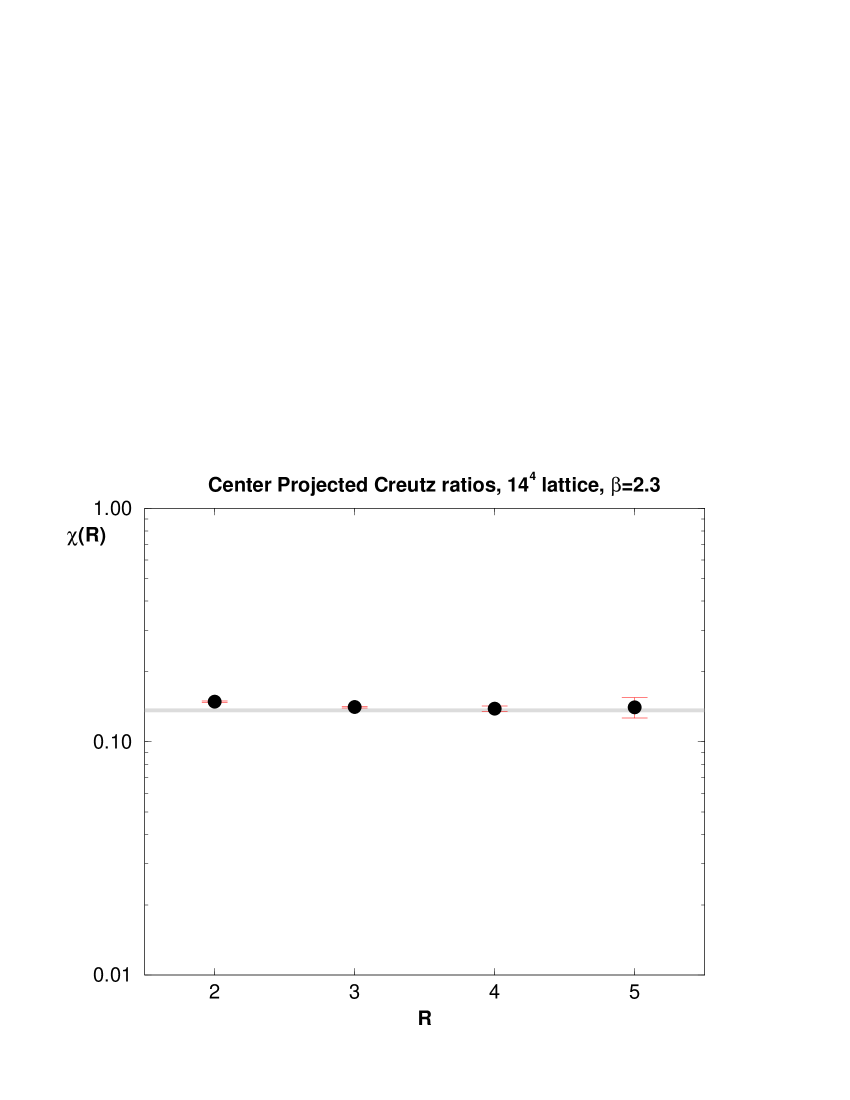
Figure 5: Center dominance for the gauge with $c_{\mu}=\{1,1.5,0.75,1\}$. ($14^{4}$ lattice, $\beta=2.3$.) Solid line shows the value of asymptotic string tension quoted in ref. [16].

The result for $G(x)$ in this new gauge is shown in fig. 4. Once again, the vortex-finding property is satisfied within errorbars. The next question is: Do the corresponding center-projected configurations display center dominance (i.e. do they have the same string tension as the unprojected configuration)? In a run at $\beta=2.3$ on a $14^{4}$ lattice, in the asymmetric adjoint gauge (13), (14), the projected Creutz ratios do, in fact, agree quite well with the asymptotic string tension extracted from gauge-invariant Wilson loops, reported in ref. [16]. The results are shown in fig. 5.

3.4 The Modulus Landau and Adjoint Coulomb Gauges

It was certainly not obvious that the preliminary Landau gauge-fixing, suggested by Kovács and Tomboulis, followed by maximal center gauge-fixing via over-relaxation, would destroy the VF-property (and, as a consequence, center dominance) in the projected configurations. It is also a little surprising that certain choices of adjoint gauge, which would naively seem just as good as maximal center gauge, appear to have similar problems. An example is a “modulus” version of the usual lattice Landau gauge

$$R=\sum_{x}\sum_{\mu}\Bigl{|}\mbox{Tr}[U_{\mu}(x)]\Bigr{|}~{}~{}~{}\mbox{is a maximum}$$ (15)

which is also an adjoint gauge, as defined by the conditions set out in section 2. We believe, on the basis of the argument in section 2, that if $R$ could be fixed to a unique global maximum then this gauge would also have the VF-property, and the projected configurations would exhibit center dominance. However, as with maximal center gauge, the only known gauge-fixing techniques are simulated annealing and over-relaxation, and these are both plagued with Gribov copies. So the only way of testing the vortex-finding property, and center dominance, is numerically.

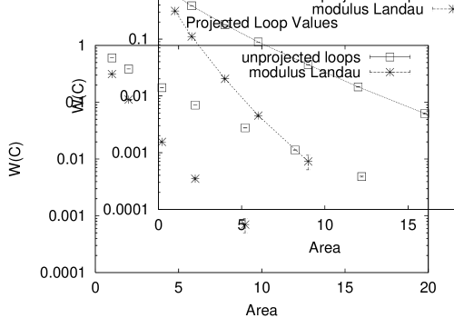
Figure 6: Center-projected Wilson loops vs. Area in modulus Landau gauge, for square $R\times R$ and rectangular $R\times(R+1)$ loops, at $\beta=2.3$ on a $12^{4}$ lattice. Unprojected Wilson loop values are also shown for comparison.

We have used over-relaxation at $\beta=2.3$ to fix to the modulus Landau gauge. In this case, the falloff with area of the projected Wilson loops appears to be much faster than that of the unprojected loops, as seen in fig. 6; center dominance is clearly lost.

Figure 7: Numerator $N(x)$ (eq. (16)) of the ratio $G(x)$, for modulus Landau gauge ($14^{3}\times 12$ lattice, 380 lattices, $\beta=2.3$). The Dirac volume is the same as in fig. 2.

The corresponding values for $G(x)$ in modulus Landau gauge have very large errorbars, and this is simply because both the numerator and denominator in eq. (10) have values which are, within errorbars, consistent with zero. Results for the product in the numerator

$$N(x)={1\over L^{2}}\sum_{y,z}\langle P_{I}(x,y,z)P_{II}(x,y,z)\rangle$$ (16)

are shown in fig. 7, where $L$ ($=14$) is the lattice length in the $y,z$-directions. It is clear that there is in this case a total loss of the vortex-finding property. In contrast to the Kovács-Tomboulis case, in which $G(x)$ was positive irrespective of linking to the inserted vortex, in this case $G(x)$ seems to be essentially $0/0$, irrespective of linking number. But just as in the Kovács-Tomboulis case, the failure of center dominance in the projected configurations is associated with a corresponding loss of the vortex-finding property.

Figure 8: Graph of $G(x)$ for configurations with thin inserted vortices ($14^{3}\times 12$ lattice, 110 lattices, $\beta=2.3$) in modulus Landau gauge. In this case, the lattice is first fixed to maximal center gauge, before fixing via over-relaxation to modulus Landau gauge.

Since the modulus Landau gauge should be a perfectly good adjoint gauge, the failure of the vortex-finding property in this case must be attributed to the Gribov copy problem. This impression is strengthened when one compares the rms value of $a_{0}$, where

$$U_{\mu}=a_{0}I+i\vec{a}\cdot\vec{\sigma}$$ (17)

in both the modulus Landau and maximal center gauges. We find that $a_{0}^{rms}=0.76$ in modulus Landau gauge, vs. $a_{0}^{rms}=0.86$ in maximal center gauge, at $\beta=2.3$, and that is a surprisingly large discrepancy, in view of the fact that both gauges are, in some sense, trying to bring links close to center elements. This suggests trying out a variation of the Kovacs-Tomboulis procedure: Perhaps modulus Landau gauge-fixing could be improved, if we first fix to maximal center gauge, and then fix to modulus Landau gauge via over-relaxation.

It turns out that a preliminary gauge-fixing to maximal center gauge restores both center dominance and the vortex-finding property. For center dominance, we find that the Creutz ratios, at $\beta=2.3$, are clustered near $\chi[R,R]\approx 0.14$, quite close to the asymptotic string tension obtained on unprojected lattices. The result for $G(x)$ is shown in fig. 8; it is similar to what we previously found for maximal center gauge and the asymmetric Landau gauge.

Once again, the presence or absence of the vortex-finding property is associated with the presence or absence of center dominance in the projected configurations.

Figure 9: Numerator $N(x)$ (eq. (16)) of the ratio $G(x)$, for adjoint Coulomb gauge ($14^{3}\times 12$ lattice, 180 lattices, $\beta=2.3$). The Dirac volume is the same as in fig. 2.

In section 3.3 we studied the asymmetric adjoint gauge, with a moderate variation of $c_{\mu}$ between $0.75$ and $1.5$. It is also of interest to look at limiting cases of this gauge, where the ratios of some of the $c_{\mu}$’s tend to zero or infinity. A particular example we have investigated is the adjoint Coulomb gauge, in which

$$\{c_{1},c_{2},c_{3},c_{4}\}=\{1.0,1.0,1.0,0.0\}$$ (18)

Center dominance is lost in this gauge also, although the disagreement between full and projected string tensions is not quite as bad as in modulus Landau gauge without preconditioning. Creutz ratios in the projected configurations at $\beta=2.3$ cluster around $\chi_{proj}(R,R)\approx 0.18$, whereas the full asymptotic string tension is around $\sigma a^{2}=0.135$.

As in modulus Landau gauge, the loss of center dominance in adjoint Coulomb gauge is accompanied by a breakdown of the vortex-finding property, as seen from a plot of the numerator (16) in fig. 9. The qualitative difference between adjoint Coulomb gauge, and the asymmetric adjoint gauge studied in section 3.3, may be connected with the fact that adjoint Coulomb gauge is not really an adjoint gauge, as defined in section 2. Our third criterion for adjoint gauges is that link variables should be brought close to center elements. What we find instead, at $\beta=2.3$, is that while the rms value $a_{0}^{rms}$ for spacelike links is $0.89$, the corresponding rms value for timelike links is only $0.50$ (and this is identical to the rms values of the other three components $a_{k}^{rms}$. Thus, while spacelike links do indeed fluctuate near center elements, the timelike links do not, and the “close-to-center” criterion is violated. This criterion for adjoint gauges will be further discussed in section 3.6.

3.5 Thicker Inserted Vortex, Maximal Center Gauge

All of the inserted vortices so far are thin vortices; the vortex core has a thickness of one lattice spacing. On the other hand, the vortices generated dynamically by the gauge theory seem to be rather thick objects, with core widths on the order of one fermi. It is therefore of interest to see if an inserted vortex with a somewhat thickened core can also be identified on the projected lattice.

In our previous examples, the $-1$ discontinuity in the vortex-creating transformation $g_{V}$ begins and ends abruptly at $x=x_{1}$ and $x=x_{2}$. To create a vortex core several lattice units thick in the x-direction, we simply make the transition from the $-1$ discontinuity to $+1$ continuity more gradual. This is done by replacing the mapping in eq. (7) by

$$U_{4}(x,y,z,T)\rightarrow U_{4}(x,y,z,T)\exp[i\alpha(x)\sigma_{3}]$$ (19)

where $\alpha(x)$ interpolates smoothly from $\alpha(x)=0$ outside the Dirac volume, to $\alpha(x)=\pi$ inside the Dirac volume.

We make the choice for $\alpha(x)$ shown in Table 1 on an $18^{3}\times 8$ lattice, followed by a random gauge transformation, to obtain configurations $U_{II}$.

x 1 2 3 4 5 6 7 8 9 10 11 12 13 14 15 16 17 18 $\alpha$ 0 0 0 ${\pi\over 5}$ ${2\pi\over 5}$ ${3\pi\over 5}$ ${4\pi\over 5}$ $\pi$ $\pi$ $\pi$ $\pi$ ${4\pi\over 5}$ ${3\pi\over 5}$ ${2\pi\over 5}$ ${\pi\over 5}$ 0 0 0

Table 1: Thick vortex core: $\alpha(x)$ in eq. (19).

Maximal center gauge-fixing and center projection are carried out, and $G(x)$ is calculated, with results shown in fig. 10 (obtained at $\beta=2.3$). Once again the vortex-finding property is quite evident, with $G(x)$ interpolating smoothly from $+1$ to $-1$ across the vortex core.

Figure 10: $G(x)$ computed for thicker vortices on an $18^{3}\times 8$ lattice, 380 lattices, $\beta=2.3$.

3.6 The “Close-to-Center” Criterion

All of the gauges we have considered have the property of bringing most link variables close to the $\pm I_{2}$ center variables. This was listed as the third criterion of an adjoint gauge in section 2, and we should now explain the rationale behind this criterion.

The picture which is implied by the numerical studies [1$-$11] is that thermalized SU(2) lattice configurations have the form

$$U=G_{V}\circ U_{NC}$$ (20)

where $G_{V}$ is an operator creating center vortices responsible for confinement, while $U_{NC}$ is a non-confining lattice background. The operator $G_{V}$ is a “smoothed” discontinuous gauge transformation; i.e. it is has the form of a discontinuous gauge transformation, away from vortex cores. In an adjoint gauge which has the vortex-finding property, center projection should locate the approximate position of vortices created by $G_{V}$.

There is no guarantee, however, that gauge-fixing + center projection will not also produce, in addition to the P-vortices associated with $G_{V}$, a lot of other extraneous P-vortices with no physical content, nor is there any obvious reason that these extraneous P-vortices should be independent of the choice of adjoint gauge. This is the motivation for introducing, in the definition of adjoint gauges, a “close-to-center” requirement.

In maximal center gauge (or any other adjoint gauge), not all links are close to center elements, even at large $\beta$; some links lying in the middle of center vortices must deviate very substantially from $\pm I_{2}$. This deviation from the center elements is necessary, in order that a projected plaquette can equal $-1$, while the corresponding gauge-invariant plaquette on the unprojected lattice is close to $+1$ at weak coupling (cf. [18]). The aim of the “close-to-center” requirement is that links should deviate substantially from center elements only where they must do so, i.e. in the cores of vortices created by $G_{V}$; elsewhere the gauge-fixing condition should force links to fluctuate in the vicinity of $\pm I_{2}$. This criterion is, of course, most obvious in maximal center gauge.

Let MC denote maximal center gauge, and AG denote another adjoint gauge which (i) has the VF-property, and (ii) has most links close to center elements, except in the middle of center vortices. We can then argue that, away from vortex interiors, the center-projected configurations $Z_{MC}$ and $Z_{AG}$ will be $Z_{2}$ gauge-equivalent. Let $U^{\prime}_{MC},U^{\prime}_{AG}$ represent a thermalized configuration $U$ fixed to the MC and AG gauges, respectively. We can write

$$U^{\prime}_{MC} = Z_{MC}U^{\prime\prime}_{MC}~{}~{}~{}\mbox{where}~{}~{}~{}U^{\prime\prime}_{MC}=\mbox{signTr}[U^{\prime}_{MC}]U^{\prime}_{MC}$$

$$U^{\prime}_{AG} = Z_{AG}U^{\prime\prime}_{AG}~{}~{}~{}~{}\mbox{where}~{}~{}~{}U^{\prime\prime}_{AG}~{}=\mbox{signTr}[U^{\prime}_{AG}]U^{\prime}_{AG}$$ (21)

where the product and sign trace operations are of course performed link by link. Because $U^{\prime}_{MC}$ and $U^{\prime}_{AG}$ are gauge-equivalent, we have

$$U^{\prime}_{AG} = (zg)\circ U^{\prime}_{MC}$$ (22)

$$= (z\circ Z_{MC})(g\circ U^{\prime\prime}_{MC})$$

where $z$ is a $Z_{2}$ gauge transformation, and $\mbox{Tr}[g]\geq 0$. Away from vortex interiors, most links in $U^{\prime}_{MC}$ and $U^{\prime}_{AG}$ are close to $\pm I_{2}$ at large $\beta$, which implies that $g\circ U^{\prime\prime}_{MC}\approx\pm I_{2}$ are also close to center elements. Combining this with the fact that $U^{\prime\prime}_{MC}\approx+I_{2}$ and $\mbox{Tr}[g]>0$, we deduce that $g(x)\approx g(x+\mu)$ in this region, and therefore $g\circ U^{\prime\prime}_{MC}\approx+I_{2}$. We can then identify

$$U^{\prime\prime}_{AG} = g\circ U^{\prime\prime}_{MC}$$

$$Z_{AG} = z\circ Z_{MC}$$ (23)

According to this argument, $Z_{AG}$ and $Z_{MC}$ are $Z_{2}$ gauge-equivalent, away from the vortex interior.

Inside a vortex core, $U^{\prime\prime}_{MC}$ is not necessarily close to the identity, so $Z_{AG}$ and $Z_{MC}$ are not necessarily gauge-equivalent. This implies that there will in general be some variation in P-vortex location among different adjoint gauges (and among Gribov copies in the same adjoint gauge), associated with the finite width of the center vortex core. But apart from this local variation, the vortices found by two adjoint gauges should be basically the same, providing that both gauges have the vortex-finding property, and providing that the links in both gauges are close to center elements everywhere except where they must strongly deviate, i.e. in the core of vortices created by $G_{V}$. How well this “close-to-center” requirement is actually fulfilled, in different adjoint gauges with the vortex-finding property, is a topic which has not yet been studied in any detail.

3.7 Speculations about Cooling and Smoothing

If maximal center gauge + center projection is applied to cooled configurations, then the projected string tension is drastically reduced after only a few cooling steps (similar results are found for RG-smoothed configurations) [3]. But it was also found in ref. [3] that the cores of thick center vortices, whose approximate location is identified before cooling, also expand considerably after only a few cooling steps, as measured by the one-vortex to zero-vortex loop ratio $W_{1}(C)/W_{0}(C)$.

Center vortices in thermalized lattices have been found to be rather thick, “fuzzy” objects, which percolate throughout the lattice. It appears that, after a few cooling steps, the vortex cores overlap so much that there is virtually no region of the lattice which is not part of a vortex core. In view of the second caveat (“Vortex Cores”) in section 2, it is then not so surprising that the maximal center gauge + center projection procedure is unable to extract the locations of these very fat, highly overlapping objects (although the method seems to have no trouble finding thin, inserted vortices after a few cooling steps).

3.8 Laplacian Center Gauge

According to our argument in section 2, an adjoint gauge without the Gribov copy problem is guaranteed to have the vortex-finding property, at least for thin inserted vortices where vortex width is only one lattice spacing. Such a gauge was invented recently by Alexandrou, D’Elia, and de Forcrand [17]; it is known as the “Laplacian Center Gauge.”

To fix to Laplacian center gauge, one finds the eigenvectors $\vec{u}(x),\vec{v}(x)$ corresponding to the two lowest eigenvalues of of the covariant lattice Laplacian

$$\Delta_{xy}^{ab}=2D\delta_{xy}\delta^{ab}-\sum_{\pm\mu}U_{A,\pm\mu}^{ab}(x)\delta_{x\pm\mu,y}$$ (24)

where

$$U^{ab}_{A,\mu}=\frac{1}{2}\mbox{Tr}[U_{\mu}\sigma^{a}U_{\mu}^{\dagger}\sigma^{b}]$$ (25)

are matrix elements of the link variables in the adjoint representation. The gauge transformation which takes the lattice configuration into Laplacian center gauge is the transformation which rotates $\vec{u}(x)$ to lie in the 3-direction, and $\vec{v}(x)$ to lie in the 1-3 plane, at every site $x$. This procedure is free of Gribov copies, and it was found in the second reference of [17] that there is agreement between the asymptotic string tensions on the full and projected lattices, at least at the coupling $\beta=2.4$ used there. Although Laplacian center gauge does not involve directly maximizing a functional (as in eq. (4)), it does satisfy all three conditions below (4), and thus qualifies as an adjoint gauge.

We have checked the VF-property for Laplacian center gauge as before; i.e. for a thin inserted vortex on the same lattice as in fig. 2, at $\beta=2.3$. The somewhat startling result is that the condition

$$G(x)=\left\{\begin{array}[]{rl}-1&x\in[4,10]\cr+1&\mbox{otherwise}\end{array}\right.$$ (26)

is satisfied by the numerical data exactly. In other words, there are no errorbars at all; every configuration gives the same result for $G(x)$. Fixing to Landau gauge, prior to Laplacian center gauge, makes no difference to this result.

In fact, the absence of errorbars on $G(x)$ in Laplacian center gauge is simply a confirmation of the reasoning in sections 2 and 3. As noted above, the VF-property is guaranteed in this gauge, at least for thin vortices. We have also argued, in section 3, that any deviation from eq. (9) must be due to small variations in P-vortex location, from one Gribov copy to another, and these variations are responsible for the statistical fluctuations in $G(x)$. Eliminating Gribov copies eliminates in turn these statistical fluctuations, and the VF-property for Laplacian center gauge is seen in the most compelling way.

Laplacian center gauge is not quite as “close to center” as maximal center gauge. We find, for example, that the rms value of $a_{0}=\mbox{Tr}[U]/2$ at $\beta=2.3$ is approximately $a_{0}^{rms}=0.86$ in maximal center gauge, but only $a_{0}^{rms}=0.82$ in Laplacian center gauge. There are also more P-vortex plaquettes in the projected Laplacian configurations; ref. [17] reports an excess in P-vortex plaquettes of about $11$%, at $\beta=2.4$, as compared to maximal center gauge. The greater number of P-vortex plaquettes found in Laplacian center gauge does not affect the asympotic string tension of projected configurations, and can probably be attributed to one (or both) of two sources: (i) a roughening of the P-vortex surface; (ii) some extraneous “small” P-vortices, unconnected to the single large vortex responsible for confinement, which is found [9] to percolate through the entire lattice. Either of these effects could modify the projected Creutz ratios at short distances, while preserving the asymptotic string tension. This may explain the slightly delayed approach of projected Creutz ratios to their asymptotic value, relative to previous results in maximal center gauge.

Alexandrou et al. in ref. [17] also suggest an alternative method for identifying vortices via Laplacian center gauge, which is based on locating certain gauge-fixing ambiguities, rather than center projection. We have not yet investigated this method; it would be interesting to know if our argument for the vortex-finding property in adjoint gauges can also be applied in this alternative framework.

4 Conclusions

Gauge-fixing has had a bad reputation, in connection with studies of the confinement mechanism. One is justifiably suspicious of any calculation which depends in an essential way on some special gauge choice, particularly if the physical motivation of that special gauge choice is unclear. In this article we hope to have dispelled some of that suspicion, at least in connection with maximal center and related gauges. Center vortices are created by discontinuous gauge transformations, which of course make no reference to any particular gauge condition. We have argued above that in maximal center gauge $-$ and in an infinite class of other adjoint gauges $-$ such discontinuous transformations are squeezed to the identity everywhere except on Dirac volumes, whose locations (together with those of the associated vortices) are then revealed upon center projection. This is the “vortex-finding property” which motivates the use of adjoint gauges, and it explains how adjoint gauge-fixing, combined with center projection, can extract the vortex content of thermalized lattice configurations.

While we think it likely that every adjoint gauge, as defined in section 2, has the VF-property, this is certainly not true of every gauge-fixing procedure. The argument for the VF-property assumed a complete and unique adjoint gauge-fixing, but unfortunately the standard over-relaxation and simulated annealing methods are plagued by Gribov copies. This is a large loophole in the argument for vortex-finding, and in certain cases, e.g. the Kovács-Tomboulis procedure, the Gribov copy problem is apparently severe enough to destroy the VF-property.

It is not clear, at present, why the Gribov problem destroys the VF-property only in some gauge-fixing procedures, but not in others. What does seem clear, however, is that the vortex-finding property, and the center dominance of projected configurations, go hand-in-hand. Maximal center gauge, asymmetric adjoint gauge, modulus Landau gauge with maximal center preconditioning, and Laplacian center gauge all have the VF-property, and all exhibit center dominance. Conversely, in the (i) Kovács-Tomboulis procedure, (ii) modulus Landau gauge without preconditioning, and (iii) adjoint Coulomb gauge, the VF-property is lost, and in none of these cases is there center dominance in the projected configurations.

We conclude with a sort of tautology: To find center vortices, one must use a procedure with the vortex-finding property. If the gauge-fixing + projection procedure doesn’t have the VF-property, or if that property is destroyed by some modification (e.g. by Landau gauge preconditioning), then center vortices are not correctly identified on thermalized lattices, and center dominance in the projected configuration is lost. This fact does not call into question the physical relevance of P-vortices found by our usual procedure (which has the vortex-finding property); that relevance is well established by the strong correlation that exists between these objects and gauge-invariant observables. Ideally, potential problems due to Gribov copies could be avoided altogether by a gauge-fixing procedure which fixes to a unique adjoint link configuration. Laplacian center gauge [17] appears to be an example of just such a procedure.

Acknowledgements

We thank Phillipe de Forcrand for discussions. J.G. is happy to acknowledge the hospitality of the high-energy theory group at the Niels Bohr Institute, where much of this work was carried out.

Our research is supported in part by Fonds zur Förderung der Wissenschaftlichen Forschung P11387-PHY (M.F.), the U.S. Department of Energy under Grant No. DE-FG03-92ER40711 (J.G.), and the Slovak Grant Agency for Science, Grant No. 2/4111/97 (Š. O.).

References

- [1] L. Del Debbio, M. Faber, J. Greensite, and Š. Olejník, Phys. Rev. D55 (1997) 2298, hep-lat/9610005.
- [2] L. Del Debbio, M. Faber, J. Greensite, and Š. Olejník, in New Developments in Quantum Field Theory, ed. Poul Henrik Damgaard and Jerzy Jurkiewicz (Plenum Press, New York–London, 1998) 47, hep-lat/9708023.
- [3] L. Del Debbio, M. Faber, J. Giedt, J. Greensite, and Š. Olejník, Phys. Rev. D58 (1998) 094501, hep-lat/9801027.
- [4] M. Faber, J. Greensite, and Š. Olejník, JHEP 9901 (1999) 008, hep-lat/9810008.
-
[5]
M. Faber, J. Greensite, and
Š. Olejník, Phys. Rev. D57 (1998) 2603, hep-lat/9710039;
M. Faber, J. Greensite, and Š. Olejník, Acta. Phys. Slov. 49 (1999) 177, hep-lat/9807008. - [6] Ph. de Forcrand and M. D’Elia, Phys. Rev. Lett. 82 (1999) 4582, hep-lat/9901020.
- [7] K. Langfeld, H. Reinhardt, and O. Tennert, Phys. Lett. B419 (1998) 317, hep-lat/9710068.
- [8] M. Engelhardt, K. Langfeld, H. Reinhardt, and O. Tennert, hep-lat/9904004; and Phys. Lett. B452 (1999) 301, hep-lat/9805002.
- [9] R. Bertle, M. Faber, J. Greensite, and Š. Olejník, JHEP 9903 (1999) 019, hep-lat/9903023.
-
[10]
B. Bakker, A. Veselov, and M. Zubkov, hep-lat/9902010;
M. Chernodub, M. Polikarpov, A. Veselov, and M. Zubkov, Nucl. Phys. Proc. Suppl. 73 (1999) 575, hep-lat/9809158. - [11] T. Kovács and E. Tomboulis, Lattice 99 Proceedings, hep-lat/9908031.
- [12] J. Ambjørn, J. Giedt, and J. Greensite, hep-lat/9907021.
- [13] T. Kovács and E. Tomboulis, hep-lat/9905029.
- [14] A. Montero, hep-lat/9906010.
- [15] A. Gonzalez-Arroyo and A. Montero, Phys. Lett. B442 (1998) 273, hep-th/9809037.
- [16] G. Bali, C. Schlichter, and K. Schilling, Phys. Rev. D51 (1995) 5165, hep-lat/9409005.
- [17] C. Alexandrou, M. D’Elia, and Ph. de Forcrand, Lattice 99 Proceedings, hep-lat/9907028; and hep-lat/9909005.
- [18] K. Langfeld and H. Reinhardt, Phys. Rev. D55 (1997) 7993, hep-lat/9703012.