Light Hadron Weak Matrix Elements

Abstract

Recent developments in lattice QCD calculation of weak matrix elements involving light quarks are described. We focus on four topics: $B_{K}$ with the Kogut-Susskind and Wilson quark actions, $\Delta I=1/2$ rule, proton decay matrix elements and the application of domain wall QCD to calculation of weak matrix elements.

1 Introduction

The kaon bag parameter $B_{K}$, which is required for constraining the CP violation parameter in the Cabibbo-Kobayashi-Maskawa matrix from experiment, has been successfully calculated with the Kogut-Susskind(KS) quark action, taking advantage of its ${\rm U_{A}}(1)$ chiral symmetry[1]. A recent systematic calculation of $B_{K}$ with high statistics[2], however, reveals that the systematic uncertainties in the perturbative renormalization factors to connect lattice and continuum operators have sizable magnitude, which indicates the necessity of non-perturbative renormalization. For the calculation of $B_{K}$ with the Wilson quark action we have to deal with the operator mixing problem caused by the explicit chiral symmetry breaking in the action, which turned out to be not effectively treated by perturbation theory[3]. Several non-perturbative methods have been proposed to control the operator mixing.

The CP conserving $K\rightarrow\pi\pi$ decay amplitudes give an intriguing testing ground for lattice QCD calculations. It would be exciting to be able to show that QCD explains the $\Delta I=1/2$ rule: $A_{0}/A_{2}\approx 22$ where $A_{0,2}=A(K\rightarrow\pi\pi[I=0,2])$. Although studies of $K\rightarrow\pi\pi$ decay amplitudes with lattice QCD were initiated a decade ago, little progress has been achieved since then. Recent work on the one-loop calculation of $K\rightarrow\pi\pi$ decay amplitudes using chiral perturbation theory(ChPT)[4, 5], however, provides some important information about the lattice results.

In lattice QCD studies for the proton decay amplitude $\langle\pi^{0}|{\cal O}^{{{B}{/}}}|p\rangle$, pioneering work estimated it from the matrix element $\langle 0|{\cal O}^{{{B}{/}}}|p\rangle$ with the aid of the chiral lagrangian[6, 7], which were followed by the direct measurement of $\langle\pi^{0}|{\cal O}^{{{B}{/}}}|p\rangle$[8]. The results showed an unexpectedly large discrepancy between these two methods: the direct method yielded a two or three times smaller value than the indirect one. This peculiar feature was confirmed by JLQCD last year[9]. At this conference, however, JLQCD[10] pointed out that the calculational method in refs.[8, 9] was wrong, and presented the correct estimate of the proton decay amplitudes with the direct method.

The domain wall quark formulation in lattice QCD[11, 12] potentially has superior features over the Wilson and KS quark actions: realization of the chiral limit on arbitrary number of flavors without fine tuning. Recent simulation results for $B_{K}$ show a good chiral behavior[13], which encourages us to apply the domain wall quark to the calculation of weak matrix elements. Some progress has been made this year numerically and theoretically.

This article is organized as follows. In Sec. 2 we present the $B_{K}$ results with the KS and Wilson quark actions. From the examination of the systematic errors in the KS result we explain the reason why the non-perturbative renormalization is necessary. The present status of the non-perturbative renormalization method is also discussed. Results for the $K\rightarrow\pi\pi$ decay amplitudes are presented in Sec. 3, where we focus on the one-loop effects of ChPT. In Sec. 4 we describe an essential advance on the calculation of the proton decay matrix elements. This year’s progress on the calculation of weak matrix elements with the domain wall QCD is explained in Sec. 5. Our conclusions are summarized in Sec. 6. Results for structure functions have been reviewed by Petronzio[14].

2 $B_{K}$

2.1 $B_{K}$ with the KS quark action

The $K$ meson $B$ parameter is defined by

$$B_{K}=\frac{\langle{\bar{K}}^{0}|\bar{s}\gamma_{\mu}(1-\gamma_{5})d\cdot\bar{s}\gamma_{\mu}(1-\gamma_{5})d|K^{0}\rangle}{\frac{8}{3}\langle{\bar{K}}^{0}|\bar{s}\gamma_{\mu}\gamma_{5}d|0\rangle\langle 0|\bar{s}\gamma_{\mu}\gamma_{5}d|K^{0}\rangle},$$ (1)

for which we quote results in the naive dimensional regularization(NDR) scheme at the renormalization scale 2GeV. In the ratio of eq.(1) the fluctuations are largely canceled between the numerator and the denominator, which enable us to easily achieve high statistical accuracy. Taking advantage of this virtue, we have had control over the systematic errors step by step. As of this conference $B_{K}$ is the weak matrix element with which we have had the most success.

Figure 1 presents a recent result for a systematic quenched $B_{K}$ calculation performed by JLQCD employing seven values of lattice spacing with $m_{d}=m_{s}$[2]. The non-local weak four-fermi operator is constructed either in gauge invariant way with insertion of the link variables (${\cal O}_{\rm inv}$) or in non-invariant way without link variables in Landau gauge (${\cal O}_{\rm non-inv}$). Each operator is perturbatively matched to the operator in the continuum NDR scheme at the scale $q^{*}=1/a$ employing tadpole improvement. The value of $B_{K}$ at $\mu=2$GeV is obtained via a two-loop renormalization group running from $\mu=1/a$GeV.

Figure 1: Quenched $B_{K}({\rm NDR,2GeV})$ with the KS quark action as a function of $m_{\rho}a$. See text for the solid and dashed lines. Domain wall fermion results will be explained in Sec. 5.

The statistical error is $0.1\%$ at the largest lattice spacing and gradually increasing to $1.2\%$ at the smallest one. Let us examine conceivable systematic errors in order. (i) Quark mass dependence: $B_{K}$ at the physical kaon point is accessible with interpolation, not extrapolation, which means the interpolated value is strongly robust against the choice of fitting function. (ii) Finite size effects: Finite size studies at $\beta=6.0$ and $6.4$ show that the magnitude of the size dependence decreases to less than $0.5\%$ for $L\geq 2.2$fm. The spatial size is kept larger than $L\simeq 2.3$fm at all $\beta$. (iii) Scaling violation: The five data points below $m_{\rho}a\simeq 0.6$ for each operator are consistent with $O(a^{2})$ scaling behavior expected theoretically[15]. A quadratic fit of the five points(dashed lines in Fig 1) gives a value at the continuum limit $B_{K}=0.616(5)$ for ${\cal O}_{\rm non-inv}$ and $0.580(5)$ for ${\cal O}_{\rm inv}$. This $7\sigma$ discrepancy raises the question of what causes this difference. (iv) $O(\alpha^{2})$ uncertainties: As seen in the matching procedure of ${\cal O}_{\rm inv,non-inv}$ to the continuum operator, their difference $\Delta B_{K}$ should be of not only $O(a^{2})$ but also $O(\alpha^{2})$. Figure 2 illustrate that the difference is well described by the function $\Delta B_{K}=b_{1}(m_{\rho}a)^{2}+b_{2}(\alpha_{\overline{\rm MS}}(q^{*}))^{2}$ below $m_{\rho}a\simeq 0.6$, which suggests that a $\alpha_{\overline{\rm MS}}^{2}$ term should be incorporated in the fit of $B_{K}$. An attempt to simultaneously fit $B_{K}$ for both operators is shown in Fig. 1(solid lines), which yields $B_{K}=0.628(42)$ in the continuum limit(cross). This $7\%$ error, which is roughly 10 times larger than those with naive quadratic fit, reflects the magnitude of the $O(\alpha^{2})$ uncertainties in the operator matching procedure. To eliminate the $O(\alpha^{2})$ uncertainties, it would be necessary to adopt the non-perturbative renormalization method. (v) Quenching effects: In 1996 the OSU group studied the dynamical quark effects on $B_{K}$ employing three ensembles of gauge configurations at $a^{-1}\approx 2$GeV: $N_{f}=0$ at $\beta=6.05$, $N_{f}=2$ at $\beta=5.7$ and $N_{f}=4$ at $\beta=5.4$[16]. They found that $B_{K}$ with $N_{f}=3$ is $5\pm 2\%$ larger than the quenched value. However, it is hard to assume this number as the dynamical quark effects in the continuum limit: we cannot exclude the possibility that the scaling violation of $B_{K}$ in full QCD might be different from the quenched case. This fact compels us to perform the systematic calculation of $B_{K}$ in full QCD varying the lattice spacing and the dynamical quark mass. (vi) Degenerate quark mass $m_{s}=m_{d}$: For $B_{K}$ in the quenched QCD there is a divergent chiral logarithm as $m_{d}\rightarrow 0$ in the chiral expansion of ChPT[17, 4]. We can investigate the $m_{s}\neq m_{d}$ case only in the full QCD.

Figure 2: Difference of $B_{K}({\rm NDR,2GeV})$ between ${\cal O}_{\rm inv}$ and ${\cal O}_{\rm non-inv}$ as a function of $m_{\rho}a$.

The next step toward the precise determination of $B_{K}$ is the control of the $O(\alpha^{2})$ uncertainties. We also note that the systematic full QCD calculation of $B_{K}$ with $m_{s}\neq m_{d}$ is now feasible in view of the performance of the current full QCD simulations[18].

2.2 Non-perturbative renormalization

A naive non-perturbative renormalization method is to copy what is done in perturbative renormalization in a non-perturbative way[19]. The renormalization condition in the momentum-space subtraction scheme (MOM) for a certain operator is provided by imposing that the off-shell quark matrix element in a fixed gauge should coincide with their tree level value. For example, if we consider the bilinear operator ${\cal O}_{\Gamma}={\bar{\psi}}\Gamma\psi$, the condition is given by $Z_{\Gamma}(g_{0},\mu a)\langle q(p)|{\cal O}_{\Gamma}|q(p)\rangle|_{p^{2}=\mu^{2}}=\langle q(p)|{\cal O}_{\Gamma}|q(p)\rangle_{\rm tree},$ where $\Gamma$ denotes Dirac matrices and $p$ is the off-shell quark momentum. In non-perturbative renormalization on the lattice, the matrix element $\langle q(p)|{\cal O}_{\Gamma}|q(p)\rangle$ is constructed with the vertex and wave functions obtained from the Fourier transformed quark Green functions in Landau gauge. This method, which we refer to as NPMOM method hereafter, is expected to work if we can find the appropriate region for the external quark momentum $\Lambda_{\rm QCD}\ll p\ll a^{-1}$ to avoid the non-perturbative contributions and the cut-off effects simultaneously.

The NPMOM method has been actively being pursued for various operators in different actions[20, 21, 22, 23, 24]. The studies, however, reveal that it is not a trivial task to find the appropriate region of $p$: it depends on each operator strongly; moreover, it is hard to find it for some operators. At the present stage it is not clear to what extent the non-perturbative contaminations and the cut-off effects can be controlled quantitatively. Another concern is the issue of Gribov copies in the Landau gauge fixing. We have no definite way to estimate the ambiguities induced by the choice of Gribov copies.

The technical difficulties in the NPMOM method can be entirely overcome by another non-perturbative method that uses the Schrödinger functional(SF) as the renormalization scheme[25]. The SF scheme is essentially a finite-volume renormalization technique. QCD is considered in a finite space-time volume of physical size $L$ in all directions, where all renormalized quantities are defined at scale $\mu=1/L$. A change of the lattice size at fixed bare parameters is a change of the renormalization scale. For the bilinear operator $\bar{\psi}\Gamma\psi$ a possible choice of the renormalization condition is $Z_{\Gamma}(g_{0},L/a)=c\sqrt{f_{\rm ext}}/f_{\Gamma}(t)|_{t=L/2},$ where $f_{\Gamma}(t)=\int d^{3}{\vec{y}}d^{3}{\vec{z}}\langle{\bar{\psi}_{f}}({\vec{x}},t)\Gamma\psi_{f^{\prime}}({\vec{x}},t){\bar{\zeta}}_{f^{\prime}}({\vec{y}},0)\Gamma\zeta_{f}({\vec{z}},0)\rangle$ and $f_{\rm ext}\hfill=\hfill\int d^{3}{\vec{y}}^{\prime}d^{3}{\vec{z}}^{\prime}d^{3}{\vec{y}}d^{3}{\vec{z}}\langle{\bar{\zeta}}_{f}^{\prime}({\vec{y}}^{\prime},L)\Gamma\zeta_{f^{\prime}}^{\prime}({\vec{z}}^{\prime},L)\\ {\bar{\zeta}}_{f^{\prime}}({\vec{y}},0)\Gamma\zeta_{f}({\vec{z}},0)\rangle$ with $f$, $f^{\prime}$ the flavor. $\zeta,\dots,{\bar{\zeta}}^{\prime}$ denote the boundary quark fields at $t=0$ and $L$ with zero spatial momentum projection. The constant $c$ in the renormalization condition is properly chosen such that $Z_{\Gamma}=1$ at tree-level.

There are three main advantages in the SF scheme. (i) Gauge invariance: It is not necessary to fix the gauge. (ii) Mass independent renormalization: This scheme allows us to perform numerical simulations at zero quark mass. We can specify the boundary conditions such that the lowest eigenvalue of the free Dirac operator is lifted by a gap of order $1/L$ at vanishing quark mass[26]. (iii) Non-perturbative renormalization group: The scale evolution of a factor of two for the renormalization constant $Z(\mu)$, which is expressed by the step scaling functions $\sigma({\bar{g}}^{2}(L))=Z(2L)/Z(L)$, can be measured by increasing the lattice size $L$ to $2L$. In the next step the lattice spacing $a$ is enlarged by a factor of two keeping the renormalized coupling ${\bar{g}}^{2}$ fixed such that the number of lattice sites $L/a$ is reduced by a factor of two. Repeating this procedure we can connect the perturbative regime to the hadronic scale: $Z(L_{\rm max})=Z(2^{-k}L_{\rm max})\sigma({\bar{g}}^{2}(2^{-k}L_{\rm max}))\cdots\sigma({\bar{g}}^{2}(2^{-1}L_{\rm max}))$ for $k\geq 1$. We emphasize that the step scaling function is defined in the SF scheme and should be independent of the lattice regularization.

The ALPHA Collaboration demonstrates the effectiveness of this method calculating the non-perturbative scale evolution of the renormalized quark mass with $N_{f}=0$ in the SF scheme, where the scale evolution from the hadronic scale to the perturbative regime around 100GeV is described within $1\%$ errors[27]. Besides the quark mass the SF renormalization method has been also applied to the twist-two operator associated with the non-singlet parton density[28, 14] and the static-light axial vector current relevant to the $B$ meson decay constant[29].

2.3 $B_{K}$ with the Wilson quark action

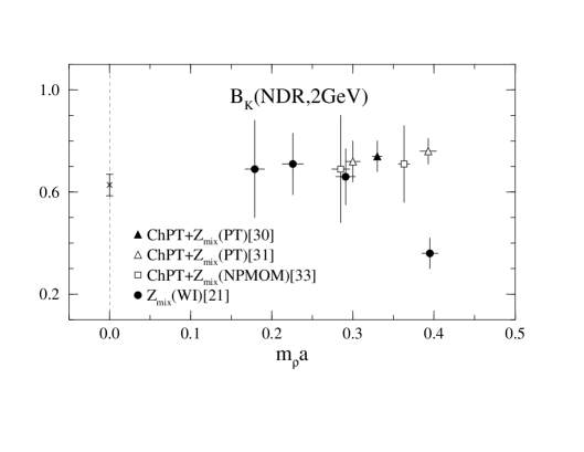
Figure 3: Quenched $B_{K}({\rm NDR,2GeV})$ with the Wilson (filled symbols) and SW (open symbols) quark actions as a function of $m_{\rho}a$. For the KS result in the continuum limit (cross) see Fig. 1.

Figure 4: Mixing coefficients $z_{1},\dots,z_{4}$ obtained with (a) the NPMOM method and (b) the Ward identity method as a function of $p^{2}a^{2}$ around strange quark mass with the Wilson quark action at $\beta=6.3$.

We have two purposes to calculate $B_{K}$ with the Wilson quark action. One is to demonstrate that the Wilson result is consistent with the KS result, which would give confidence to the lattice QCD calculation of $B_{K}$. The other is an application to the heavy-light meson system for which the interpretation of flavor quantum numbers with the KS action is problematic.

While steady progress has been achieved so far with the KS quark action, studies with the Wilson quark action are rather stagnant. This is due to a non-trivial mixing between the weak four-fermi operator ${\cal O}_{LL}={\bar{s}}\gamma_{\mu}(1-\gamma_{5})d\cdot{\bar{s}}\gamma_{\mu}(1-\gamma_{5})d$ and other four-fermi operators with different chiralities. One of the mixing operators is ${\bar{s}}\gamma_{5}d\cdot{\bar{s}}\gamma_{5}d$. Numerical studies show that the magnitude of the matrix element $\langle{\bar{K}}^{0}|{\bar{s}}\gamma_{5}d\cdot{\bar{s}}\gamma_{5}d|K^{0}\rangle$ is a factor of 10 larger than that of $\langle{\bar{K}}^{0}|{\cal O}_{LL}|K^{0}\rangle$ at the point of the physical kaon mass (see, e.g., refs. [30, 21]). This can be reasonably expected from the ratio of their vacuum saturation approximations:

$$\frac{11}{16}\frac{\langle{\bar{K}}^{0}|{\bar{s}}\gamma_{5}d|0\rangle\langle 0|{\bar{s}}\gamma_{5}d|K^{0}\rangle}{\langle{\bar{K}}^{0}|{\bar{s}}\gamma_{\mu}\gamma_{5}d|0\rangle\langle 0|{\bar{s}}\gamma_{\mu}\gamma_{5}d|K^{0}\rangle}-\frac{1}{16}\approx-17$$ (2)

with the aid of the PCAC relation. In this case the mixing problem is not adequately treated with one-loop perturbation theory, because two-loop contributions are potentially large: $|\alpha_{\rm latt}^{2}\langle{\bar{K}}^{0}|{\bar{s}}\gamma_{5}d\cdot{\bar{s}}\gamma_{5}d|K^{0}\rangle/\langle{\bar{K}}^{0}|{\cal O}_{LL}|K^{0}\rangle|\\ \hbox to0.0pt{\lower 3.5pt\hbox{$\mathchar 0\relax\sim$}\hss}\raise 1.0pt\hbox{$>$}0.1$, where we assume $\alpha_{\rm latt}=0.15-0.2$ as the currently accessible strong coupling constant with tadpole improvement. This fact compels us to control the operator mixing non-perturbatively.

Three major non-perturbative methods have been proposed so far. The most conventional method is to rely on chiral perturbation theory[30, 31]. The mixing structure of the weak four-fermi operator is expressed by ${\hat{\cal O}_{LL}}={\cal O}_{LL}+\sum_{i=1}^{4}z_{i}{\cal O}_{i},$ where the mixing operators are arranged into the Fierz eigenbasis given by ${\cal O}_{1}=SS+TT+PP$, ${\cal O}_{2}=SS-TT/3+PP$, ${\cal O}_{3}=VV-AA+2(SS-PP)$ and ${\cal O}_{4}=VV-AA-2(SS-PP)$, with $VV={\bar{s}}\gamma_{\mu}d\cdot{\bar{s}}\gamma_{\mu}d$, $AA={\bar{s}}\gamma_{\mu}\gamma_{5}d\cdot{\bar{s}}\gamma_{\mu}\gamma_{5}d$, $SS={\bar{s}}d\cdot{\bar{s}}d$, $PP={\bar{s}}\gamma_{5}d\cdot{\bar{s}}\gamma_{5}d$ and $TT={\bar{s}}\sigma_{\mu\nu}d\cdot{\bar{s}}\sigma_{\mu\nu}d/2$. The authors of ref. [30] assume the general form of the chiral expansion up to $O(p^{4})$ for the matrix elements of ${\hat{\cal O}_{LL}^{\rm pert}}$: $\langle{\bar{K}}^{0}(p_{f})|{\hat{\cal O}_{LL}^{\rm pert}}|K^{0}(p_{i})\rangle\hfill=\hfill\alpha\hfill+\hfill\beta m_{K}^{2}\hfill+\hfill\gamma p_{i}\cdot p_{f}\\ +\delta_{1}m_{K}^{4}+\delta_{2}m_{K}^{2}p_{i}\cdot p_{f}+\delta_{3}(p_{i}\cdot p_{f})^{2},$ where chiral logarithms are ignored. One-loop perturbative expressions are used for the mixing coefficients $z_{1},\dots,z_{4}$ in ${\hat{\cal O}_{LL}^{\rm pert}}$. The coefficients in the chiral expansion of $\langle{\bar{K}}^{0}(p_{f})|{\hat{\cal O}_{LL}^{\rm pert}}|K^{0}(p_{i})\rangle$ can be determined by changing the quark mass and the spatial momentum of ${\bar{K}}^{0}$ and $K^{0}$, with which we can eliminate pure lattice artifacts of $\alpha$, $\beta$ and $\delta_{1}$ terms. In practical applications of this method, however, it is difficult to fix $\delta_{1}$, $\delta_{2}$ and $\delta_{3}$ with good precision. The results for $B_{K}$ are plotted in Fig. 3(triangles), which seem to be reasonable estimates compared with the KS result at the continuum limit. Nonetheless, this method is not promising for controlling systematic errors, since it contains unknown uncertainties from higher order effects of ChPT which survive even in the continuum limit. Another defect of this method is that it cannot be applied to the heavy-light meson system.

The second method is to determine the mixing coefficients $z_{1},\dots,z_{4}$ using the NPMOM method[23]. We require the Fourier transformed vertex function should be proportional to the tree-level Dirac structure: $G_{s}^{-1}(p)G_{s}^{-1}(p)\\ \langle{\hat{\cal O}}_{LL}[ss{\bar{d}}{\bar{d}}](p)\rangle G_{\bar{d}}^{-1}(p)G_{\bar{d}}^{-1}(p)\hfill\propto\hfill\gamma_{\mu}(1\hfill-\hfill\gamma_{5})\\ \otimes\gamma_{\mu}(1-\gamma_{5}),$ where $[ss{\bar{d}}{\bar{d}}](p)$ represents $s(p)s(p){\bar{d}}(p){\bar{d}}(p)$. $G_{s,{\bar{d}}}(p)$ denote the free quark propagators with off-shell quark momentum $p$. In Fig. 4(a) we plot the mixing coefficients $z_{1},\dots,z_{4}$ as a function of $p^{2}a^{2}$, where the vertical line corresponds to about 2GeV. As mentioned in the previous subsection, this method can work under the condition $\Lambda_{\rm QCD}\ll p\ll a^{-1}$. A strong $p$ dependence of $z_{1},\dots,z_{4}$ below $p\approx 2$GeV indicates that non-perturbative contamination plagues the mixing coefficients up to around 2GeV. The Gribov uncertainty in Landau gauge fixing is another source of systematic errors.

In the third method the mixing coefficients $z_{1},\dots,z_{4}$ are determined to satisfy the continuum Ward identity up to $O(a)$ for the external off-shell quarks with momentum $p$[21, 32]: $\langle\nabla_{\mu}A_{\mu}{\hat{\cal O}}_{LL}[ss{\bar{d}}{\bar{d}}](p)\rangle=2m_{q}\langle P{\hat{\cal O}_{LL}}[ss{\bar{d}}{\bar{d}}](p)\rangle+\langle i\delta_{A}\{{\hat{\cal O}_{LL}}[ss{\bar{d}}{\bar{d}}](p)\}\rangle+O(a).$ It should be stressed that this method can fix the mixing coefficients without $O(m_{q})$ ambiguities for the $(27,1)$-operator in the flavor SU(3)${}_{L}\times$SU(3)_R representation which is relevant to $B_{K}$ and $K\rightarrow\pi\pi[I=2]$ amplitude, while some ambiguities of $O(m_{q})$ remain in the case of the $(8,1)$-operator associated with $K\rightarrow\pi\pi[I=0]$ decay[32]. Figure 4(b) shows the momentum dependence of the mixing coefficients. The Ward identity method requires the condition $p\ll a^{-1}$ to avoid the cut-off effects. We observe only weak dependence over a wide range $p^{2}a^{2}\hbox to0.0pt{\lower 3.5pt\hbox{$\mathchar 0\relax\sim$}\hss}\raise 1.0pt\hbox{$<$}1.0$, which contrasts to the NPMOM results in Fig. 4(a). In principle, however, both results are expected to be consistent at the limit of large external quark momentum[23]. The Gribov uncertainties in this method could be avoided by employing the Schrödinger functional technique.

In Fig. 3 we summarize recent quenched results for $B_{K}$ with the Wilson and SW quark actions. It is encouraging to be able to deal with the mixing problem without ChPT; still, large errors hinder the direct comparison with the KS result in the continuum limit.

3 $K\rightarrow\pi\pi$ decay amplitudes

There are two major difficulties in the lattice QCD calculation of $K\rightarrow\pi\pi$ decay amplitudes. The first one is the phase shift in $\pi$-$\pi$ final state interactions, which cannot be directly calculated with real Green functions on a Euclidean lattice[34]. Secondly, we have to control the operator mixing. For the Wilson quark action we have ${\cal O}_{\pm}^{\rm cont}=z_{\pm}{\cal O}_{\pm}^{\rm latt}+z_{\pm}^{\prime}{\cal O}_{\pm}^{\prime}+(m_{c}-m_{u})\{z_{3}{\bar{s}}d+z_{3}^{\prime}(m_{s}-m_{d}){\bar{s}}\gamma_{5}d+z_{5}g_{0}{\bar{s}}\sigma_{\mu\nu}F_{\mu\nu}d\},$ where ${\cal O}_{\pm}^{\prime}$ are dimension-six operators arising from the explicit chiral symmetry breaking in the action. The mixing with ${\bar{s}}d$, ${\bar{s}}\gamma_{5}d$ and $g_{0}{\bar{s}}\sigma_{\mu\nu}F_{\mu\nu}d$ is generated by the “eye” diagram, in which two quarks in ${\cal O}_{\pm}$ generate a quark loop by contracting with each other. The factors $(m_{c}-m_{u})$ and $(m_{s}-m_{d})$ are required by GIM mechanism and CPS symmetry[35] respectively.

The simplest solution to overcome these difficulties is calculating the amplitude $\langle\pi({\vec{p}}=0)\pi({\vec{p}}=0)|{\cal O}_{\pm}^{\rm cont}|K({\vec{p}}_{K}=0)\rangle$ with $m_{s}=m_{d}$[36]. The final state pions at rest relative to each other generate no phase shift; the operator mixing is completely avoided by CPS symmetry and parity conservation. This method, however, requires ChPT to convert the amplitudes with the unphysical condition to those with the physical one. The next simplest method may be evaluation of the $K\rightarrow\pi$ matrix elements with the KS quark action[35, 37]. Although the mixing with ${\cal O}_{\pm}^{\prime}$ can be avoided by the $\rm U_{A}(1)$ chiral symmetry retained in the action, subtraction of the lower dimensional operator is still necessary. This method also has to rely on ChPT. A new idea to avoid the operator mixing problem was recently proposed[38], which is an attempt to directly calculate the hadronic matrix element of the $T$-product of weak currents $T[J_{\mu L}(x)J^{\dagger}_{\mu L}(0)]$ in the region $a\ll|x|\ll\Lambda_{\rm QCD}^{-1}$. However, its practical feasibility is questionable even with 1 Teraflops machine because of the requirement of large cut-off.

In recent years Golterman and his collaborators[4, 5] have studied the $K\rightarrow\pi\pi$ decay amplitudes using ChPT and the quenched formulation of ChPT(QChPT)[39] up to one-loop level, which enable us to investigate three systematic effects contaminating the lattice QCD calculation: unphysical kinematics, finite volume effects, and quenching. Only the first one can be estimated at the tree level. Although an $O(m_{K}^{2}/\Lambda_{\chi}^{2})$ uncertainty still remains in this calculation due to the unavailability of the $O(p^{4})$ low-energy constant terms, we should note two points: First, finite volume effects can arise only from the loop diagrams. Second, we can investigate the difference of the chiral properties between full QCD and quenched QCD, which emerge at the one-loop level.

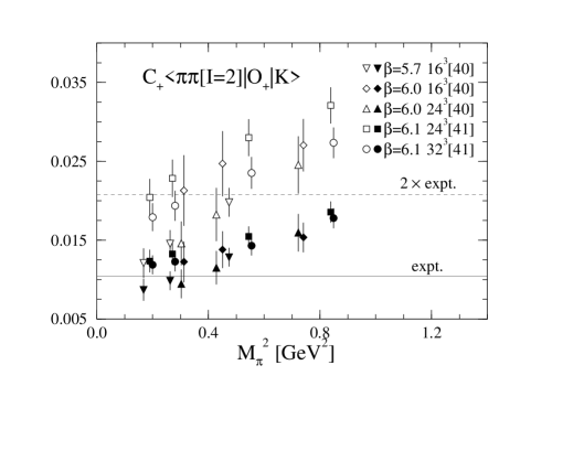
Figure 5: $K\rightarrow\pi\pi$ decay amplitude in $\Delta I=3/2$ channel with (filled symbols) and without (open symbols) one-loop corrections of QChPT. Data are plotted as a function of lattice meson mass.

In Fig. 5 we plot the physical $K\rightarrow\pi\pi[I=2]$ amplitude as a function of the degenerate $K$ and $\pi$ meson mass on the quenched lattice. They are obtained from the matrix element $\langle\pi({\vec{p}}=0)\pi({\vec{p}}=0)|{\cal O}_{+}^{\rm cont}|K({\vec{p}}_{K}=0)\rangle$ calculated with the Wilson quark action[40, 41], where ${\cal O}_{+}^{\rm cont}$ is renormalized in NDR scheme at the scale 2GeV employing the tadpole improvement. The conversion to the physical matrix element is made by

$$\langle\pi\pi|{\cal O}_{+}|K\rangle_{\rm phys}=\frac{m_{K}^{2}-m_{\pi}^{2}}{2M_{\pi}^{2}}\cdot Y\cdot\langle\pi\pi|{\cal O}_{+}|K\rangle_{\rm latt},$$ (3)

where the factor $Y$ denotes the one-loop contribution given by

$$Y=\frac{1+\frac{m_{\pi}^{2}}{(4\pi f_{\pi})^{2}}[-104.73-29.57{\rm log}\left(\frac{m_{\pi}}{\Lambda}\right)^{2}]}{1+\frac{M_{\pi}^{2}}{(4\pi F_{\pi})^{2}}[-3{\rm log}\left(\frac{M_{\pi}}{\Lambda}\right)^{2}+F(M_{\pi}L)]}.$$ (4)

$F(M_{\pi}L)$ represents finite size effects, whose expression is $F(M_{\pi}L)=17.827/(M_{\pi}L)+12\pi^{2}/(M_{\pi}L)^{3}$. The tree-level results(open symbols), which are obtained by setting $m_{\pi}=136$MeV, $m_{K}=497$MeV and $Y=1$ in eq.(3), are about two times larger than the experimental value. However, once we include the one-loop effects with $Y$ of eq.(4) employing $f_{\pi}=F_{\pi}=132$MeV and $\Lambda=1$GeV, the lattice results are reduced and are much closer to the experimental value. The one-loop corrections are rather substantial. For example, the corrections are $-40\%$ for unphysical kinematics, $-30\%$ for finite volume effects, and $+30\%$ for quenching around $M_{\pi}\approx m_{K}$ at $\beta=6.1$ with the $24^{3}$ spatial volume(squares). It is also noted that the size dependence observed in the tree-level results is almost explained through the one-loop calculation.

For the $\Delta I=1/2$ amplitude, the one-loop calculation with QChPT[5] finds that the quenched matrix element $\langle\pi({\vec{p}}=0)\pi({\vec{p}}=0)|{\cal O}_{\pm}^{\rm cont}|K({\vec{p}}_{K}=0)\rangle$ has finite volume contributions in proportion to $M_{\pi}L$, which arise from the rescattering diagram of the two pions. Although this fact could jeopardize the numerical calculation of $\langle\pi({\vec{p}}=0)\pi({\vec{p}}=0)|{\cal O}_{\pm}^{\rm cont}|K({\vec{p}}_{K}=0)\rangle$ in the quenched approximation, fortunately, we have had no work so far. This dangerous finite size effect caused by the $\pi$-$\pi$ interactions can be avoided by employing the $K\rightarrow\pi$ matrix element. Its numerical calculation was tried by the OSU group employing the KS quark action[42]. Although their result shows a consistency with the experimental value around $a^{-1}\approx 2.8$GeV, it is not convincing because of their use of the tree-level ChPT and the statistical error of $40\%$.

4 Proton decay amplitudes

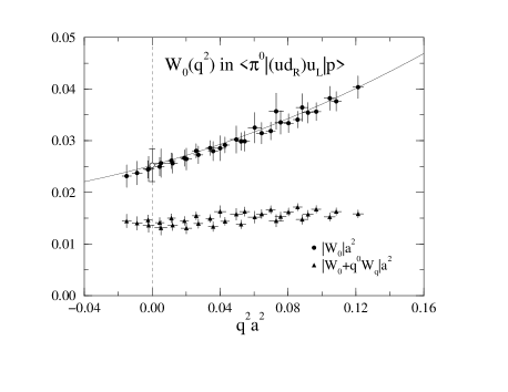
Figure 6: $q^{2}a^{2}$ dependence of the relevant form factor (circles) in $\langle\pi^{0}|(ud_{R})u_{L}|p\rangle$, together with the form factor (triangles) employed in ref. [8] for comparison. Solid line denotes the fitting result.

One of the most important features of the study of the baryon number violating processes is that the low energy effective theory is described in terms of SU(3)$\times$SU(2)$\times$U(1) symmetry, which enables us to make a model independent analysis. All dimension-six operators associated with baryon number violating processes are classified in the four types under the requirement of SU(3)$\times$SU(2)$\times$U(1) invariance [43, 44]. In the two-component notation of ref. [44] they are given by ${\cal O}^{(1)}_{abcd}=(d^{\alpha}_{aR}u^{\beta}_{bR})(q^{\gamma}_{icL}l_{jdL})\epsilon_{\alpha\beta\gamma}\epsilon_{ij}$, ${\cal O}^{(2)}_{abcd}=(q^{\alpha}_{iaL}q^{\beta}_{jbL})(u^{\gamma}_{cR}l_{dR})\epsilon_{\alpha\beta\gamma}\epsilon_{ij}$, ${\cal O}^{(3)}_{abcd}=(q^{\alpha}_{iaL}q^{\beta}_{jbL})(q^{\gamma}_{kcL}l_{ndL})\epsilon_{\alpha\beta\gamma}\epsilon_{in}\epsilon_{jk}$ and ${\cal O}^{(4)}_{abcd}=(d^{\alpha}_{aR}u^{\beta}_{bR})(u^{\gamma}_{cR}l_{dR})\epsilon_{\alpha\beta\gamma}$, where $\alpha$,$\beta$,$\gamma$ are SU(3) color indices, $i$,$j$,$k$,$n$ are SU(2) indices, $a$,$b$,$c$,$d$ are generation indices and $L$ and $R$ denote left- and right-handed fields. Specifying the decay processes of interest, in our case (proton,neutron)$\rightarrow$($\pi$,$K$) +($\bar{\nu}$, $e^{+}$, $\mu^{+}$), we can list the complete set of independent matrix elements in QCD with the assumption of isospin symmetry: $\langle\pi^{0}|\epsilon_{\alpha\beta\gamma}(u^{\alpha}d^{\beta}_{R,L})u^{\gamma}_{L}|p\rangle$, $\langle\pi^{+}|\epsilon_{\alpha\beta\gamma}(u^{\alpha}d^{\beta}_{R,L})d^{\gamma}_{L}|p\rangle$, $\langle K^{0}|\epsilon_{\alpha\beta\gamma}(u^{\alpha}s^{\beta}_{R,L})u^{\gamma}_{L}|p\rangle$, $\langle K^{+}|\epsilon_{\alpha\beta\gamma}(u^{\alpha}d^{\beta}_{R,L})s^{\gamma}_{L}|p\rangle$, $\langle K^{+}|\epsilon_{\alpha\beta\gamma}(u^{\alpha}s^{\beta}_{R,L})d^{\gamma}_{L}|p\rangle$ and $\langle K^{+}|\epsilon_{\alpha\beta\gamma}(d^{\alpha}s^{\beta}_{R,L})u^{\gamma}_{L}|p\rangle$. All we have to calculate in lattice QCD are these matrix elements.

Under the requirement of Lorentz invariance, we find that the matrix elements of ${\cal O}^{{{B}{/}}}$ between the nucleon($N$) and the pseudoscalar(PS) meson can have two form factors:

$$\langle PS(\vec{p})|{\cal O}^{{{B}{/}}}_{L}|N^{s}(\vec{k})\rangle=P_{L}(W_{0}(q^{2})+W_{q}(q^{2}){{{q}{/}}})u^{s},$$ (5)

where $u^{s}$ denotes the Dirac spinor with spin state $s$. In the lattice calculation, $\vec{k}=\vec{0}$ is chosen for the nucleon spatial momentum and $\vec{p}=\vec{k}-\vec{q}\neq\vec{0}$ for the PS meson. Although the $W_{q}$ term in eq.(5) is irrelevant in the physical decay amplitude, because its contribution is $O(m_{l})$ after the multiplication of anti-lepton spinor, we have to disentangle these two form factors in the lattice QCD calculation. As pointed out by JLQCD[10], the previous papers[8, 9] gave wrong results without realizing the existence of $W_{q}$ term: they eventually evaluated $W_{0}+q^{0}W_{q}$ instead of $W_{0}$.

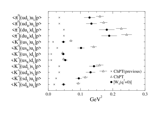
Figure 7: Comparison of relevant form factors (circle) with predictions of tree-level ChPT (triangles). For the previous ChPT results (crosses) see text.

In Fig. 6 the quenched results for $W_{0}(q^{2})$ in $\langle\pi^{0}|(ud_{R})u_{L}|p\rangle$ calculated by JLQCD[10] with the Wilson quark action at $\beta=6.0$ are compared with $W_{0}+q^{0}W_{q}$ obtained by following the method in ref. [8]. The magnitude of $W_{0}(q^{2})$ is more than two times larger than that of $W_{0}+q^{0}W_{q}$. The value at $q^{2}=0$(open circle) is obtained by fitting the data with the function of $c_{0}+c_{1}q^{2}+c_{2}q^{4}+c_{3}m_{ud}+c_{4}m_{s}$. In Fig. 7 we compare the results obtained by the direct method(circles) with those by the indirect one(triangles) using tree-level ChPT, where the so-called $\alpha,\beta$ parameters are $|\alpha|=0.015(1){\rm GeV}^{3}$ and $|\beta|=0.014(1){\rm GeV}^{3}$. We observe that both results are roughly comparable, which could leads to the conclusion that the large discrepancy between two methods found in refs.[8, 9] is mainly due to the neglect of the $W_{q}(q^{2})$ term in eq.(5). Another important point in Fig. 7 is that the JLQCD results are much larger than the tree-level ChPT predictions with $|\alpha|=|\beta|=0.003$GeV³(crosses), which is the smallest value among various model estimations.

5 Domain wall QCD

If we can make the length of the fifth dimension $N$ sufficiently large in the practical implementation of the domain wall QCD on the lattice, the desirable features would emerge as: (i) no fine tuning for the chiral limit up to $O(1/a{\rm e}^{-\alpha N})$, (ii) $O(a^{2})$ scaling violation up to $O(a{\rm e}^{-\alpha^{\prime}N})$ and (iii) no mixing for four-fermi operators up to $O(g^{2}{\rm e}^{-\alpha^{\prime\prime}N})$. The flavor symmetry is retained at any number $N$. The KS quark action, however, can realize the above features without corrections except the flavor symmetry. The cost of numerical studies with the domain wall quark are the fifth dimension with the extension $N$ and choosing the optimal value for the domain wall height $M$. The RIKEN-BNL-Columbia group presented numerical studies for weak matrix elements relevant to ${\bar{K}}^{0}$-$K^{0}$ mixing, $K\rightarrow\pi\pi$ decays and the prediction of $\epsilon^{\prime}/\epsilon$[24], assuming the naive chiral properties realized at the infinite $N$[24]. In Fig. 1 we already plotted the quenched results for $B_{K}$ by the RIKEN-BNL-Columbia group. Their results are considerably smaller than the KS results at finite lattice spacings, and the discrepancy is likely to survive even in the continuum limit. At present it is not clear what causes this difference.

Perturbative calculation in domain wall QCD, which was initiated in ref.[45], has been applied to evaluation of the renormalization factors for the quark mass[46, 47] and the bilinear operators[46] consisting of four-dimensional quarks which were referred to as $q(x)$ in ref. [12]. The Tsukuba group[46] shows that $Z_{S}=Z_{P}=Z_{m}^{-1}$ and $Z_{V}=Z_{A}$ at $N\rightarrow\infty$, which is expected when the chiral Ward-Takahashi identity hold exactly. The peculiar feature in the renormalization of the domain wall QCD is an appearance of the overlap factor $(1-|1-M|^{2})Z_{w}$ for the four-dimensional quark fields. The one-loop coefficient of $Z_{w}$ is of $O(10-10^{2})$ for $|1-M|\hbox to0.0pt{\lower 3.5pt\hbox{$\mathchar 0\relax\sim$}\hss}\raise 1.0pt\hbox{$>$}0.1$ without mean-field improvement. This could be dangerous because current numerical studies employ $M\hbox to0.0pt{\lower 3.5pt\hbox{$\mathchar 0\relax\sim$}\hss}\raise 1.0pt\hbox{$>$}1.6$[24]. In the mean-field analysis, however, they find that $M$ should be replaced by ${\tilde{M}}=M+4(u-1)$, where $u^{4}$ corresponds to the expectation value of the plaquette, and the magnitude of the one-loop coefficient for $Z_{w}$ is reduced to $O(1)$ for $|1-{\tilde{M}}|\hbox to0.0pt{\lower 3.5pt\hbox{$\mathchar 0\relax\sim$}\hss}\raise 1.0pt\hbox{$<$}0.8$. This fact suggests that the mean field improvement is indispensable for the perturbative renormalization factors in domain wall QCD. The $\rho$ meson decay constant $f_{\rho}$ obtained with $V^{q}={\bar{q}}(x)\gamma_{\mu}q(x)$ and with the five-dimensional conserved current $V^{\rm con}$ gives a testing ground for the validity of perturbation theory[48]. Both results at $\beta=6.0$ are compared in Fig. 8(a). They show a consistency within error bars once the perturbative corrections are applied to $V^{q}$. We also observe a similar situation for the case of the pion decay constant in Fig. 8(b). This is an encouraging result; still, the scaling violation effects should be checked. The Tsukuba group also calculated the renormalization factors for the three- and four-quark operators associated with proton decay and weak interactions[49]. They find that the operators in domain wall QCD at infinite $N$ can be renormalized without any operator mixing between different chiralities, as opposed to the Wilson case.

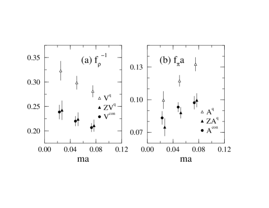
Figure 8: $f_{\rho}^{-1}$ and $f_{\pi}$ obtained from the five-dimensional conserved current (circles) and the four-dimensional local current with (filled triangles) and without (open triangles) perturbative renormalization factors.

The good chiral properties of the four-dimensional quarks in domain wall QCD observed in the numerical simulations and the perturbative calculations can be understood from the point of view of the exact chiral symmetry based on the Ginsparg-Wilson relation. The partition function of domain wall fermion with the subtraction of the Pauli-Villars field at finite $N$ can be written as a determinant of the truncated overlap Dirac operator $D_{N}$[50] which satisfies the Ginsparg-Wilson relation in the limit of infinite $N$. The authors of ref. [51] find that the effective Dirac operator $D_{N}^{\rm eff}$ for the four-dimensional quarks in domain wall QCD with finite $N$, which is obtained by integrating out the $N-1$ heavy fermion fields, is related to $D_{N}$: ${D_{N}^{\rm eff}}^{-1}(x,y)+\delta(x,y)={D_{N}}^{-1}(x,y)$. With the use of this relation they show that the Green functions consisting of $q(x)$ and ${\bar{q}}(x)$ in domain wall QCD with finite $N$ can be related to those consisting of the fermion fields described by the truncated overlap Dirac operator.

6 Conclusions

The sizable magnitude of the $O(\alpha^{2})$ uncertainties found in the systematic study of $B_{K}$ with the KS quark action makes manifest the necessity of using the non-perturbative renormalization method. The essential problem in the non-perturbative renormalization of QCD, which is the question how to relate the high-energy perturbative regime to the low-energy hadronic scale, is overcome by the Schrödinger functional method. For the Wilson $B_{K}$ the operator mixing problem is now managed non-perturbatively without the use of any effective theories; while we still need to reduce statistical errors.

In $K\rightarrow\pi\pi$ studies one-loop corrections in QChPT can almost explain the discrepancy between quenched lattice results and the experimental value for the $\Delta I=3/2$ transition.

Essential progress has been made in evaluating the proton decay amplitudes. The first correct calculation shows that the values of the amplitudes are comparable with the tree-level ChPT predictions.

The application of the domain wall quark formulation to the calculation of the weak matrix elements is a fascinating issue. Pilot numerical studies have been pursued and perturbative renormalization factors for the relevant operators are now available.

7 Acknowledgments

I would like to thank S. Aoki, C. Bernard, T. Blum, M. Golterman, N. Ishizuka, T. Izubuchi, Y. Kikukawa, E. Pallante, Y. Taniguchi, N. Tsutsui, R. Sommer, A. Soni and P. Weisz for communicating their results and for discussions. I would also like to thank C. Bernard and M. Golterman for comments on the manuscript. This work is supported in part by a JSPS Fellowship.

References

- [1] G. Kilcup et al., Phys. Rev. Lett. 64 (1990) 25; N. Ishizuka et al., ibid. 71 (1993) 24.
- [2] JLQCD Collab., S. Aoki et al., Phys. Rev. Lett. 80 (1998) 5271.
- [3] See, e.g., C. Bernard and A. Soni, Nucl. Phys. B (Proc. Suppl.) 9 (1989) 155.
- [4] M. Golterman and K.-C. Leung, Phys. Rev. D56 (1997) 2950.
- [5] M. Golterman and E. Pallante, this volume.
- [6] Y. Hara et al., Phys. Rev. D34 (1986) 3399.
- [7] K. Bowler et al., Nucl. Phys. B296 (1988) 431.
- [8] M. Gavela et al., Nucl. Phys. B312 (1989) 269.
- [9] JLQCD Collab., N. Tsutsui et al., Nucl. Phys. B (Proc. Suppl.) 73 (1999) 297.
- [10] JLQCD Collab. (presented by N. Tsutsui), this volume.
- [11] Y. Shamir, Nucl. Phys. B406 (1993) 90.
- [12] V. Furman and Y. Shamir, Nucl. Phys. B439 (1995) 54.
- [13] T. Blum and A. Soni, Phys. Rev. D56 (1997) 174; Phys. Rev. Lett. 79 (1997) 3595.
- [14] R. Petronzio, this volume.
- [15] S. Sharpe, Nucl. Phys. B (Proc. Suppl.) 34 (1994) 403.
- [16] G. Kilcup et al., Nucl. Phys. B (Proc. Suppl.) 53 (1997) 345.
- [17] S. Sharpe, in Proc. of the 1994 TASI School, ed. J. Donoghue (World Scientific, Singapore 1995).
- [18] CPPACS Collab. (presented by R. Burkhalter and T. Kaneko), this volume.
- [19] G. Martinelli et al., Nucl. Phys. B445 (1995) 81.
- [20] M. Göckeler et al., Nucl. Phys. B544 (1999) 699.
- [21] JLQCD Collab., S. Aoki et al., Phys. Rev. Lett. 81 (1998) 1778; Phys. Rev. D60 (1999) 034511.
- [22] JLQCD Collab., S. Aoki et al., Phys. Rev. Lett. 82 (1999) 4392.
- [23] A. Donini et al., Eur. Phys. J. C10 (1999) 121.
- [24] RIKEN-BNL-Columbia Collab. (presented by T. Blum, C. Dawson and A. Soni), this volume.
- [25] K. Jansen et al., Phys. Lett. B372 (1996) 275.
- [26] S. Sint, Nucl. Phys. B421 (1994) 135; ibid. B451 (1995) 416.
- [27] ALPHA Collab., S. Capitani et al., Nucl. Phys. B544 (1999) 669.
- [28] K. Jansen, this volume.
- [29] M. Kurth, this volume.
- [30] R. Gupta, T. Bhattacharya and S. Sharpe, Phys. Rev. D55 (1997) 4036.
- [31] UKQCD Collab., L. Lellouch et al., Nucl. Phys. B (Proc. Suppl.) 73 (1999) 312.
- [32] M. Bochicchio et al., Nucl. Phys. B262 (1985) 331; L. Maiani et al., ibid. B289 (1987) 505.
- [33] C. Allton et al., Phys. Lett. B453 (1999) 30.
- [34] L. Maiani and M. Testa, Phys. Lett. B245 (1990) 585.
- [35] C. Bernard et al., Phys. Rev. D32 (1985) 2343.
- [36] C. Bernard et al., Nucl. Phys. B (Proc. Suppl.) 4 (1988) 483.
- [37] G. Kilcup and S. Sharpe, Nucl. Phys. B283 (1987) 493; S. Sharpe et al., ibid. B286 (1987) 253.
- [38] C. Dawson et al., Nucl. Phys. B514 (1998) 313.
- [39] S. Sharpe, Phys. Rev. D46 (1992) 3146. C. Bernard and M. Golterman, ibid. D46 (1992) 853.
- [40] C. Bernard, in Proc. of the 1989 TASI School, eds. T. DeGrand and D. Toussaint (World Scientific, Singapore, 1990).
- [41] JLQCD Collab., S. Aoki et al., Phys. Rev. D58 (1998) 054503.
- [42] D. Pekurovsky and G. Kilcup, hep-lat /9812019.
- [43] S. Weinberg, Phys. Rev. Lett. 43 (1979) 1566; F. Wilczek and A. Zee, ibid. 43 (1979) 1571.
- [44] L. Abbott and M. Wise, Phys. Rev. D22 (1980) 2208.
- [45] S. Aoki and Y. Taniguchi, Phys. Rev. D59 (1999) 054510.
- [46] S. Aoki et al., Phys. Rev. D59 (1999) 094505.
- [47] T. Blum, A. Soni and M. Wingate, hep-lat/9902016
- [48] T. Izubuchi, this volume.
- [49] S. Aoki et al., hep-lat/9902008
- [50] H. Neuberger, Phys. Rev. D57 (1998) 5417.
- [51] Y. Kikukawa and T. Noguchi, hep-lat /9902022.