Scalar Quarkonium Masses and Mixing with the Lightest Scalar Glueball

Abstract

We evaluate the continuum limit of the valence (quenched) approximation to the mass of the lightest scalar quarkonium state for a range of different quark masses and to the mixing energy between these states and the lightest scalar glueball. Our results support the interpretation of $f_{0}(1710)$ as composed mainly of the lightest scalar glueball.

I Introduction

Evidence that $f_{0}(1710)$ is composed mainly of the lightest scalar glueball is now given by two different sets of numerical determinations of QCD predictions using the theory’s lattice formulation in the valence (quenched) approximation. A calculation on GF11 [2] of the width for the lightest scalar glueball to decay to all possible pseudoscalar pairs, on a $16^{3}\times 24$ lattice with $\beta$ of 5.7, corresponding to a lattice spacing $a$ of 0.140(4) fm, gives 108(29) MeV. This number combined with any reasonable guesses for the effect of finite lattice spacing, finite lattice volume, and the remaining width to multibody states yields a total width small enough for the lightest scalar glueball to be seen easily in experiment. For the infinite volume continuum limit of the lightest scalar glueball mass, a reanalysis [3] of a calculation on GF11 [4], using 25000 to 30000 gauge configurations, gives 1648(58) MeV. An independent calculation by the UKQCD-Wuppertal [5] collaboration, using 1000 to 3000 gauge configurations, when extrapolated to the continuum limit according to Refs. [3, 6] yields 1567(88) MeV. A more recent calculation using an improved action [7] gives 1730(94) MeV. The three results combined become 1656(47) MeV. A phenomenological model of the glueball spectrum which supports this prediction is discussed in Ref. [8].

Among established resonances with the quantum numbers to be a scalar glueball, all are clearly inconsistent with the mass calculations except $f_{0}(1710)$ and $f_{0}(1500)$. Between these two, $f_{0}(1710)$ is favored by the mass result with largest statistics, by the combined result, and by the expectation [9] that the valence approximation will lead to an underestimate of the scalar glueball’s mass. Refs. [2, 9] interpret $f_{0}(1500)$ as dominantly composed of strange-antistrange, $s\overline{s}$, scalar quarkonium. A possible objection to this interpretation, however, is that $f_{0}(1500)$ apparently does not decay mainly to states containing an $s$ and an $\overline{s}$ quark [10]. In part for this reason, Ref. [11] interprets $f_{0}(1500)$ as composed mainly of the lightest scalar glueball and $f_{0}(1710)$ as largely $s\overline{s}$ scalar quarkonium. A second objection is that while the Hamiltonian of full QCD couples quarkonium and glueballs, so that physical states should be linear combinations of both, mixing is not treated quantitatively in Ref. [2]. In the extreme, mixing could lead to $f_{0}(1710)$ and $f_{0}(1500)$ each half glueball and half quarkonium.

Using the valence approximation for a fixed lattice period $L$ of about 1.6 fm and a range of different values of quark mass, we have now calculated the continuum limit of the mass of the lightest scalar $q\overline{q}$ states and the continuum limit of the mixing energy between these states and the lightest scalar glueball. Our calculations have been done with four different choices of lattice spacing. Continuum predictions are found by extrapolation of results obtained from the three smallest values of lattice spacing. For the two choices of lattice spacing we have also calculated scalar $q\overline{q}$ masses on lattices with $L$ of about 2.3 fm, and for one choice of lattice spacing we have found scalar quarkonium-glueball mixing energies on a lattice with $L$ of about 2.3 fm. Preliminary versions of this work are reported in Refs. [9, 12, 13].

Our results provide answers to the objections to the interpretation of $f_{0}(1710)$ as largely the lightest scalar glueball. For the valence approximation to the infinite volume continuum limit of the $s\overline{s}$ scalar mass we find a value significantly below the valence approximation scalar glueball mass. This prediction makes improbable, in our opinion, the identification [11] of $f_{0}(1500)$ as primarily a glueball and $f_{0}(1710)$ as primarily $s\overline{s}$ quarkonium. Our calculation of glueball-quarkonium mixing energy, combined with the simplification of considering mixing only among the lightest discrete isosinglet scalar states, then yields a mixed $f_{0}(1710)$ which is 73.8(9.5)% glueball and a mixed $f_{0}(1500)$ which is 98.4(1.4)% quarkonium, mainly $s\overline{s}$. The glueball amplitude which leaks from $f_{0}(1710)$ goes almost entirely to the state $f_{0}(1390)$, which remains mainly $n\overline{n}$, normal-antinormal, the abbreviation we adopt for $(u\overline{u}+d\overline{d})/\sqrt{2}$. We find also that $f_{0}(1500)$ acquires an $n\overline{n}$ amplitude with sign opposite to its $s\overline{s}$ component suppressing, by interference, the state’s decay to $K\overline{K}$ final states. Assuming SU(3) flavor symmetry before mixing for the decay couplings of scalar quarkonium to pairs of pseudoscalars, the $K\overline{K}$ decay rate of $f_{0}(1500)$ is suppressed by a factor of 0.39(16) in comparison to the rate of an unmixed $s\overline{s}$ scalar. This suppression is consistent, within uncertainties, with the experimentally observed suppression.

It perhaps is useful to discuss briefly at this point a proposed calculation of mixing between valence approximation quarkonium and glueball states through common decay channels [14] which forms the basis for additional objections to the identification of $f_{0}(1710)$ as primarily a glueball. A detailed examination of problems with the calculation of Ref. [14] appears in Ref. [15]. One defect of the work in Ref. [14] is the omission of quarkonium to glueball transitions by direct annihilation of the quarkonium’s quark and antiquark into chromoelectric field. Direct annihilation is the leading valence approximation contribution to mixing and is evaluated in the present paper. On the other hand, the transitions through two-pseudoscalar intermediate states which Ref. [14] considers include an extra closed quark loop in addition to the quark paths of the direct quark-antiquark annihilation process. Thus according to a systematic scheme for evaluating all quark loop corrections to the valence approximation [15], the decay channel mixing calculation is part of the one-quark-loop correction to the direct annihilation mixing amplitude. As shown in detail in Ref. [15], however, the corrections to the direct annihilation amplitude must include also a counterterm proportional to the pure gauge action. This counterterm is required to compensate for the shift between the screened effective gauge coupling used in the valence approximation and the unscreened bare coupling of full QCD. The counterterm is entirely absent from the calculation of Ref. [14]. As a consequence of this omission and of the omission of the direct quark-antiquark annihilation term, we believe the mixing calculation of Ref. [14] is not correct.

The remainder of this paper is organized as follows. In Section II we describe the Monte Carlo ensembles of gauge field configurations we use. In Section III we present the calculation of scalar quarkonium masses. In Section IV we describe a glueball mass calculation. In Section V we present a calculation of quarkonium-glueball mixing energy. In Section VI we consider the physical mixed glueball and quarkonium states. Finally, Section VII briefly examines consequences of quarkonium-glueball mixing for glueball decay.

II Monte Carlo Ensembles

Our calculations, using Wilson fermions and the plaquette action, were done for four choices of $\beta$ with two different lattice sizes at each of the two smallest $\beta$ giving a total of six combinations of $\beta$ and lattice structure. These are listed in Table I. For each combination of $\beta$ and lattice structure, calculations were typically done with five different choices of $\kappa$. These are listed in Table II along with the corresponding Monte Carlo ensemble sizes. In all cases, a sufficient number of updating sweeps was skipped between successive Monte Carlo configuration to leave no statistically significant correlations between successive pairs. The ensemble of 599 configurations used for two hopping constant choices at $\beta$ of 6.4 is a subset of the 1003 configuration ensemble used for the three other $\kappa$ at $\beta$ of 6.4. At $\beta$ of 5.70 on a lattice $16^{3}\times 24$, the 3870 member ensemble at $\kappa$ of 0.1600 is a subset of the 12186 member ensemble at $\kappa$ of 0.1650, which has no overlap with the 1972 member ensemble used at $\kappa$ of 0.1625 and 0.1650. For all other entries in Table II, all $\kappa$ values share a single ensemble of gauge field configurations.

From the smallest to largest $\beta$, the lattice spacing varies by nearly a factor of 2.7. The smaller lattices with $\beta$ of 5.70 and 5.93, and the lattices with $\beta$ of 6.17 and 6.40 have nearly the same periods in the two (or three) equal space directions and thereby permit extrapolations to zero lattice spacing with nearly constant physical volume.

The values of lattice spacing and lattice period in Table I and conversions from lattice to physical units in the remainder of this article, are determined [3, 4] from the exact solution to the two-loop zero-flavor Callan-Symanzik equation for $\Lambda^{(0)}_{\overline{MS}}a$ with $\Lambda^{(0)}_{\overline{MS}}$ of 234.9(6.2) MeV determined from the continuum limit of $(\Lambda^{(0)}_{\overline{MS}}a)/(m_{\rho}a)$ in Ref. [16]. For $\beta$ from 5.70 to 6.17, the ratio $(\Lambda^{(0)}_{\overline{MS}}a)/(m_{\rho}a)$ in Ref. [16] was found to be constant within statistical errors, thus our results are, within errors, almost certainly the same as those we would have obtained by converting to physical units using values of $m_{\rho}a$. We chose to convert using $\Lambda^{(0)}_{\overline{MS}}a$, however, since Ref. [16] did not find $m_{\rho}a$ at $\beta$ of 6.40, which would be needed for our present calculations.

III Quarkonium Masses

For each ensemble of gauge fields, with two exceptions at $\beta$ of 5.70, we evaluated correlation functions using smeared Coulomb gauge quark and antiquark fields incorporating random sources following Ref. [13]. From these fields we constructed pseudoscalar and scalar quarkonium propagators. Averaged over the random sources, the propagators we calculated become

$$C_{ff}(t) = \sum_{\vec{x}}<f_{q}(\vec{x},t)f_{r}(0,0)>,$$ (1)

where $f$ is either $\pi$ or $\sigma$ and $\pi_{v}(\vec{x},t)$ and $\sigma_{v}(\vec{x},t)$ are, respectively, the smeared pseudoscalar and scalar operators of Ref. [13] with smearing size $v$. At $\beta$ of 5.70 on a lattice $16^{3}\times 24$, for the 3870 member gauge ensemble with $\kappa$ of 0.1600 and for the 12186 member ensemble at $\kappa$ of 0.1650, the propagators of Eq. (1) were evaluated directly without use of random sources. Evidence in Ref. [13] suggests that for equal statistical uncertainties, propagators found using random sources require about half the computer time needed for a direct calculation. The values used for $r$ for each $\beta$ and lattice are listed in Table III.

For sufficiently large values of $t$ and the lattice time period $T$, $C_{\pi\pi}(t)$ and $C_{\sigma\sigma}(t)$ are expected to approach the asymptotic form

$$C_{ff}(t) \rightarrow Z_{f}[exp(-m_{f}at)+exp(m_{f}at-m_{f}aT)],$$ (2)

where $f$ can be either $\pi$ or $\sigma$. Fitting the large $t$ behavior of $C_{\pi\pi}(t)$ and $C_{\sigma\sigma}(t)$ to Eq. (2) we obtained the masses, in lattice units, $m_{\pi}a$ and $m_{\sigma}a$, and the field strength renormalization constants $Z_{\pi}$ and $Z_{\sigma}$.

Fitting $C_{\pi\pi}(t)$ and $C_{\sigma\sigma}(t)$ to Eq. (2) at pairs of neighboring time slices $t$ and $t+1$ gives the effective masses $m_{\pi}(t)$ and $m_{\sigma}(t)$, which at large $t$ approach $m_{\pi}$ and $m_{\sigma}$, respectively. To determine $m_{\pi}$, $Z_{\pi}$, $m_{\sigma}$, and $Z_{\sigma}$, we began by examining effective mass graphs for a range of $q$, in Eq. (1), to find smearing sizes for which $m_{\pi}(t)$ and $m_{\sigma}(t)$ show clear evidence of approaching constants at large $t$. In all but one case we found satisfactory effective mass plateaus with $q$ the same as $r$ of Table III. For $C_{\pi\pi}$ at $\beta$ of 6.17 a smearing size of 9.0 was used for $q$. Typical effective mass graphs are shown in Figures 1 - 16.

Trial time intervals on which to fit $C_{\pi\pi}(t)$ and $C_{\sigma\sigma}(t)$ to Eq. (2) were chosen from effective mass graphs by eliminating large values of $t$ with large statistical uncertainties in effective masses and eliminating small $t$ at which effective masses have clearly not yet reached the large $t$ plateau. Fits were then made to Eq. (2) on all subintervals of 3 or more consecutive $t$ within the trial range. The fit for each interval was chosen to minimize the $\chi^{2}$ taking into account all correlations among the fitted data. Correlations were determined by the bootstrap method. The final fitting interval for each propagator was chosen to be the interval with the smallest $\chi^{2}$ per degree of freedom.

Final fitting intervals and fitted masses are shown by solid lines in Figures 1 - 16. Dashed lines extend the solid lines toward smaller times to display the approach of effective masses to the final fitted masses.

Tables IV - XVII list the final pseudoscalar and scalar masses obtained. The statistical uncertainties for the masses in these tables, and in all other Monte Carlo results in this article, are determined by the bootstrap method.

For $\beta$ of 5.70, 5.93, 6.17 and 6.4, Figures 17, 18, 19, and 20, respectively, show the pseudoscalar mass squared $m_{\pi}^{2}$ as a function of $1/\kappa$. The solid line in each figure shows a fit of $m_{\pi}^{2}$ to a quadratic function of $1/\kappa$ used to determine the strange quark hopping constant $\kappa_{s}$ at which

$$m_{\pi}^{2}=2M_{K}^{2}-M_{\pi}^{2},$$ (3)

where $M_{K}$ and $M_{\pi}$ are the observed neutral kaon and pion masses, respectively. The quadratic fits in $1/\kappa$ were used also to determine the critical hopping constant $\kappa_{crit}$ at which $m_{\pi}$ is zero. Although the determination of $\kappa_{crit}$ depends on extrapolation of each fit beyond the $kappa$ interval in which we have data, the determination of $\kappa_{s}$ does not and uses the fits only to interpolate between measurements. From $\kappa_{crit}$ we define the quark mass for each $\kappa$ to be

$$\mu a=\frac{1}{2\kappa}-\frac{1}{2\kappa_{crit}}.$$ (4)

Values of $\kappa_{s}$ and $\kappa_{crit}$ are given in Table XVIII.

For the two lattices with $\beta$ of 5.93, Figure 21 shows the scalar quarkonium mass as a function of quark mass $\mu a$. The solid lines in Figure 21 are fits of the scalar mass to quadratic functions of quark mass. The scalar masses found by interpolation to the strange quark mass are also indicated. As shown by the figure, for the lattice $16^{2}\times 14\times 20$ with $L$ of 1.54(4) fm the scalar mass as a function of quark mass flattens out as quark mass is lowered toward the strange quark mass and then appears to begin to rise as the quark mass is decreased still further. This feature is absent from the data at $\beta$ of 5.93 for the lattice $24^{4}$ with $L$ of 2.31(6) fm and is thus a finite-volume artifact. It is present in the data at $\beta$ of 5.70 with $L$ of 1.68(5) fm, at $\beta$ of 6.17 with $L$ of 1.74(5) fm, and at $\beta$ of 6.40 with $L$ of 1.66(5) fm shown in Figures 22, 23 and 24, respectively. It is absent, however, in the data at $\beta$ of 5.70 with $L$ of 2.24(7) fm shown in Figure 22. Values of the scalar quarkonium mass interpolated to the strange quark mass are given in Table XIX

The pseudoscalar mass squared $m_{\pi}^{2}$ shown in Figures 17 - 20 is nearly a linear function of $1/\kappa$ for all $\beta$ and lattice periods. The difference in $m_{\pi}a$ between the two lattice at $\beta$ of 5.70 and between the two lattice at $\beta$ of 5.93 is in all cases less than 0.5%. The anomaly in quark mass dependence of the scalar mass for $L$ of 1.6 fm, shown in Figure 21, is absent from the quark mass dependence of the pseudoscalar mass for this value of $L$.

For $L$ near 1.6 fm, Figure 25 shows the $s\overline{s}$ scalar mass in units of $\Lambda^{(0)}_{\overline{MS}}$ as a function of lattice spacing in units of $1/\Lambda^{(0)}_{\overline{MS}}$. A linear extrapolation of the mass to zero lattice spacing gives 1322(42) MeV, far below our valence approximation infinite volume continuum glueball mass of 1648(58) MeV. For the ratio of the $s\overline{s}$ mass to the infinite volume continuum limit of the scalar glueball mass we obtain 0.802(24). Figure 25 shows also values of the $s\overline{s}$ scalar mass at $\beta$ of 5.70 and 5.93 with $L$ of 2.24(7) and 2.31(6) fm, respectively. The $s\overline{s}$ mass with $L$ near 2.3 fm lies below the 1.6 fm result for both values of lattice spacing. Thus the infinite volume continuum $s\overline{s}$ mass should lie below 1322(42) MeV. We believe our data make improbable the interpretation of $f_{0}(1500)$ as mainly composed of the lightest scalar glueball with $f_{0}(1710)$ consisting mainly of $s\overline{s}$ scalar quarkonium. For comparison with our data, Figure 25 shows the valence approximation value for the infinite volume continuum limit of the scalar glueball mass and the observed value of the mass of $f_{0}(1500)$ and of the mass of $f_{0}(1710)$ The uncertainties shown in the observed masses in units of $\Lambda^{(0)}_{\overline{MS}}$ arise mainly from the uncertainty in $\Lambda^{(0)}_{\overline{MS}}$.

IV Glueball Mass

In preparation for a calculation of quarkonium-glueball mixing energy, from each gauge ensemble we also constructed scalar glueball operators. On the gauge ensembles at $\beta$ of 5.70, we evaluated smeared Coulomb gauge scalar glueball operators and at all larger $\beta$ smeared gauge invariant scalar glueball operators. The operators we used are discussed in Ref. [4]. The correlation function constructed from these is

$$C_{gg}(t) = \frac{1}{V}\sum_{\vec{x}\vec{y}}[<g(\vec{x},t)g(\vec{y},0)>-<g(\vec{x},t)><g(\vec{y},0)>],$$ (5)

where $g(\vec{x},t)$ is the smeared scalar glueball operator and $V$ is the space direction lattice volume.

Fitting the the large $t$ behavior of $C_{gg}(t)$ to Eq. (2) for $f$ chosen to be $g$, we obtain the glueball mass $m_{g}a$ and field strength renormalization constant $Z_{g}$. A detailed discussion of calculations of $m_{g}a$ and $Z_{g}$ for the same $\beta$ and nearly the same lattice sizes considered here, but with much larger Monte Carlo ensemble sizes, is presented in Ref. [3]. Using the calculation of Ref. [3] to guide the choice of smearing parameters and time intervals to be fit, we applied the fitting procedure of Section III. Smearing parameters we found to be satisfactory are given in Table III. Effective mass graphs are shown in Figures 26 - 30. Fitted masses, fitted time intervals, $\chi^{2}$ per degree of freedom of each fit, and corresponding lattice sizes and fitted masses from Ref. [3] are given in Table XX. For the Monte Carlo ensemble with $\beta$ of 5.70 on a lattice $16^{3}\times 24$ the fits of $C_{gg}(t)$ to Eq. (2) yielded either large $\chi^{2}$ or large statistical errors, therefore no results are given in Table XX for this case.

V Mixing Energy

To determine scalar quarkonium-glueball mixing energies, we evaluated the correlation between the scalar quarkonium operators of Section III and the glueball operators of Section IV. For scalar quarkonium operators not containing random variables and for the random operators when averaged over random variables, the correlation function we calculated becomes

$$C_{g\sigma}(t) = \sum_{\vec{x}}[<g(\vec{x},t)\sigma(0,0)>-<g(\vec{x},t)><\sigma(0,0)>.$$ (7)

The smearing parameters for quark and glueball fields, as before, are listed in Table III. For large $t$ and time period $T$, the asymptotic behavior of $C_{g\sigma}(t)$ for $m_{\sigma}$ close to $m_{g}$ is

$$C_{g\sigma}(t) \rightarrow \sqrt{Z_{g}Z_{s}}Ea\sum_{t^{\prime}}[exp(-m_{g}a|t-t^{\prime}|)+exp(m_{g}a|t-t^{\prime}|-m_{g}aT)]\times$$ (9)

$$[exp(-m_{\sigma}a|t^{\prime}|)+exp(m_{\sigma}a|t^{\prime}|-m_{\sigma}aT)].$$

Fitting $C_{g\sigma}(t)$ to Eq. (9) using $m_{\sigma}$, $Z_{\sigma}$, $m_{g}$ and $Z_{g}$ from Sections III and IV, we found the glueball-quarkonium mixing energy in lattice units $Ea$. To choose the $t$ range over which to fit $C_{g\sigma}(t)$ to Eq. (9), it is convenient to define an effective mixing energy $E(t)$ by fitting $C_{g\sigma}(t)$ to Eq. (9) solely at $t$. Typical data for $E(t)$ is shown in Figures 31 - 38. Trial time intervals on which to fit $C_{g\sigma}(t)$ to Eq. (9) were chosen from graphs of $E(t)$, following the fitting procedure of Section III, by eliminating large values of $t$ with large statistical uncertainties in $E(t)$ and eliminating small $t$ at which $E(t)$ has clearly not yet reached a large $t$ plateau. Fits with minimal correlated $\chi^{2}$ were then made to Eq. (9) on all subintervals of 2 or more consecutive $t$ within the trial range. The final fitting interval for each propagator was chosen to give the smallest $\chi^{2}$ per degree of freedom.

Final mixing energy values are given in Tables XXI - XXV. A few of the combinations of $\beta$, $\kappa$ and lattice size appearing in Table II are missing from Tables XXI - XXV. No results are given for $\beta$ of 5.7 on the lattice $16^{3}\times 24$ since, as mentioned in Section IV, we were unable to obtain stable values for $m_{g}$ and $Z_{g}$ for this data set. We also give no results for $\beta$ of 5.7 and $\kappa$ of 0.1650 on the lattice $12^{2}\times 10\times 24$, for which the scalar quarkonium fit was poor, and no results for $\beta$ of 6.4 and $\kappa$ of 0.1485 and 0.1488 on $32\times 28\times 40$, for which the Monte Carlo ensembles were too small to give reliable values of $C_{g\sigma}(t)$.

Figure 39 shows the quarkonium-glueball mixing energy as a function of quark mass for the two different lattices with $\beta$ of 5.93. For neither lattice does there appear to be any sign of the anomalous quark mass dependence found in Figure 21. The mixing energies at different quark masses turn out to be highly correlated and depend quite linearly on quark mass. Figures 40, 41 and 42 show mixing energy as a function of quark mass for $\beta$ of 5.70, 6.17 and 6.40, respectively. For these values of $\beta$ the mixing energy also shows no sign of the anomalous quark mass dependence exhibited by the scalar quarkonium mass. The nearly linear dependence of Figure 39 is repeated. Thus it appears that the mixing energy can be extrapolated reliably down to the normal quark mass $\mu_{n}$, defined to be the quark mass at which $m_{\pi}$ becomes $M_{\pi}$.

Table XXVI gives values of the mixing energy interpolated to the strange quark mass $\mu_{s}$, extrapolated down to the normal quark mass $\mu_{n}$, and of the ratio of these two energies. For the data at $\beta$ of 5.93, the ratio changes by less than 3% from $L$ of 1.54(4) fm to $L$ of 2.31(6) fm, a difference consistent with the statistical error. Thus the ratio has at most small volume dependence and seems already to be near its infinite volume limit with $L$ around 1.6 fm.

Figure 43 shows linear extrapolations to zero lattice spacing of quarkonium-glueball mixing energy at the strange quark mass $E(\mu_{s})$ and of the ratio $E(\mu_{n})/E(\mu_{s})$. The zero lattice spacing prediction $E(\mu_{s})$ is 43(31) MeV and of $E(\mu_{n})/E(\mu_{s})$ is 1.198(72).

VI Mixed Physical States

We now combine our infinite volume continuum value for $E(\mu_{n})/E(\mu_{s})$ with a simplified treatment of the mixing among valence approximation glueball and quarkonium states which arises in full QCD from quark-antiquark annihilation. The simplification we introduce is to permit mixing only between the lightest scalar glueball and the lowest lying discrete quarkonium states. We ignore mixing between the lightest glueball and excited quarkonium states or multiquark continuum states, and we ignore mixing between the lightest quarkonium states and excited glueball states or continuum states containing both quarks and glueballs.

Excited quarkonium and glueball states and states containing both quarks and glueballs are expected to be high enough in mass that their effect on the lowest lying states will be much smaller than the effect of mixing of the lowest lying states with each other. On the other hand, as mentioned earlier, according to the systematic version of the valence approximation described in Ref. [15], the additional feedback into mixing among the lowest discrete quarkonium and glueball states arising as a consequence of the coupling, omitted from our simplified mixing, of the lowest glueball and scalar quarkonium states to continuum multi-meson states is a quark loop correction to the direct glueball-quarkonium mixing amplitude which our simplified mixing includes. For low energy QCD properties there is a reasonable amount of phenomenological evidence that such quark loop corrections are relatively small.

The structure of the Hamiltonian coupling together the scalar glueball, the scalar $s\overline{s}$ and the scalar $n\overline{n}$ isosinglet becomes

$$\left|\begin{array}[]{ccc}m_{g}&E(\mu_{s})&\sqrt{2}rE(\mu_{s})\\ E(\mu_{s})&m_{\sigma}(\mu_{s})&0\\ \sqrt{2}rE(\mu_{s})&0&m_{\sigma}(\mu_{n}).\end{array}\right|$$

Here $r$ is the ratio $E(\mu_{n})/E(\mu_{s})$ which we found to be 1.198(72), and $m_{g}$, $m_{\sigma}(\mu_{s})$ and $m_{\sigma}(\mu_{n})$ are, respectively, the glueball mass, the $s\overline{s}$ quarkonium mass and the $n\overline{n}$ quarkonium mass before mixing.

The three unmixed mass parameters we take as unknowns. We will also treat $E(\mu_{s})$ as an unknown since the fractional error bar on our measured value is large. The four unknown parameters can now be determined from four observed masses. To leading order in the valence approximation, with valence quark-antiquark annihilation turned off, corresponding isotriplet and isosinglet states composed of $u$ and $d$ quarks will be degenerate. For the scalar meson multiplet, the isotriplet $(u\overline{u}-d\overline{d})/\sqrt{2}$ state has a mass reported by the Crystal Barrel collaboration to be 1470(25) MeV [10]. Thus we take $m_{\sigma}(\mu_{n})$ to be 1470(25) MeV. In addition, the Crystal Barrel collaboration finds an isosinglet mass of 1390(30) MeV [10] from one recent analysis and 1380(40) MeV [17] from another. Mark III finds 1430(40) MeV [18]. We take the mass of the physical mixed state with largest contribution coming from $n\overline{n}$ to be 1404(24) MeV, the weighted average of 1390(30) MeV and 1430(40) MeV. The mass of the physical mixed states with the largest contributions from $s\overline{s}$ we take as the mass of $f_{0}(1500)$, for which the Particle Data Group’s averaged value is 1505(9) MeV. The mass of the physical mixed state with the largest contributions from the glueball we take as the Particle Data group’s averaged mass of $f_{0}(1710)$, 1697(4) MeV.

Adjusting the parameters in the matrix to give the physical eigenvalues we just specified, $m_{g}$ becomes 1622(29) MeV, $m_{\sigma}(\mu_{s})$ becomes 1514(11) MeV, and $E(\mu_{s})$ becomes 64(13) MeV, with error bars including the uncertainties in the four input physical masses. The unmixed $m_{g}$ is consistent with the world average valence approximation glueball mass 1656(47) MeV, $E(\mu_{s})$ is consistent, within large errors, with our measured value of 43(31) MeV, and $m_{\sigma}(\mu_{s})$ is about 13% above the valence approximation value 1322(42) MeV for lattice period 1.6 fm. This 13% gap is comparable to the largest disagreement, about 10%, found between the valence approximation and experimental values for the masses of light hadrons. As expected from the discussion of Ref. [9], the valence approximation value lies below the number obtained from experiment.

For the three physical eigenvectors we obtain

$$|f_{0}(1710)> = 0.859(54)|g>+0.302(52)|s\overline{s}>+0.413(87)|n\overline{n}>,$$ (10)

$$|f_{0}(1500)> = -0.128(52)|g>+0.908(37)|s\overline{s}>-0.399(113)|n\overline{n}>,$$ (11)

$$|f_{0}(1390)> = -0.495(118)|g>+0.290(91)|s\overline{s}>+0.819(89)|n\overline{n}>.$$ (12)

The mixed $f_{0}(1710)$ has a glueball content of 73.8(9.5)%, the mixed $f_{0}(1500)$ has a glueball content of 1.6(1.4)% and the mixed $f_{0}(1390)$ has a glueball content of 24.5(10.7)%. Since, as well known, the partial width $\Gamma(J/\Psi\rightarrow\gamma+h)$ is a measure of the size of the gluon component in the wave function of hadron $h$, our results imply that $\Gamma(J/\Psi\rightarrow\gamma+f_{0}(1710))$ should be significantly larger than $\Gamma(J/\Psi\rightarrow\gamma+f_{0}(1390))$ and $\Gamma(J/\Psi\rightarrow\gamma+f_{0}(1390))$ should be significantly larger than $\Gamma(J/\Psi\rightarrow\gamma+f_{0}(1500))$. These predictions are supported by a recent reanalysis of Mark III data [18]. In addition, in the state vector for $f_{0}(1500)$, the relative negative sign between the $s\overline{s}$ and $n\overline{n}$ components will lead, by interference, to a suppression of the partial width for this state to decay to $K\overline{K}$. Assuming SU(3) flavor symmetry for the two pseudoscalar decay coupling of the scalar quarkonium states, the total $K\overline{K}$ rate for $f_{0}(1500)$ is suppressed by a factor of 0.39(16) in comparison to the $K\overline{K}$ rate for an unmixed $s\overline{s}$ state. This suppression is consistent, within uncertainties with the experimentally observed suppression.

VII Glueball Decay Coupling

We now consider briefly the contribution to scalar glueball decay to pseudoscalar quarkonium pairs arising from quarkonium-glueball mixing.

In Ref. [2] a calculation of scalar decay to pseudoscalar quarkonium pairs was done on a spatial lattice of $16^{3}$ at $\beta$ of 5.70 and $\kappa$ of 0.1650 and 0.1675. For these parameters, the results of Section III imply the lightest scalar quarkonium state is significantly heavier than the lightest scalar glueball. It is not hard to show that in this circumstance, the valence approximation decay calculation includes, to first order in the quarkonium-glueball mixing energy, the contribution arising from mixing of the scalar glueball with scalar quarkonium. This first order contribution is

$$\Delta\lambda(g\rightarrow\pi+\pi), = \frac{E}{m_{\sigma}-m_{g}}\lambda(\sigma\rightarrow\pi+\pi),$$ (13)

where, as before, $\sigma$ is the lightest scalar quark-antiquark state and $\pi$ is the lightest pseudoscalar quark-antiquark state all with a single common value of $\kappa$.

Although we do not have values for $\lambda(\sigma\rightarrow\pi+\pi)$ at $\beta$ of 5.70, a rough estimate of the order of magnitude of $\Delta\lambda(\sigma\rightarrow\pi+\pi)$ can be made by taking $\lambda(\sigma\rightarrow\pi+\pi)$ from experiment. Assuming SU(3) flavor symmetry for scalar quarkonium decay couplings, the observed decay width of the scalar $K^{*}(1430)$ yields $\lambda(\sigma\rightarrow\pi+\pi)$ of about 8 GeV. Combining this number with $Ea$ of about 0.2, and $m_{\sigma}-m_{g}$ of about 0.3, we get $\Delta\lambda(g\rightarrow\pi+\pi)$ of about 5 GeV. The $\lambda(g\rightarrow\pi+\pi)$ found in Ref. [2] range from about 1.5 to 3 GeV. It thus highly probable that the glueball decay couplings of Ref. [2] include significant contributions from mixing of the scalar glueball with scalar quarkonium. It appears possible that the decay couplings may arise entirely from the mixing contribution. A lattice calculation of $\lambda(\sigma\rightarrow\pi+\pi)$ would confirm or refute this possibility. If glueball decay were found at $\beta$ of 5.70 to occur entirely through mixing, a reasonable guess would be that this is also the decay mechanism in the real world.

$\beta$	lattice	a (fm)	period (fm)
5.70	$12^{2}\times 10\times 24$	0.140(4)	1.68(5)
5.70	$16^{3}\times 24$	0.140(4)	2.24(6)
5.93	$16^{2}\times 14\times 20$	0.0961(25)	1.54(4)
5.93	$24^{4}$	0.0961(25)	2.31(6)
6.17	$24^{2}\times 20\times 32$	0.0694(18)	1.74(5)
6.40	$32^{2}\times 28\times 40$	0.0519(14)	1.66(5)

TABLE I.: For each $\beta$ and lattice structure, the corresponding lattice spacing and lattice period in the two (or three) equal space directions in fermi.

$\beta$	lattice	$\kappa$	ensemble size
5.70	$12^{2}\times 10\times 24$	0.1600, 0.1613, 0.1625, 0.1638	2749
5.70	$16^{3}\times 24$	0.1600	3870
		0.1625	1972
		0.1650	1972, 12186
5.93	$16^{2}\times 14\times 20$	0.1539, 0.1546, 0.1554, 0.1562, 0.1567	2328
5.93	$24^{4}$	0.1539, 0.1554, 0.1567	1733
6.17	$24^{2}\times 20\times 32$	0.1508, 0.1523, 0.1516, 0.1520, 0.1524	1000
6.40	$32^{2}\times 28\times 40$	0.1485, 0.1488	599
		0.1491, 0.1494, 0.1497	1003

TABLE II.: Monte Carlo ensemble size for each $\beta$, lattice structure, and $\kappa$.

$\beta$	lattice	quark smearing	N	S	C
5.70	$12^{2}\times 10\times 24$	2.0			1
5.70	$16^{3}\times 24$	2.0			1
5.93	$16^{2}\times 14\times 20$	3.0	7	6
5.93	$24^{4}$	3.0	7	6
6.17	$24^{2}\times 20\times 32$	4.5	7	7
6.40	$32^{2}\times 28\times 40$	6.0	8	9

TABLE III.: Quark smearing parameters, glueball gauge invariant smearing parameters N and S, and glueball Coulomb gauge smearing parameter C.

$\kappa$	mass	t range	$\chi^{2}/d.o.f.$
0.1600	0.6884(8)	7 - 10	0.03
0.1613	0.6330(8)	8 - 11	0.06
0.1625	0.5795(8)	8 - 11	0.08
0.1638	0.5176(10)	8 - 10	0.01
0.1650	0.4549(11)	9 - 11	0.00

TABLE IV.: For $\beta$ of 5.70 on a lattice $12^{3}\times 10\times 24$, for each value of $\kappa$, fitted pseudoscalar meson masses, time range of fit, and fit’s $\chi^{2}$ per degree of freedom.

$\kappa$	mass	t range	$\chi^{2}/d.o.f.$
0.1625	0.5795(4)	7 - 10	0.37
0.1650	0.4560(5)	7 - 10	0.25

TABLE V.: For $\beta$ of 5.70 on a lattice $16^{3}\times 24$, for each value of $\kappa$, fitted pseudoscalar meson masses, time range of fit, and fit’s $\chi^{2}$ per degree of freedom.

$\kappa$	mass	t range	$\chi^{2}/d.o.f.$
0.1600	0.6888(5)	6 - 8	0.00
0.1650	0.4572(3)	7 - 9	0.08

TABLE VI.: For $\beta$ of 5.70 on a lattice $16^{3}\times 24$, for each value of $\kappa$, fitted pseudoscalar meson masses, time range of fit, and fit’s $\chi^{2}$ per degree of freedom obtained from propagators not using random sources.

$\kappa$	mass	t range	$\chi^{2}/d.o.f.$
0.1539	0.4835(5)	6 - 9	1.01
0.1546	0.4456(5)	6 - 9	0.86
0.1554	0.3996(6)	6 - 9	0.63
0.1562	0.3496(7)	6 - 9	0.38
0.1567	0.3154(7)	6 - 8	0.22

TABLE VII.: For $\beta$ of 5.93 on a lattice $16^{2}\times 14\times 20$, for each value of $\kappa$, fitted pseudoscalar meson masses, time range of fit, and fit’s $\chi^{2}$ per degree of freedom.

$\kappa$	mass	t range	$\chi^{2}/d.o.f.$
0.1539	0.4820(4)	8 - 10	0.40
0.1554	0.3982(4)	8 - 11	0.26
0.1567	0.3147(4)	8 - 10	0.10

TABLE VIII.: For $\beta$ of 5.93 on a lattice $24^{4}$, for each value of $\kappa$, fitted pseudoscalar meson masses, time range of fit, and fit’s $\chi^{2}$ per degree of freedom.

$\kappa$	mass	t range	$\chi^{2}/d.o.f.$
0.1508	0.3348(6)	5 - 14	1.05
0.1512	0.3094(6)	5 - 14	1.22
0.1516	0.2826(6)	5 - 14	1.39
0.1520	0.2541(6)	5 - 14	1.56
0.1524	0.2229(7)	5 - 14	1.69

TABLE IX.: For $\beta$ of 6.17 on a lattice $24^{2}\times 20\times 32$, for each value of $\kappa$, fitted pseudoscalar meson masses, time range of fit, and fit’s $\chi^{2}$ per degree of freedom.

$\kappa$	mass	t range	$\chi^{2}/d.o.f.$
0.1485	0.2564(6)	13 - 16	0.96
0.1488	0.2354(6)	13 - 16	0.88
0.1491	0.2133(7)	14 - 16	0.00
0.1494	0.1893(7)	14 - 17	0.04
0.1497	0.1630(8)	14 - 17	0.12

TABLE X.: For $\beta$ of 6.40 on a lattice $32^{2}\times 28\times 40$, for each value of $\kappa$, fitted pseudoscalar meson masses, time range of fit, and fit’s $\chi^{2}$ per degree of freedom.

$\kappa$	mass	t range	$\chi^{2}/d.o.f.$
0.1600	1.343(14)	3 - 6	0.18
0.1613	1.316(14)	3 - 5	0.55
0.1625	1.298(18)	3 - 5	1.16
0.1638	1.295(13)	2 - 4	0.00
0.1650	1.293(12)	2 - 4	3.16

TABLE XI.: For $\beta$ of 5.70 on a lattice $12^{3}\times 10\times 24$, for each value of $\kappa$, fitted scalar meson masses, time range of fit, and fit’s $\chi^{2}$ per degree of freedom.

$\kappa$	mass	t range	$\chi^{2}/d.o.f.$
0.1625	1.299(11)	3 - 5	0.32
0.1650	1.287(12)	2 - 4	0.00

TABLE XII.: For $\beta$ of 5.70 on a lattice $16^{3}\times 24$, for each value of $\kappa$, fitted scalar meson masses, time range of fit, and fit’s $\chi^{2}$ per degree of freedom.

$\kappa$	mass	t range	$\chi^{2}/d.o.f.$
0.1600	1.325(15)	5 - 9	0.19
0.1650	1.278(3)	2 - 4	0.08

TABLE XIII.: For $\beta$ of 5.70 on a lattice $16^{3}\times 24$, for each value of $\kappa$, fitted scalar meson masses, time range of fit, and fit’s $\chi^{2}$ per degree of freedom obtained from propagators not using random sources.

$\kappa$	mass	t range	$\chi^{2}/d.o.f.$
0.1539	0.860(4)	4 - 8	2.39
0.1546	0.837(4)	4 - 8	1.93
0.1554	0.815(5)	4 - 8	1.48
0.1562	0.812(6)	3 - 7	1.05
0.1567	0.818(6)	3 - 5	0.84

TABLE XIV.: For $\beta$ of 5.93 on a lattice $16^{2}\times 14\times 20$, for each value of $\kappa$, fitted scalar meson masses, time range of fit, and fit’s $\chi^{2}$ per degree of freedom.

$\kappa$	mass	t range	$\chi^{2}/d.o.f.$
0.1539	0.851(9)	7 - 11	0.33
0.1554	0.806(4)	4 - 11	1.40
0.1567	0.779(6)	4 - 7	1.48

TABLE XV.: For $\beta$ of 5.93 on a lattice $24^{4}$, for each value of $\kappa$, fitted scalar meson masses, time range of fit, and fit’s $\chi^{2}$ per degree of freedom.

$\kappa$	mass	t range	$\chi^{2}/d.o.f.$
0.1508	0.574(4)	6 - 9	0.25
0.1512	0.559(5)	6 - 9	0.22
0.1516	0.546(6)	6 - 11	0.22
0.1520	0.538(8)	6 - 10	0.08
0.1524	0.547(7)	4 - 8	0.26

TABLE XVI.: For $\beta$ of 6.17 on a lattice $24^{2}\times 20\times 32$, for each value of $\kappa$, fitted scalar meson masses, time range of fit, and fit’s $\chi^{2}$ per degree of freedom.

$\kappa$	mass	t range	$\chi^{2}/d.o.f.$
0.1485	0.424(3)	7 - 13	0.91
0.1488	0.411(3)	7 - 18	0.86
0.1491	0.404(3)	7 - 18	1.23
0.1494	0.397(4)	6 - 13	1.03
0.1497	0.407(5)	5 - 8	1.34

TABLE XVII.: For $\beta$ of 6.40 on a lattice $32^{2}\times 28\times 40$, for each value of $\kappa$, fitted scalar meson masses, time range of fit, and fit’s $\chi^{2}$ per degree of freedom.

$\beta$	lattice	$\kappa_{s}$	$\kappa_{c}$
5.70	$12^{2}\times 10\times 24$	0.164382(23)	0.169538(70)
5.70	$12^{2}\times 10\times 24$	0.164392(6)	0.169652(86)
5.93	$16^{2}\times 14\times 20$	0.156391(11)	0.159062(15)
5.93	$24^{4}$	0.156384(7)	0.159079(17)
6.17	$24^{2}\times 20\times 32$	0.152167(11)	0.153833(18)
6.40	$32^{2}\times 28\times 40$	0.149490(6)	0.150628(17)

TABLE XVIII.: Hopping constant at the strange quark mass and at zero quark mass.

$\beta$	lattice	mass
5.70	$12^{2}\times 10\times 24$	1.298(14)
5.70	$16^{3}\times 24$	1.283(5)
5.93	$16^{2}\times 14\times 20$	0.811(6)
5.93	$24^{4}$	0.784(5)
6.17	$24^{2}\times 20\times 32$	0.545(6)
6.40	$32^{2}\times 28\times 40$	0.400(3)

TABLE XIX.: Scalar quarkonium mass interpolated to the strange quark mass.

$\beta$	lattice	mass	t range	$\chi^{2}/d.o.f.$	lattice	mass
5.70	$12^{2}\times 10\times 24$	0.945(91)	2 - 4	0.05	$16^{3}\times 24$	0.955(15)
5.93	$16^{2}\times 14\times 20$	0.788(21)	1 - 4	0.53	$16^{3}\times 24$	0.781(11)
5.93	$24^{4}$	0.774(23)	1 - 4	1.06	$16^{3}\times 24$	0.781(11)
6.17	$24^{2}\times 20\times 32$	0.577(39)	2 - 4	0.00	$24^{2}\times 20\times 32$	0.559(17)
6.40	$32^{2}\times 28\times 40$	0.397(35)	4 - 6	0.88	$32^{2}\times 30\times 40$	0.432(8)

TABLE XX.: For each $\beta$ and lattice, scalar glueball mass, time range of fit, and fit’s $\chi^{2}$ per degree of freedom, compared with masses obtained elsewhere from larger ensembles for the same $\beta$ and nearly equal lattice sizes.

$\kappa$	mixing energy	t range	$\chi^{2}/d.o.f.$
0.1600	0.167(15)	1 - 4	0.43
0.1613	0.180(14)	1 - 4	0.39
0.1625	0.193(15)	1 - 4	0.37
0.1638	0.205(14)	1 - 4	0.38

TABLE XXI.: For $\beta$ of 5.70 on a lattice $12^{3}\times 10\times 24$, for each value of $\kappa$, fitted mixing energy, time range of fit, and fit’s $\chi^{2}$ per degree of freedom.

$\kappa$	mixing energy	t range	$\chi^{2}/d.o.f.$
0.1539	0.083(10)	2 - 5	0.33
0.1546	0.088(10)	2 - 5	0.35
0.1554	0.094(10)	2 - 5	0.40
0.1562	0.099(10)	2 - 5	0.48
0.1567	0.104(11)	2 - 5	0.52

TABLE XXII.: For $\beta$ of 5.93 on a lattice $16^{2}\times 14\times 20$, for each value of $\kappa$, fitted mixing energy, time range of fit, and fit’s $\chi^{2}$ per degree of freedom.

$\kappa$	mixing energy	t range	$\chi^{2}/d.o.f.$
0.1539	0.105(19)	2 - 4	0.77
0.1554	0.115(17)	2 - 4	0.69
0.1567	0.126(18)	2 - 4	0.52

TABLE XXIII.: For $\beta$ of 5.93 on a lattice $24^{4}$, for each value of $\kappa$, fitted mixing energy, time range of fit, and fit’s $\chi^{2}$ per degree of freedom.

$\kappa$	mixing energy	t range	$\chi^{2}/d.o.f.$
0.1508	0.048(9)	3 - 5	0.76
0.1512	0.051(9)	3 - 5	0.80
0.1516	0.054(8)	3 - 5	0.85
0.1520	0.057(8)	3 - 5	0.93
0.1524	0.059(9)	3 - 5	1.08

TABLE XXIV.: For $\beta$ of 6.17 on a lattice $24^{2}\times 20\times 32$, for each value of $\kappa$, fitted mixing energy, time range of fit, and fit’s $\chi^{2}$ per degree of freedom.

$\kappa$	mixing energy	t range	$\chi^{2}/d.o.f.$
0.1491	0.033(4)	2 - 6	0.61
0.1494	0.036(4)	2 - 6	0.59
0.1497	0.039(5)	2 - 6	0.63

TABLE XXV.: For $\beta$ of 6.40 on a lattice $32^{2}\times 28\times 40$, for each value of $\kappa$, fitted mixing energy, time range of fit, and fit’s $\chi^{2}$ per degree of freedom.

$\beta$	lattice	$E(\mu_{s})$	$E(\mu_{n})$	$E(\mu_{n})/E(\mu_{s})$
5.70	$12^{2}\times 10\times 24$	0.211(16)	0.258(19)	1.22(3)
5.93	$16^{2}\times 14\times 20$	0.101(11)	0.120(11)	1.18(3)
5.93	$24^{4}$	0.123(18)	0.142(21)	1.15(5)
6.17	$24^{2}\times 20\times 32$	0.058(9)	0.069(10)	1.20(8)
6.40	$32^{2}\times 28\times 40$	0.037(4)	0.046(5)	1.25(6)

TABLE XXVI.: Quarkonium-glueball mixing energy in lattice units for each $\beta$ and lattice.

FIG. 1.: Pseudoscalar effective masses and fitted mass for $\beta$ of 5.93 and $\kappa$ of 0.1554 on a lattice $16^{2}\times 14\times 20$.

FIG. 2.: Pseudoscalar effective masses and fitted mass for $\beta$ of 5.93 and $\kappa$ of 0.1562 on a lattice $16^{2}\times 14\times 20$.

FIG. 3.: Pseudoscalar effective masses and fitted mass for $\beta$ of 5.93 and $\kappa$ of 0.1567 on a lattice $16^{2}\times 14\times 20$.

FIG. 4.: Pseudoscalar effective masses and fitted mass for $\beta$ of 5.93 and $\kappa$ of 0.1554 on a lattice $24^{4}$.

FIG. 5.: Pseudoscalar effective masses and fitted mass for $\beta$ of 5.93 and $\kappa$ of 0.1567 on a lattice $24^{4}$.

FIG. 6.: Pseudoscalar effective masses and fitted mass for $\beta$ of 6.40 and $\kappa$ of 0.1491 on a lattice $32^{2}\times 28\times 40$.

FIG. 7.: Pseudoscalar effective masses and fitted mass for $\beta$ of 6.40 and $\kappa$ of 0.1494 on a lattice $32^{2}\times 28\times 40$.

FIG. 8.: Pseudoscalar effective masses and fitted mass for $\beta$ of 6.40 and $\kappa$ of 0.1497 on a lattice $32^{2}\times 28\times 40$.

FIG. 9.: Scalar effective masses and fitted mass for $\beta$ of 5.93 and $\kappa$ of 0.1554 on a lattice $16^{2}\times 14\times 20$.

FIG. 10.: Scalar effective masses and fitted mass for $\beta$ of 5.93 and $\kappa$ of 0.1562 on a lattice $16^{2}\times 14\times 20$.

FIG. 11.: Scalar effective masses and fitted mass for $\beta$ of 5.93 and $\kappa$ of 0.1567 on a lattice $16^{2}\times 14\times 20$.

FIG. 12.: Scalar effective masses and fitted mass for $\beta$ of 5.93 and $\kappa$ of 0.1554 on a lattice $24^{4}$.

FIG. 13.: Scalar effective masses and fitted mass for $\beta$ of 5.93 and $\kappa$ of 0.1567 on a lattice $24^{4}$.

FIG. 14.: Scalar effective masses and fitted mass for $\beta$ of 6.40 and $\kappa$ of 0.1491 on a lattice $32^{2}\times 28\times 40$.

FIG. 15.: Scalar effective masses and fitted mass for $\beta$ of 6.40 and $\kappa$ of 0.1494 on a lattice $32^{2}\times 28\times 40$.

FIG. 16.: Scalar effective masses and fitted mass for $\beta$ of 6.40 and $\kappa$ of 0.1497 on a lattice $32^{2}\times 28\times 40$.

FIG. 17.: Pseudoscalar quarkonium mass squared as a function of $1/\kappa$ for $\beta$ of 5.70 on a lattice $12^{2}\times 10\times 24$. Results for $16^{3}\times 24$ are nearly identical.

FIG. 18.: Pseudoscalar quarkonium mass squared as a function of $1/\kappa$ for $\beta$ of 5.93 on a lattice $16^{2}\times 14\times 20$. Results for $24^{4}$ are nearly identical.

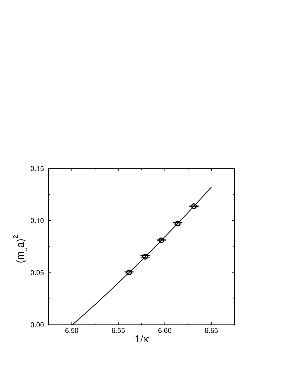
FIG. 19.: Pseudoscalar quarkonium mass squared as a function of $1/\kappa$ for $\beta$ of 6.17 on the lattice $24^{2}\times 20\times 32$.

FIG. 20.: Pseudoscalar quarkonium mass squared as a function of $1/\kappa$ for $\beta$ of 6.4 on the lattice $32^{2}\times 28\times 40$.

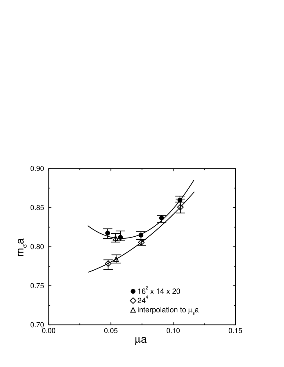
FIG. 21.: Scalar quarkonium mass as a function of quark mass for $\beta$ of 5.93.

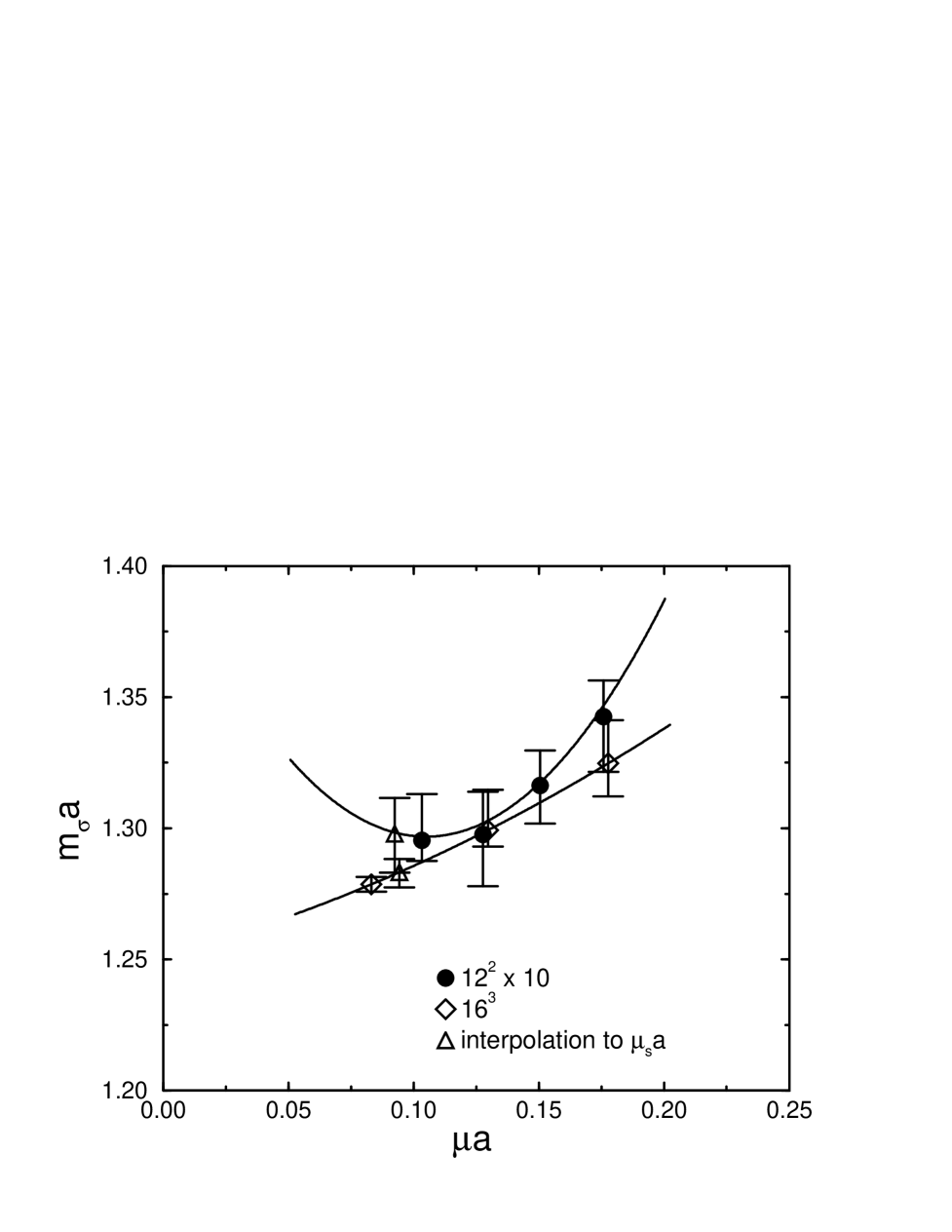
FIG. 22.: Scalar quarkonium mass as a function of quark mass for $\beta$ of 5.7.

FIG. 23.: Scalar quarkonium mass as a function of quark mass for $\beta$ of 6.17.

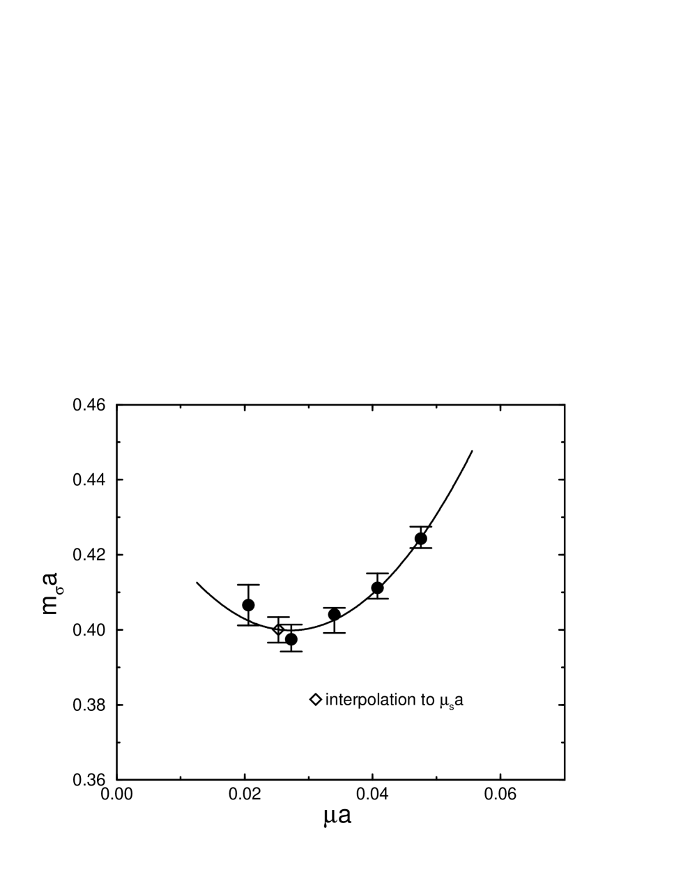
FIG. 24.: Scalar quarkonium mass as a function of quark mass for $\beta$ of 6.4.

FIG. 25.: Lattice spacing dependence and continuum limit of the scalar $s\overline{s}$ mass, continuum limit of the scalar glueball masses, and one sigma upper and lower bounds on observed masses.

FIG. 26.: Scalar glueball effective masses and fitted mass for $\beta$ of 5.70 on a lattice $12^{2}\times 10\times 24$.

FIG. 27.: Scalar glueball effective masses and fitted mass for $\beta$ of 5.93 on a lattice $16^{2}\times 14\times 20$.

FIG. 28.: Scalar glueball effective masses and fitted mass for $\beta$ of 5.93 on a lattice $24^{4}$.

FIG. 29.: Scalar glueball effective masses and fitted mass for $\beta$ of 6.17 on a lattice $24^{2}\times 20\times 32$.

FIG. 30.: Scalar glueball effective masses and fitted mass for $\beta$ of 6.40 on a lattice $32^{2}\times 28\times 40$.

FIG. 31.: Effective mixing energy and fitted mixing energy for $\beta$ of 5.93 and $\kappa$ of 0.1554 on a lattice $16^{2}\times 14\times 20$.

FIG. 32.: Effective mixing energy and fitted mixing energy for $\beta$ of 5.93 and $\kappa$ of 0.1562 on a lattice $16^{2}\times 14\times 20$.

FIG. 33.: Effective mixing energy and fitted mixing energy for $\beta$ of 5.93 and $\kappa$ of 0.1567 on a lattice $16^{2}\times 14\times 20$.

FIG. 34.: Effective mixing energy and fitted mixing energy for $\beta$ of 5.93 and $\kappa$ of 0.1554 on a lattice $24^{4}$.

FIG. 35.: Effective mixing energy and fitted mixing energy for $\beta$ of 5.93 and $\kappa$ of 0.1567 on a lattice $24^{4}$.

FIG. 36.: Effective mixing energy and fitted mixing energy for $\beta$ of 6.40 and $\kappa$ of 0.1491 on a lattice $32^{2}\times 28\times 40$.

FIG. 37.: Effective mixing energy and fitted mixing energy for $\beta$ of 6.40 and $\kappa$ of 0.1494 on a lattice $32^{2}\times 28\times 40$.

FIG. 38.: Effective mixing energy and fitted mixing energy for $\beta$ of 6.40 and $\kappa$ of 0.1497 on a lattice $32^{2}\times 28\times 40$.

FIG. 39.: Glueball-quarkonium mixing energy as a function of quark mass for $\beta$ of 5.93.

FIG. 40.: Glueball-quarkonium mixing energy as a function of quark mass for $\beta$ of 5.70.

FIG. 41.: Glueball-quarkonium mixing energy as a function of quark mass for $\beta$ of 6.17.

FIG. 42.: Glueball-quarkonium mixing energy as a function of quark mass for $\beta$ of 6.40.

FIG. 43.: Lattice spacing dependence and continuum limit of the glueball-quarkonium mixing energy $E(\mu_{s})$ and of the ratio $E(\mu_{n})/E(\mu_{s})$.

REFERENCES

- [1] Present address: T-8, LANL, Los Alamos, NM 87545.
- [2] J. Sexton, A. Vaccarino and D. Weingarten, Phys. Rev. Lett. 75, 4563 (1995).
- [3] A. Vaccarino and D. Weingarten, to appear in Phys. Rev. D.
- [4] H. Chen, J. Sexton, A. Vaccarino and D. Weingarten, Nucl. Phys. B (Proc. Suppl.) 34, 357 (1994).
- [5] G. Bali, K. Schilling, A. Hulsebos, A. Irving, C. Michael and P. Stephenson, Phys. Lett. B 309, 378 (1993).
- [6] D. Weingarten, Nucl. Phys. B (Proc. Suppl.) 34, 29 (1994).
- [7] C. Morningstar and M. Peardon, Phys. Rev. D56, 4043 (1997); hep-lat/9901004, to appear in Phys. Rev. D.
- [8] M. Brisudova, L. Burakovsky and T. Goldman, LANL preprint LA-UR-97-3794, hep-ph/9712514.
- [9] D. Weingarten, Nucl. Phys. B (Proc. Suppl.) 53, 232 (1997).
- [10] C. Amsler et al., Phys. Lett. B355, 425 (1995).
- [11] C. Amsler and F. Close, Phys. Lett. B353 385 (1995); Phys. Rev. D53, 295 (1996).
- [12] W. Lee and D. Weingarten, Nucl. Phys. B (Proc. Suppl.) 63 A-C, 198 (1998).
- [13] W. Lee and D. Weingarten, Nucl. Phys. B (Proc. Suppl.) 53, 236 (1997).
- [14] M. Boglione and M. Pennington, Phys. Rev. Lett. 79, 1998 (1997).
- [15] W. Lee and D. Weingarten, Phys. Rev. D59, 09508 (1999).
- [16] F. Butler, H. Chen, J. Sexton, A. Vaccarino and D. Weingarten, Nucl. Phys. B 430, 179 (1994).
- [17] A. Abele et al., Phys. Lett. B385, 425 (1996).
- [18] SLAC-PUB-5669, 1991; SLAC-PUB-7163; W. Dunwoodie, private communication.