Glueball Mass Predictions of the Valence Approximation to Lattice QCD

Abstract

We evaluate the infinite volume, continuum limit of glueball masses in the valence (quenched) approximation to lattice QCD. For the lightest scalar and tensor states we obtain masses of $1648\pm 58$ MeV and $2267\pm 104$ MeV, respectively.

I Introduction

In recent articles we described calculations of the infinite volume, continuum limit of scalar and tensor glueball masses in the valence (quenched) approximation to lattice QCD [1, 2]. For a single value of lattice spacing and lattice volume, we reported also a calculation of the the decay coupling constants of the lightest scalar glueball to pairs of pseudoscalar mesons. The mass and decay calculations combined support the identification of $f_{0}(1710)$ as primarily composed of the lightest scalar glueball [3, 4]. Evaluation of the mass of the lightest scalar quarkonium states and of quarkonium-glueball mixing amplitudes [5] then yield a glueball component for $f_{0}(1710)$ of $73.8\pm 9.5$ %. In the present article, we describe the glueball mass data of Ref. [1] in greater detail along with an improved evaluation of the mass predictions which follow from these data. For the scalar and tensor glueball masses we obtain $1648\pm 58$ MeV and $2267\pm 104$ MeV, respectively.

The valence approximation, on which our results depend, may be viewed as replacing the momentum dependent color dielectric constant arising from quark-antiquark vacuum polarization with its zero-momentum limit [6] and, for flavor singlet mesons, shutting off transitions between valence quark-antiquark pairs and gluons. The valence approximation is expected to be fairly reliable for low lying flavor nonsinglet hadron masses, which are determined largely by the low momentum behavior of the chromoelectric field. This expectation is supported by recent valence approximation calculations [7, 8] of the masses of the lowest flavor multiplets of spin 1/2 and 3/2 baryons and pseudoscalar and vector mesons. The predicted masses are all within about 10% of experiment. For the lowest valence approximation glueball masses, the error arising from the valence approximation’s omission of the momentum dependence of quark-antiquark vacuum polarization we thus also expect to be 10% or less. Refs. [2, 9] show this error should tend to lower valence approximation masses below those of full QCD. For flavor singlet configurations whose quantum numbers, if realized as quarkonium, require nonzero orbital angular momentum, it is shown in Ref. [2] that the additional error arising from the valence approximation’s suppression of transitions between valence quark-antiquark pairs and gluons is likely to introduce an additional error of the order of 5% or less. For the lowest scalar glueball this error is examined in detail in Ref. [5] and found to shift the valence approximation mass by about 5% below its value in full QCD. It is perhaps useful to mention that, for glueball masses, the valence approximation simply amounts to a reinterpretation of the predictions of pure gauge theory.

In Section II we define a family of operators used to construct glueball propagators. In Section III we describe the set of lattices on which propagators were evaluated and the algorithms we used to generate gauge configurations and estimate error bars. In Sections IV and V we present our results for scalar and tensor glueball propagators, respectively, and masses extracted from these propagators. In Section VI we estimate the difference between the scalar and tensor masses we obtain in finite volumes and the corresponding infinite volume limits. In Section VII we extrapolate scalar and tensor masses to their continuum limits. In Section VIII we compare our calculations with work by other groups [10, 11]. For combined world average valence approximation scalar and tensor glueball masses we obtain $1656\pm 47$ MeV and $2302\pm 62$ MeV, respectively.

II Smeared Operators

We evaluated glueball propagators using operators built out of smeared link variables. Glueball operators built from link variables with an optimal choice of smearing couple more weakly to excited glueball states than do corresponding operators built from unsmeared links. As a consequence, the plateau in effective mass plots for optimally smeared operators begins at a smaller time separation between source and sink operators, extends over a larger number of time units, and yields a fitted mass with smaller statistical noise than would be obtained from operators made from unsmeared link variables. Examples of the improvements which we obtained by a choice of smeared operators with be given in Section IV and V.

Initially, we constructed smeared operators from gauge links fixed to Coulomb gauge. This method gave adequate results for the largest values of lattice spacing we considered. As the lattice spacing was made smaller, however, we found that the computer time required to gauge fix a large enough ensemble of configurations to obtain useful results became unacceptably large. We then switched to a gauge invariant smearing method. For the lattice sizes used in our extrapolation to the continuum limit, the gauge invariant mass results had statistical uncertainties typically a factor of three smaller than our earlier Coulomb gauge results. In the remainder of the present article we discuss only the gauge invariant results. A summary of our Coulomb gauge mass calculations is given in Ref. [1].

A family of gauge invariant smeared operators we construct following the adaptation in Ref. [12] of the smearing method of Ref. [13]. A related method of gauge invariant smearing is proposed in Refs. [14]. For $n>0$, $\epsilon>0$, we define iteratively a sequence of smeared, space-direction link variable $U_{i}^{n\epsilon}(x)$, with $U_{i}^{0\epsilon}(x)$ given by the unsmeared link variable $U_{i}(x)$. Let $u_{i}^{(n+1)\epsilon}(x)$ be

$$u_{i}^{(n+1)\epsilon}(x) = U_{i}^{n\epsilon}(x)+\epsilon\sum_{j}U_{j}^{n\epsilon}(x)U_{i}^{n\epsilon}(x+\hat{j})[U_{i}^{n\epsilon}(x+\hat{i})]^{\dagger}+$$ (2)

$$\epsilon\sum_{j}[U_{j}^{n\epsilon}(x-\hat{j})]^{\dagger}U_{i}^{n\epsilon}(x-\hat{j})U_{i}^{n\epsilon}(x+\hat{i}-\hat{j}),$$

where the sum is over the two space directions $j$ orthogonal to direction $i$. The projection of $u_{i}^{(n+1)\epsilon}(x)$ into SU(3) defines the new smeared link variable $U_{i}^{(n+1)\epsilon}(x)$.

To find $U_{i}^{(n+1)\epsilon}(x)$ we maximize over SU(3) the target function

$$ReTr\{U_{i}^{(n+1)\epsilon}(x)[u_{i}^{(n+1)\epsilon}(x)]^{\dagger}\}.$$ (3)

The required maximum is constructed by repeatedly applying an algorithm related to the Cabbibo-Marinari-Okawa Monte Carlo method. We begin with $U_{i}^{(n+1)\epsilon}(x)$ chosen to be 1. We then multiply $U_{i}^{(n+1)\epsilon}(x)$ by a matrix in the SU(2) subgroup acting only on gauge index values 1 and 2 chosen to maximize the target function over this subgroup. This multiplication and maximization step is repeated for the SU(2) subgroup acting only on index values 2 and 3, then for the subgroup acting only on index values 1 and 3. The entire three step process is then repeated five times. Five repetitions we found sufficient to produce a $U_{i}^{(n+1)\epsilon}(x)$ satisfactorily close to the true maximum of the target function in Eq.  (3). Iteratively maximizing the target function over SU(2) subgroups turns out to be much easier to program than a direct maximization over all of SU(3). The additional computer time required for this iterative maximization, on the other hand, was a negligible fraction of the total time required for our calculation.

From the $U_{i}^{n\epsilon}(x)$ we construct $W_{kl}^{n\epsilon s}(x)$ by taking the trace of the product of $U_{i}^{n\epsilon}(x)$ around the boundary of an $s\times s$ square of links beginning in the $k$ direction. The sum of $W_{kl}^{n\epsilon s}(x)$ over all sites with a fixed time value $t$ gives the zero-momentum loop variable $W_{kl}^{n\epsilon s}(t)$.

For each triple $(n,\epsilon,s)$, a field coupling the vacuum only to zero-momentum scalars states is

$$S^{n\epsilon s}(t) = \sum_{i\neq j}ReW_{ij}^{n\epsilon s}(t),$$ (4)

where the sums are over space directions $i$ and $j$. A possible choice of the two independent operators coupling the vacuum only to zero-momentum tensor states is

$$T_{1}^{n\epsilon s}(t) = 2ReW_{12}^{n\epsilon s}(t)-ReW_{23}^{n\epsilon s}(t)-ReW_{31}^{n\epsilon s}(t)$$ (5)

$$T_{2}^{n\epsilon s}(t) = \sqrt{3}ReW_{23}^{n\epsilon s}(t)-\sqrt{3}ReW_{31}^{n\epsilon s}(t).$$ (6)

The optimal choice of $(n,\epsilon,s)$ for each operator and lattice spacing will be considered in the next section.

III Lattices, Monte Carlo Algorithm and Error Bars

The set of lattices on which we evaluated scalar and tensor glueball propagators is listed in Table I.

On each lattice, an ensembles of gauge configurations was generated by a combination of the Cabbibo-Marinari-Okawa algorithm and the overrelaxed method of Ref. [15]. To update a gauge link we first performed a microcanonical update in the SU(2) subgroup acting on gauge indices 1 and 2. This was then repeated for the SU(2) subgroup acting on indices 2 and 3, and the subgroup acting on indices 1 and 3. These three update steps were then repeated on each link of the lattice. After four lattice sweeps each consisting of the three microcanonical steps on each link, we carried out one Cabibbo-Marinari-Okawa sweep of the full lattice.

At least 10,000 sweeps were used in each case to generate an initial equilibrium configuration. The number of sweeps skipped between each configuration used to calculate propagators and the total number of configurations in each ensemble are listed in the third and fourth columns, respectively, of Table I. Although the number of sweeps skipped in each case was not sufficient to permit successive configurations to be treated as statistically independent, we found successive configurations to be sufficiently independent to justify the cost of evaluating glueball operators.

For the propagators, effective masses and fitted masses to be discussed in Sections IV and V, we determined statistical uncertainties by the bootstrap method [16]. The bootstrap algorithm can be applied directly, however, only to determine the uncertainties in quantities obtained from an ensemble whose individual members are statistically independent. We therefore partitioned each ensemble of correlated gauge configurations into successive disjoint bins with a fixed bin size. Bootstrap ensembles were then formed by randomly choosing a number of entire bins equal to the number of bins in the original partitioned ensemble. For bins sufficiently large, propagator averages found on distinct bins will be nearly independent. It follows that for large enough bins, the binned bootstrap estimate of errors will be reliable. It is not hard to show that once bins are made large enough to produce nearly independent bin averages, further increases in bin size will leave bootstrap error estimates nearly unchanged. The only variation in errors as the bin size is increased further will come from statistical fluctuations in the error estimates themselves. To determine the required bin size for a particular error estimate to be reliable we applied the bootstrap method repeatedly with progressively larger bin sizes until the estimated error became nearly independent of bin size. The final bin size we adopted for each lattice, chosen to be large enough for all of the error estimates done on that lattice, is given in fifth column of Table I.

IV Scalar Propagators and Masses

From the scalar operator of Eq. 4, a propagator for scalars is defined to be

$$P^{n\epsilon s}_{S}(t_{1}-t_{2})=<S^{n\epsilon s}(t_{1})S^{n\epsilon s}(t_{2})>-<S^{n\epsilon s}(t_{1})><S^{n\epsilon s}(t_{2})>.$$ (7)

To reduce statistical noise, $P^{n\epsilon s}_{S}(t_{1}-t_{2})$ is then averaged over reflections and time direction displacements of $t_{1}$ and $t_{2}$.

The collection of values of smearing iterations n, smearing parameter $\epsilon$, and loop size $s$ for which propagators were evaluated for each lattice are given in Table II. At $\beta$ of 5.70, and at $\beta$ of 5.93 on the lattice $16^{3}\times 24$, we ran with relatively larger ranges of parameters to try to find values which coupled efficiently to the lightest scalar glueball. For other lattices, the parameter range was then narrowed to choices which, in physical units, were about the same as the value range which gave best results at $\beta$ of 5.93.

From the existence of a self-adjoint, positive, bounded transfer matrix for lattice QCD, it follows that a spectral resolution can be constructed for $P^{n\epsilon s}_{S}(t)$,

$$P^{n\epsilon s}_{S}(t) = \sum_{i}Z_{i}\{exp(-E_{i}t)+exp[-E_{i}(L-t)]\},$$ (8)

$$Z_{i} = |<i|S^{n\epsilon s}(0)|vacuum>|^{2},$$ (9)

where the sum is over all zero-momentum, scalar states $<i|$, $E_{i}$ is the energy of $<i|$, and $L$ is the lattice period in the time direction. For large values of $t$ and $L$, the sum in Eq. (8) approaches the asymptotic form

$$P^{n\epsilon s}_{S}(t)\rightarrow Z\{exp(-mt)+exp[-m(L-t)]\}$$ (10)

where $m$ is the smallest $E_{i}$ and thus the mass of the lightest scalar glueball and $Z$ is the corresponding $Z_{i}$. Fitting $P^{n\epsilon s}_{S}(t)$ to the asymptotic form in Eq. (10) at $t$ and $t+1$ gives the scalar effective mass $m(t)$, which at large $t$ approaches $m$.

To extract values of $m$ from our data sets, we began by examining effective mass graphs to find combinations of $n$ and $s$ for which $m(t)$ shows a plateau at $t$ values for which we have data, and to determine which of these combination of $n$ and $s$ has the best plateaus.

Among the data sets used in our final extrapolation of the scalar mass to zero lattice spacing, we included the largest range of values of $n$ and $s$ for the lattice $16^{3}\times 24$ with $\beta$ of 5.93. Scalar effective masses obtained for this case with $n$ of $5$ and $s$ of $3-7$ are shown in Figures 1 - 5, respectively. As the loop size $s$ is increased, initially the effective mass graphs become flatter, as shown, for example, by a decrease in the difference between $m(0)$ and $m(2)$. It follows that the relative coupling of the corresponding operators to the lightest scalar glueball increases with $s$. Beyond $s$ of 5, however, this trend reverse. Thus, as might be expected, the relative coupling to the lightest state becomes weaker again when the loop is made too large. For $s$ of 7 the effective mass graph shows no sign of becoming flat even at the largest $t$ for which we have statistically significant data. For $n$ of 5, the best coupling to the lightest state appears to occur with $s$ of 4 or 5. For $s$ fixed at 4, Figure 2 and Figures 6 - 8 show the variation in the effective mass graph as $n$ runs from 5 to 8, respectively. The difference between $m(0)$ and $m(2)$ is least at $n$ of 6 and then grows again as $n$ is raised toward 8.

In Figures 1 - 8 the statistical uncertainty in effective masses grows as $t$ is made larger and tends to grow also if $n$ or $s$ is increased. Both of these phenomena are explained by the discussion in Ref. [17] of the statistical uncertainty in propagators.

Figures 9 - 13 show scalar effective masses for the each of the values of lattice size and $\beta$ listed in Table I. The parameters $n$ and $s$ for the data in Figures 9 - 13 are chosen, for each lattice and $\beta$, from among the set which couple best to the lightest scalar.

For each combination of lattice size and $\beta$, we determined a final value of the scalar mass from the collection of propagators for which the effective mass graph showed at least some evidence of a plateau at large $t$. For several different choices of $t$ interval, each of these propagators was fitted to the asymptotic form in Eq. (10) by minimizing the fit’s correlated $\chi^{2}$. The upper limit of each fitting interval $t_{max}$ we fixed at the largest $t$ for which we had statistically significant propagator data. The lower limit of the fitting interval $t_{min}$ was then progressively increased from 1 to $t_{max}-2$. As $t_{min}$ was increased, the fitted mass and the fit’s $\chi^{2}$ per degree of freedom both generally decreased and the statistical error bar increased. For each $n$ and $s$, the final choice of $t_{min}$ we took to be the smallest value for which the corresponding mass was within the error bars of all the fits with the same $n$ and $s$ and larger $t_{min}$. Our intent in this procedure was to extract a mass from the largest time interval for which the propagator for each combination of $n$ and $s$ was consistent with the asymptotic form of Eq. (10).

The solid horizontal lines in Figures 2 - 5 and Figures 6 - 13 show the best fitted mass in each case and extend over the interval of $t$ on which these fits were made. The dashed lines in these figures extend the solid lines to smaller $t$ to show the approach, with increasing $t$, of effective masses to the final mass values.

For the lattice $16^{3}\times 24$ with $\beta$ of 5.93, Tables III - VI show the results of our fits for all the combination of $n$, $s$, $t_{min}$ and $t_{max}$ which we examined. The best choice of $t_{min}$ and $t_{max}$ turned out to be 2 and 8, respectively, for all $n$ and $s$. Tables VII - XI show the fitted masses found with the best choice of $t_{min}$ and $t_{max}$ for all the lattice sizes, $\beta$, $n$ and $s$ for which our effective mass data showed a plateau at large $t$.

As expected, for each lattice size and $\beta$, the fitted masses in Tables VII - XI vary with $n$ and $s$ by an amount generally less than the statistical uncertainty in each mass. There is also a weak tendency for masses to fall initially with increasing $n$ and $s$, as the corresponding operator’s relative coupling to the lightest glueball increases. Then, in some cases, when $n$ and $s$ become too large the coupling to the lightest state decreases, the fitted masses show some tendency to rise again. To reduce this small remaining statistical uncertainty and systematic bias, our final value of mass for each lattice size and $\beta$ was obtained by an additional fit of a single common mass to a set of masses from a range of several $n$ and $s$. The common mass was chosen to minimize the correlated $\chi^{2}$ of the fit of the common mass to the collection of different best mass values. The correlation matrix among the best mass values was determined by the bootstrap method. The set of $n$ and $s$ used in each final fit was chosen by examining a decreasing sequence of sets, starting with all $n$ and $s$, and progressively eliminating the smallest and largest $n$ and $s$ until a $\chi^{2}$ per degree of freedom below 2.0 was obtained. The final fit was taken from the largest set of channels yielding a $\chi^{2}$ below 2.0. If several sets of equal size gave $\chi^{2}$ per degree of freedom below 2.0, we chose among these the set with smallest $\chi^{2}$ per degree of freedom. Tables XII- XVI show these combined fits and the set of $n$ and $s$ chosen for the final mass value for each lattice and $\beta$. In all of these tables, it is clear that once enough of the largest and smallest $n$ and $s$ are eliminated to give an acceptable $\chi^{2}$ per degree of freedom, the fitted values vary only by small fractions of their statistical uncertainty as additional changes are made in the set of $n$ and $s$. The final mass values are collected in Table XVII.

At several points in Tables XII- XVI, combined fits including several nearby values of $n$ and $s$ yield large $\chi^{2}$ while separate fits to smaller subsets of $n$ and $s$ give nearly equal masses and acceptable $\chi^{2}$. This phenomenon, we have found, does not indicate a problem with our data or our fits and arises instead because propagators with nearby values of $n$ and $s$ in some cases are very highly correlated and yield slightly different masses. A similar problem would arise in trying to fit a single value $x$ to, say, a gaussian random variable $X$ with dispersion 1, and a shifted copy $X+0.0001$. For any choice of $x$ the fit’s $\chi^{2}$ is infinite. Nonetheless, for a Monte Carlo ensemble of 1000 $X$ values, taking $x$ as either $<X>\pm 1/\sqrt{1000}$ or $<X>+0.0001\pm 1/\sqrt{1000}$ is a reliable estimate of the mean of $X$ with systematic error much smaller than the statistical error.

An alternative way to extract a single mass from glueball propagators for a range of $n$, $\epsilon$ and $s$ uses the matrix of propagators

$$M^{k\delta rn\epsilon s}_{S}(t_{1}-t_{2})=<S^{k\delta r}(t_{1})S^{n\epsilon s}(t_{2})>-<S^{k\delta r}(t_{1})><S^{n\epsilon s}(t_{2})>.$$ (11)

For large $t$ and lattice time direction period $L$, $M^{k\delta rn\epsilon s}_{S}(t)$ has the asymptotic form

$$M^{k\delta rn\epsilon s}_{S}(t)\rightarrow Z^{k\delta rn\epsilon s}\{exp(-mt)+exp[-m(L-t)]\}$$ (12)

where $m$ is the mass of the lightest scalar glueball and $Z^{k\delta rn\epsilon s}$ is a matrix independent of $t$. In principle, $M^{k\delta rn\epsilon s}_{S}(t)$ can be extracted from our data and fitted to Eq. (12) to produce a value for $m$. To find the best $m$ and $Z^{k\delta rn\epsilon s}$ by minimizing the fit’s $\chi^{2}$, however, requires the statistical correlation matrix among the fitted $M^{k\delta rn\epsilon s}_{S}(t)$. If we fit, for example, to three choices of $(k,\delta,r)$, three choices of $(n,\epsilon,s)$ and four values of $t$, the correlation matrix has 1296 entries. Our underlying data set is too small to provide reliable entries for such a large correlation matrix. As a consequence the value of $m$ determined this way will have a statistical error which can not be estimated reliably. In practice, we found that the value of $m$ produced by this method was not stabile as we varied the sets of $(m,\delta,r)$ and $(n,\epsilon,s)$ and the range of $t$ used in the fit.

V Tensor Propagators and Masses

A propagator for tensors is defined to be

$$P^{n\epsilon s}_{T}(t_{1}-t_{2})=\sum_{i}[<T_{i}^{n\epsilon s}(t_{1})T_{i}^{n\epsilon s}(t_{2})>-<T_{i}^{n\epsilon s}(t_{1})><T_{i}^{n\epsilon s}(t_{2})>].$$ (13)

where $T_{1}$ and $T_{2}$ are the tensor glueball operators of Eq. (5), and $P^{n\epsilon s}_{T}(t_{1}-t_{2})$ is then averaged over reflections and time direction displacements of $t_{1}$ and $t_{2}$ to reduce statistical noise.

Tensor propagators were found for gauge configuration ensembles and operator parameters listed in Tables I and II. A tensor glueball mass was extracted from propagators by fitting the data to the tensor version of Eq. (10). We obtained a satisfactory tensor glueball mass signal only for the lattices with $\beta$ of 5.93, 6.17 and 6.40. We did not find an acceptable tensor signal at $\beta$ of 5.70. Overall, the statistical errors in the tensor data are larger than those in the scalar data of Section IV and, as a result, the fitting process encounters complications not present in the scalar fits.

Tables XVIII - XXI list tensor masses for each gauge ensemble with $\beta$ of 5.93 and above, for each set of operator parameters in Table II, fitted on one or, in some cases, two choices of time interval. For all fits the high end of the fitting range $t_{max}$ is chosen to be the largest value at which a statistically significant effective mass is found. The low end of the fitting range $t_{min}$ is then progressively increased. The smallest $t_{min}$ yielding a mass within one standard deviation of the masses for all larger $t_{min}$ is selected as the lower bound for an initial choice of the fitting range. For the lattice $16^{3}\times 24$ at $\beta$ of 5.93 and for the lattice $32^{2}\times 30\times 40$ and $\beta$ of 6.40, however, we found that for almost all choices of operator parameters a $t_{min}$ one unit larger than the initial choice yielded a noticeably lower mass. These second values of $t_{min}$ and the corresponding masses are also listed in Tables XIX, and XXI.

Effective mass plots for tensors are shown in Figures 14 - 17, for the four lattices with $\beta$ of 5.93 and larger, for typical choices of operator parameters. The solid line in each figure indicates the mass obtained from a fit over the time interval which the line spans. The dashed line in each figures extend the solid line to smaller $t$ to show the approach of effective masses to the fitted value.

Tables XXII - XXV list tensor masses found by combining, as discussed in Section IV, the masses fitted to various sets of operators and choices of time interval. Table XXII corresponds to the lattices $12^{3}\times 24$ at $\beta$ of 5.93 with fits using the single time interval given in Table XXII. Table XXIV corresponds to the lattice $24^{3}\times 36$ at $\beta$ of 6.17 with fits using the single time interval in Table XX. In Tables XXII and XXIV, all combined fits with acceptable $\chi^{2}$ per degree of freedom give masses consistent with each other to within statistical uncertainties. In each case, the mass corresponding to the largest set with acceptable $\chi^{2}$, marked with an arrow, is chosen as the final value.

Table XXIII for the lattice $16^{3}\times 24$ at $\beta$ of 5.93 shows combined fits using both choices of $t_{min}$ of Table XIX. The combined fits using the smaller $t_{min}$ have unacceptably high $\chi^{2}$ per degree of freedom. For the fits using the larger $t_{min}$ the $\chi^{2}$ is acceptable, and the fitted masses are all consistent with each other within statistical uncertainties. The mass for the largest set of operators with the larger $t_{min}$ is chosen as the final number. Table XXV for the lattice $32^{2}\times 30\times 40$ at $\beta$ of 6.40 also gives combined fits for both $t_{min}$ in Table XXI. Most fits for both $t_{min}$ have acceptable $\chi^{2}$ per degree of freedom. The masses obtained from the larger $t_{min}$ all lie one standard deviation or a bit more below the masses found with the smaller $t_{min}$, however, and all have significantly better $\chi^{2}$ than the fits with the smaller $t_{min}$. The mass found from the largest set of operators for the larger $t_{min}$ is therefore chosen as the final result.

The collection of final tensor masses is listed in Table XXVI.

VI Volume Dependence

We now consider an estimate of the difference between the scalar and tensor glueball masses in Table XVII and XXVI for finite lattice period $L$ and the infinite volume limits of these quantities.

For large values of $L$, scalar $m_{0}(L)$ and tensor $m_{2}(L)$ glueball masses deviate from their infinite volume limits, $m_{0}$ and $m_{2}$, respectively, by [18]

$$m_{s}(L)=m_{s}\{1-g_{s}\frac{exp(\frac{-\sqrt{3}m_{0}L}{2})}{m_{0}L}-O[\frac{exp(-m_{0}L)}{m_{0}L}]\}$$ (14)

where $s$ is 0 or 2. In Ref. [19] for $\beta$ near 6.0, data for $m_{0}(L)$ is shown to fit the two leading terms in Eq. (14) reasonably well at 4 values of $L$ ranging from $6/m_{0}$ to $12/m_{0}$. This result is plausible since for $L$ ranging from $6/m_{0}$ to $12/m_{0}$, the third term in Eq. (14) is smaller than the second by a factor ranging from $O(0.4)$ to $O(0.2)$. For our data at $\beta$ of 5.93, Table XVII shows that $m_{0}$ is above 0.75 so that $L$ of 12 and 16 are larger than $8/m_{0}$ and $12/m_{0}$, respectively. Thus we believe that for the data at $\beta$ of 5.93, the leading two terms of Eq. (14) likely provide a fairly reliable estimate of the $L$ dependence of $m_{0}(L)$ and $m_{2}(L)$.

Fitting the $\beta=5.93$ data in Table XVII to the two leading terms of Eq. (14) yields $m_{0}$ of $0.783\pm 0.012$ and $g_{0}$ of $1500\pm 1100$. In addition a bootstrap calculation yields with 95% probability

$$\frac{m_{0}-m_{0}(16)}{m_{0}}\leq 0.0037.$$ (15)

. At $\beta=5.93$, Table XXVI combined with the leading two terms of Eq. (14) gives $m_{2}$ of $1.236\pm 0.037$ and $g_{2}$ is $1300\pm 1200$. A bootstrap calculation yields with 95% probability

$$\frac{m_{2}-m_{2}(16)}{m_{2}}\leq 0.0048$$ (16)

.

Overall, it appears to us safe to conclude that at $\beta$ of 5.93 the difference between scalar and tensor masses for $L$ of 16 and their infinite volume limits are of the order of 0.5% or less. In Section VII we show that the scalar and tensor glueball masses in Tables XVII and XXVI with $\beta$ of 5.93 and greater and $m_{0}L$ fixed at about 13 are not far from asymptotic scaling. We therefore expect the fractional volume dependent errors found in these masses to be about the same as the errors at $\beta$ of 5.93. Thus the finite volume errors in all masses in Tables XVII and XXVI with $\beta$ of 5.93 and greater and $m_{0}L$ of about 13 should be 0.5% or less.

VII Continuum Limit

The nonzero lattice spacing scalar and tensor glueball masses in lattice units given in Tables XVII and XXVI, respectively, we now convert to physical units and extrapolate to zero lattice spacing.

To convert masses in lattice units to physical units, we divide by a known mass measured in lattice units. One natural choice for this conversion factor is the rho mass $m_{\rho}(a)a$. Values of $m_{\rho}(a)a$ for three of the four $\beta$ in Tables XVII and XXVI are given in Ref. [7]. For the largest $\beta$ in Tables XVII and XXVI, Ref. [7] does not report $m_{\rho}(a)a$. For the three $\beta$ considered in Ref. [7], however, the ratio $[\Lambda^{(0)}_{\overline{MS}}a]/[m_{\rho}(a)a]$ is found to be independent of $\beta$ to within statistical errors. Here $\Lambda^{(0)}_{\overline{MS}}a$ is obtained by the 2-loop Callan-Symanzik equation from $\alpha_{\overline{MS}}$ found from its mean-field improved [20] relation to $\beta$. Since $[\Lambda^{(0)}_{\overline{MS}}a]/[m_{\rho}(a)a]$ is constant within errors, converting to physical units using $\Lambda^{(0)}_{\overline{MS}}a$ then extrapolating to zero lattice spacing should give results nearly equivalent to those found using $m_{\rho}(a)a$. Table XXVII lists, for each $\beta$, the corresponding mean-field improved $\alpha_{\overline{MS}}$ and $\Lambda^{(0)}_{\overline{MS}}a$.

The $\beta$ dependence of valence approximation glueball masses is determined entirely by the pure gauge part of the QCD action. The leading irrelevant operator in the pure gauge plaquette action has lattice spacing dependence of $O(a^{2})$. Thus for scalar and tensor glueball masses $m_{0}$ and $m_{2}$, respectively, we extrapolate to the continuum limit by

$$\frac{m_{s}(a)a}{\Lambda^{(0)}_{\overline{MS}}a} = \frac{m_{s}}{\Lambda^{(0)}_{\overline{MS}}}+C[\Lambda^{(0)}_{\overline{MS}}a]^{2},$$ (17)

where $s$ is 0 or 2.

If $\Lambda^{(0)}_{\overline{MS}}a$ in Eq. (17) were replaced by $m_{\rho}(a)a$, then since the leading irrelevant operator in the quark action has lattice spacing dependence of $O(a)$ it might be argued that the quadratic $O(a^{2})$ term in the equation’s right hand side should be a linear $O(a)$. This in turn would contradict our claim that extrapolation using either $m_{\rho}(a)a$ or $\Lambda^{(0)}_{\overline{MS}}a$ will give nearly equal results. An answer to this objection is that the approximate constancy of $[\Lambda^{(0)}_{\overline{MS}}a]/[m_{\rho}(a)a]$ implies that the $O(a)$ irrelevant contribution to $m_{\rho}(a)a$ is quite small. The constancy of $[\Lambda^{(0)}_{\overline{MS}}a]/[m_{\rho}(a)a]$ as a function of $a$ or equivalently as a function of $\beta$ can not be explained by a cancellation of an $O(a)$ term in $\Lambda^{(0)}_{\overline{MS}}a$ with an $O(a)$ term in $m_{\rho}(a)a$ since $\Lambda^{(0)}_{\overline{MS}}a$ is defined to fulfill the true continuum two-loop Callan-Synamzik equation and itself has no $O(a)$ corrections. The leading correction to the $\beta$ dependence of $\Lambda^{(0)}_{\overline{MS}}a$ is by a multiplicative factor of $[1+O(\beta^{2})]$. If $\Lambda^{(0)}_{\overline{MS}}a$ is replaced by $m_{\rho}(a)a$, any significant $a$ dependence which appears will come from the $O(a^{2})$ term in $m_{s}(a)a$. Thus Eq. (17) even with $m_{\rho}(a)a$ substituted for $\Lambda^{(0)}_{\overline{MS}}a$ will remain correct.

The scalar data of Tables XVII combined with $\Lambda^{(0)}_{\overline{MS}}a$ of Table XXVII fitted to Eq. (17) at the three largest $\beta$ is shown in Figure 18. The predicted continuum limit $m_{0}/\Lambda^{(0)}_{\overline{MS}}$ is $7.016\pm 0.167$. The fit in Figure 18 has a $\chi^{2}$ of 0.6 over a range in which the term $[\Lambda^{(0)}_{\overline{MS}}a]^{2}$ varies by more than a factor of 3.4. The variation of $[m_{s}(a)a]/[\Lambda^{(0)}_{\overline{MS}}a]$ over the fitting range, however, is only slight. Each of the three nonzero lattice spacing values of $[m_{s}(a)a]/[\Lambda^{(0)}_{\overline{MS}}a]$ is within 1.6 standard deviations of the extrapolated zero lattice spacing result. Thus we believe the extrapolation to zero lattice spacing is quite reliable and would expect the predicted continuum mass to be not very different from what would be obtained by any other reasonable, smooth extrapolation of the data.

The tensor data of Tables XXVI combined with $\Lambda^{(0)}_{\overline{MS}}a$ of Table XXVII fitted to Eq. (17) at the three largest $\beta$, the only $\beta$ for which tensor masses were found, is shown in Figure 19. The predicted continuum limit $m_{2}/\Lambda^{(0)}_{\overline{MS}}$ is $9.65\pm 0.36$. The fit in Figure 19 has a $\chi^{2}$ of 0.8, while, as before, the term $[\Lambda^{(0)}_{\overline{MS}}a]^{2}$ in Eq. (17) varies by more than a factor of 3.4 over the fitting range.

To obtain scalar and tensor glueball masses in units of MeV, we combine the continuum limit $\Lambda^{(0)}_{\overline{MS}}/m_{\rho}$ of $0.305\pm 0.008$ [7] with $m_{\rho}$ of 770 MeV to give $\Lambda^{(0)}_{\overline{MS}}$ of $234.9\pm 6.2$ MeV. The scalar glueball mass becomes $1648\pm 58$ MeV and the tensor mass becomes $2267\pm 104$ MeV. The continuum limit results are summarized in Table XXVIII.

For $\Lambda^{(0)}_{\overline{MS}}/m_{\rho}$ we take the value given in Ref. [7] for a lattice with period of about 2.4 fermi. For the rho mass obtained at $\beta$ of 5.7 from a combination of propagators for rho operators with smearing parameters 0, 1 and 2, the 2.4 fermi result differs from the result for period 3.6 fermi by a bit over one standard deviation. This difference appears to be largely a consequence of a slightly poorer separtion of the rho component of the propagator from excited state components in the 2.4 fermi rho mass calculation than in the 3.6 fermi calculation [21]. For the rho operator with smearing parameter 4, which couples more weakly to excited states, the difference at $\beta$ of 5.7 between 2.4 fermi and 3.6 fermi predictions is much less than one standard deviation. Thus overall it appears to us reasonable to take the 2.4 fermi calculations as the infinite volume limit, within statistical errors. The continuum limit values of $\Lambda^{(0)}_{\overline{MS}}/m_{\rho}$ for the the data combining smearings 0, 1 and 2 and for the data from smearing 4 are nearly identical.

VIII Comparison with Other Results

An independent calculation of the infinite volume, continuum limit of the valence approximation to several glueball masses is reported in Ref. [10]. A second, more recent, calculation appears in Ref. [11]. A comparison of Ref. [10] with the original analysis [1] of our results appears in Ref. [2].

The calculation of Ref. [10] uses the same plaquette action we use but takes a different set of glueball operators. The gauge field ensembles of Ref. [10] range from 1000 to 3000 configurations. For the scalar and tensor masses Ref. [10] reports $1550\pm 50$ MeV and $2270\pm 100$ MeV, respectively. The predicted zero lattice spacing masses are not actually found by extrapolation to zero lattice spacing, but are obtained instead from calculations at $\beta$ of 6.40 of glueball masses in units of the square root of string tension, $\sqrt{\sigma}$, then converted to MeV using an assumed $\sqrt{\sigma}$ of 440 MeV with zero uncertainty. The uncertainties given in the masses are entirely the uncertainties in the $\beta$ of 6.40 calculations of masses in units of $\sqrt{\sigma}$ and are thus missing at least a contribution from the uncertainty in $\sqrt{\sigma}$. A graph shown in Ref. [10] suggests that the $\beta$ of 6.40 value of $[m_{0}(a)a]/[\sqrt{\sigma(a)}a]$ is about 50 MeV below the data’s zero lattice spacing limit. An additional error of $\pm 50$ MeV in the scalar mass is therefore proposed in Ref. [10] as a consequence of the absence of extrapolation to zero lattice spacing. Since $[m_{0}(a)a]/[\sqrt{\sigma(a)}a]$ of Ref. [10] is clearly rising as lattice spacing falls, it does not appear to us that a symmetric error of $\pm 50$ MeV an accurate representation of the effect of the absence of extrapolation. If the statistical error and extrapolation error in the scalar mass are, nonetheless, taken at face value and combined the result is a prediction of $1550\pm 71$ MeV. No estimate is given for the extrapolation error in the tensor mass, which is found to be only weakly dependent on lattice spacing if measured in units of $\sqrt{\sigma}$. A scalar mass of $1550\pm 71$ MeV is a bit over one standard deviations below the result $1648\pm 58$ MeV in Table XXVIII, while the tensor mass of $2270\pm 100$ MeV is in close agreement with our value of $2267\pm 104$ MeV.

If the continuum limit of the Ref. [10] data is found by extrapolation to zero lattice spacing of $[m_{0}(a)a]/[\Lambda^{(0)}_{\overline{MS}}a]$, following Section VII, the result for $m_{0}/\Lambda^{(0)}_{\overline{MS}}$ is $6.67\pm 0.33$. Converted to MeV using $\Lambda^{(0)}_{\overline{MS}}$ of $234.9\pm 6.2$ MeV, $m_{0}$ becomes $1567\pm 88$ MeV. This value is less than a standard deviation below the prediction $1648\pm 58$ MeV in Table XXVIII.

The calculation of Ref. [11] uses an improved action with time direction lattice spacing chosen smaller than the space direction. The gauge field ensembles range in size from 4000 to 10000 configurations. Masses measured in units of the parameter $r_{0}^{-1}$ [22] are extrapolated to zero lattice spacing, then converted to MeV using a value of $r_{0}^{-1}$ found by extrapolation of $r_{0}^{-1}/m_{\rho}$ to zero lattice spacing. As a result of working at relatively large values of lattice spacing, some ambiguity is encountered in matching the scalar mass’s lattice spacing dependence to the small lattice spacing asymptotic behavior expected for the improved action. Taking this uncertainty into account, the scalar mass is predicted to be $1730\pm 94$ MeV. The tensor mass, for which the extrapolation to zero lattice spacing encounters no problem, is predicted to be $2400\pm 122$ MeV. Both numbers are a bit under one standard deviation above the predictions in Table XXVIII. For the ratio $m_{2}/m_{0}$ Ref. [11] predicts $1.39\pm 0.04$, in good agreement with the value $1.375\pm 0.066$ in Table XXVIII. Thus the difference between Table XXVIII and Ref. [11] is almost entirely a discrepancy in overall mass scale.

Combining our extrapolation of $6.67\pm 0.33$ for the data in Ref. [10] with $7.016\pm 0.167$ in Table XXVIII gives $6.95\pm 0.15$ for $m_{0}/\Lambda^{(0)}_{\overline{MS}}$, thus $1631\pm 55$ MeV. Combining $1631\pm 55$ MeV with $1730\pm 94$ MeV of Ref. [11] gives a world average valence approximation scalar mass of $1656\pm 47$ MeV. This number is consistent with the unmixed scalar mass of $1622\pm 29$ MeV found in Ref. [5] taking the observed states $f_{0}(1710)$, $f_{0}(1500)$ and $f_{0}(1400)$ as the mixed versions of the scalar glueball and the two isoscalar spin zero quarkonium states, respectively. The state $f_{0}(1710)$ in this calculation is assigned a glueball component of $73.8\pm 9.5$ %. Combining $2270\pm 100$ MeV, $2267\pm 104$ MeV and $2400\pm 122$ MeV gives a world average valence approximation tensor mass of $2302\pm 62$ MeV.

$\beta$	lattice	skip	count	bin
5.70	$16^{3}\times 24$	50	8,094	8
5.93	$12^{3}\times 24$	25	48,278	16
	$16^{3}\times 24$	25	30,640	16
6.17	$24^{3}\times 36$	25	31,150	16
6.40	$30\times 32^{2}\times 40$	25	25,440	16

TABLE I.: Configurations analyzed.

$\beta$	lattice	n	$\epsilon$	s
5.70	$16^{3}\times 24$	$3-10$	0.25	$1-4$
5.93	$12^{3}\times 24$	$5-7$	1.00	$4-6$
	$16^{3}\times 24$	$5-8$	1.00	$3-7$
6.17	$24^{3}\times 36$	7,8	1.00	$7-10$
6.40	$30\times 32^{2}\times 40$	6,8	1.00	$7-11$

TABLE II.: Glueball operator parameters.

$n$	$s$	$t_{min}$	$t_{max}$	mass	$\chi^{2}/d.o.f.$
5	4	1	8	$0.827\pm 0.006$	2.26
5	4	2	8	$0.792\pm 0.013$	1.14
5	4	3	8	$0.817\pm 0.029$	1.22
5	4	4	8	$0.831\pm 0.068$	1.61
5	5	1	8	$0.810\pm 0.006$	0.85
5	5	2	8	$0.791\pm 0.013$	0.55
5	5	3	8	$0.798\pm 0.028$	0.67
5	5	4	8	$0.767\pm 0.059$	0.80
5	6	1	8	$0.824\pm 0.007$	1.32
5	6	2	8	$0.793\pm 0.014$	0.58
5	6	3	8	$0.785\pm 0.031$	0.71
5	6	4	8	$0.721\pm 0.066$	0.57

TABLE III.: Fitted scalar glueball mass in lattice units for various choices of $n$, $s$ and fitting range for the lattice $16^{3}\times 24$ at $\beta=5.93$.

$n$	$s$	$t_{min}$	$t_{max}$	mass	$\chi^{2}/d.o.f.$
6	4	1	8	$0.815\pm 0.006$	1.82
6	4	2	8	$0.785\pm 0.012$	0.96
6	4	3	8	$0.813\pm 0.027$	0.90
6	4	4	8	$0.806\pm 0.064$	1.20
6	5	1	8	$0.800\pm 0.006$	0.70
6	5	2	8	$0.785\pm 0.012$	0.50
6	5	3	8	$0.799\pm 0.027$	0.55
6	5	4	8	$0.755\pm 0.054$	0.53
6	6	1	8	$0.811\pm 0.006$	0.96
6	6	2	8	$0.788\pm 0.013$	0.51
6	6	3	8	$0.789\pm 0.028$	0.64
6	6	4	8	$0.722\pm 0.060$	0.39

TABLE IV.: Fitted scalar glueball mass in lattice units for various choices of $n$, $s$ and fitting range for the lattice $16^{3}\times 24$ at $\beta=5.93$.

$n$	$s$	$t_{min}$	$t_{max}$	mass	$\chi^{2}/d.o.f.$
7	4	1	8	$0.803\pm 0.006$	1.41
7	4	2	8	$0.777\pm 0.012$	0.70
7	4	3	8	$0.809\pm 0.026$	0.48
7	4	4	8	$0.782\pm 0.059$	0.58
7	5	1	8	$0.792\pm 0.006$	0.61
7	5	2	8	$0.779\pm 0.012$	0.45
7	5	3	8	$0.798\pm 0.027$	0.42
7	5	4	8	$0.746\pm 0.052$	0.25
7	6	1	8	$0.800\pm 0.006$	0.75
7	6	2	8	$0.783\pm 0.013$	0.47
7	6	3	8	$0.793\pm 0.027$	0.55
7	6	4	8	$0.723\pm 0.056$	0.20

TABLE V.: Fitted scalar glueball mass in lattice units for various choices of $n$, $s$ and fitting range for the lattice $16^{3}\times 24$ at $\beta=5.93$.

$n$	$s$	$t_{min}$	$t_{max}$	mass	$\chi^{2}/d.o.f.$
8	4	1	8	$0.789\pm 0.007$	0.97
8	4	2	8	$0.765\pm 0.013$	0.49
8	4	3	8	$0.803\pm 0.031$	0.18
8	4	4	8	$0.754\pm 0.063$	0.04
8	5	1	8	$0.784\pm 0.006$	0.63
8	5	2	8	$0.768\pm 0.012$	0.40
8	5	3	8	$0.791\pm 0.029$	0.31
8	5	4	8	$0.748\pm 0.055$	0.23
8	6	1	8	$0.791\pm 0.006$	0.77
8	6	2	8	$0.775\pm 0.013$	0.57
8	6	3	8	$0.797\pm 0.028$	0.54
8	6	4	8	$0.716\pm 0.057$	0.04

TABLE VI.: Fitted scalar glueball mass in lattice units for various choices of $n$, $s$ and fitting range for the lattice $16^{3}\times 24$ at $\beta=5.93$.

$n$	$s$	$t_{min}$	$t_{max}$	mass	$\chi^{2}/d.o.f.$
4	1	1	5	$0.971\pm 0.019$	0.23
4	2	1	5	$0.959\pm 0.017$	0.35
4	3	1	5	$0.952\pm 0.016$	0.39
4	4	1	5	$0.984\pm 0.023$	0.26
5	1	1	5	$0.964\pm 0.018$	0.26
5	2	1	5	$0.956\pm 0.017$	0.29
5	3	1	5	$0.953\pm 0.017$	0.23
5	4	1	5	$0.983\pm 0.020$	0.15
6	1	1	5	$0.958\pm 0.017$	0.27
6	2	1	5	$0.954\pm 0.017$	0.23
6	3	1	5	$0.956\pm 0.017$	0.13
6	4	1	5	$0.985\pm 0.020$	0.09

TABLE VII.: Fitted scalar glueball mass in lattice units using the best $t_{min}$ and $t_{max}$ for various choices of $n$ and $s$ for the lattice $16^{3}\times 24$ at $\beta$ of $5.70$

$n$	$s$	$t_{min}$	$t_{max}$	mass	$\chi^{2}/d.o.f.$
5	4	3	7	$0.752\pm 0.021$	1.30
5	5	3	7	$0.737\pm 0.020$	1.01
5	6	3	7	$0.747\pm 0.022$	0.46
6	4	3	7	$0.754\pm 0.020$	0.97
6	5	3	7	$0.742\pm 0.020$	0.68
6	6	2	7	$0.772\pm 0.010$	0.51
6	6	3	7	$0.751\pm 0.022$	0.29
7	4	3	7	$0.757\pm 0.020$	0.72
7	5	3	7	$0.747\pm 0.020$	0.42
7	6	2	7	$0.772\pm 0.010$	0.28
7	6	3	7	$0.756\pm 0.021$	0.16

TABLE VIII.: Fitted scalar glueball mass in lattice units using the best $t_{min}$ and $t_{max}$ for various choices of $n$ and $s$ for the lattice $12^{3}\times 24$ at $\beta$ of $5.93$

$n$	$s$	$t_{min}$	$t_{max}$	mass	$\chi^{2}/d.o.f.$
5	4	2	8	$0.792\pm 0.013$	1.14
5	5	2	8	$0.791\pm 0.013$	0.55
5	6	2	8	$0.793\pm 0.014$	0.58
6	4	2	8	$0.785\pm 0.012$	0.96
6	5	2	8	$0.785\pm 0.012$	0.50
6	6	2	8	$0.788\pm 0.013$	0.51
7	4	2	8	$0.777\pm 0.012$	0.70
7	5	2	8	$0.779\pm 0.012$	0.45
7	6	2	8	$0.783\pm 0.013$	0.47
8	4	2	8	$0.765\pm 0.013$	0.49
8	5	2	8	$0.768\pm 0.012$	0.40
8	6	2	8	$0.775\pm 0.013$	0.57

TABLE IX.: Fitted scalar glueball mass in lattice units using the best $t_{min}$ and $t_{max}$ for various choices of $n$ and $s$ for the lattice $16^{3}\times 24$ at $\beta$ of $5.93$

$n$	$s$	$t_{min}$	$t_{max}$	mass	$\chi^{2}/d.o.f.$
7	7	4	9	$0.570\pm 0.018$	0.22
7	8	4	9	$0.561\pm 0.020$	0.14
7	9	4	9	$0.554\pm 0.024$	0.30
7	10	4	9	$0.540\pm 0.030$	0.38
8	7	4	9	$0.562\pm 0.019$	0.18
8	8	4	9	$0.551\pm 0.018$	0.17
8	9	4	9	$0.545\pm 0.021$	0.10
8	10	4	9	$0.534\pm 0.027$	0.17

TABLE X.: Fitted scalar glueball mass in lattice units using the best $t_{min}$ and $t_{max}$ for various choices of $n$ and $s$ for the lattice $24^{3}\times 36$ at $\beta$ of $6.17$

$n$	$s$	$t_{min}$	$t_{max}$	mass	$\chi^{2}/d.o.f.$
6	7	4	12	$0.461\pm 0.013$	0.50
6	8	4	12	$0.446\pm 0.012$	0.57
6	9	3	12	$0.448\pm 0.008$	0.85
6	10	3	12	$0.435\pm 0.009$	0.57
6	11	3	12	$0.431\pm 0.010$	0.29
8	7	4	12	$0.456\pm 0.013$	0.37
8	8	4	12	$0.447\pm 0.012$	0.54
8	9	4	12	$0.434\pm 0.011$	0.53
8	10	3	12	$0.433\pm 0.008$	0.61
8	11	4	12	$0.417\pm 0.013$	0.63

TABLE XI.: Fitted scalar glueball mass in lattice units using the best $t_{min}$ and $t_{max}$ for various choices of $n$ and $s$ for the lattice $30\times 32^{2}\times 40$ at $\beta$ of $6.40$

$n$	$s$	mass	$\chi^{2}/d.o.f.$
4,5,6	1,2,3,4	$0.978\pm 0.013$	4.85
4,5,6	1,2,3	$0.973\pm 0.014$	3.70
4,5	1,2,3,4	$0.975\pm 0.014$	5.39
5,6	1,2,3,4	$0.974\pm 0.014$	6.46
4	1,2,3,4	$0.965\pm 0.014$	8.95
5	1,2,3,4	$0.964\pm 0.015$	9.90
6	1,2,3,4	$0.966\pm 0.015$	10.20
4,5,6	2,3	$0.973\pm 0.014$	5.07
5,6	2,3,4	$0.973\pm 0.014$	7.25
5	2,3,4	$0.964\pm 0.015$	14.80
4,5	2,3	$0.966\pm 0.014$	3.46
5,6	2,3	$0.969\pm 0.014$	6.04
4,5	2	$0.957\pm 0.015$	1.70
4,5	3	$0.953\pm 0.015$	0.20
5,6	3	$0.953\pm 0.015$	1.67
5,6	2	$0.955\pm 0.015$	0.35
4	2,3	$0.955\pm 0.014$	1.36
5	2,3	$0.954\pm 0.015$	0.22
6	2,3	$0.955\pm 0.015$	0.11	$\leftarrow$

TABLE XII.: Scalar glueball mass in lattice units found by combined fits to sets of $n$ and $s$ for the lattice $16^{3}\times 24$ at $\beta$ of $5.70$. The final set chosen is indicated by an arrow.

$n$	$s$	mass	$\chi^{2}/d.o.f.$
5,6,7	4,5,6	$0.752\pm 0.020$	2.35
5,6,7	4,5	$0.750\pm 0.019$	1.75
5,6,7	5,6	$0.747\pm 0.020$	0.98	$\leftarrow$
5,6	4,5,6	$0.752\pm 0.019$	3.72
6,7	4,5,6	$0.751\pm 0.020$	3.67
5,6	4,5	$0.749\pm 0.019$	2.88
5,6	5,6	$0.745\pm 0.020$	1.41
6,7	4,5	$0.747\pm 0.020$	2.52
6,7	5,6	$0.746\pm 0.020$	1.48
6	5,6	$0.742\pm 0.020$	1.19
7	5,6	$0.748\pm 0.020$	1.24

TABLE XIII.: Scalar glueball mass in lattice units found by combined fits to sets of $n$ and $s$ for the lattice $12^{3}\times 24$ at $\beta$ of $5.93$. The final set chosen is indicated by an arrow.

$n$	$s$	mass	$\chi^{2}/d.o.f.$
5,6,7,8	4,5,6	$0.781\pm 0.011$	1.90	$\leftarrow$
5,6,7,8	4,5	$0.779\pm 0.011$	2.77
5,6,7,8	5,6	$0.776\pm 0.012$	1.99
5,6,7	4,5,6	$0.779\pm 0.011$	2.14
5,6,7	4,5	$0.778\pm 0.012$	3.24
5,6,7	5,6	$0.776\pm 0.012$	2.29
6,7,8	4,5,6	$0.782\pm 0.011$	2.32
6,7,8	4,5	$0.780\pm 0.011$	3.50
6,7,8	5,6	$0.777\pm 0.012$	2.00
6,7	4,5,6	$0.778\pm 0.011$	3.01
7,8	4,5,6	$0.778\pm 0.012$	1.68
6	4,5,6	$0.786\pm 0.012$	0.21
7	4,5,6	$0.779\pm 0.012$	0.32
8	4,5,6	$0.771\pm 0.012$	0.86

TABLE XIV.: Scalar glueball mass in lattice units found by combined fits to sets of $n$ and $s$ for the lattice $16^{3}\times 24$ at $\beta$ of $5.93$. The final set chosen is indicated by an arrow.

$n$	$s$	mass	$\chi^{2}/d.o.f.$
7,8	7,8,9,10	$0.559\pm 0.017$	1.26	$\leftarrow$
7,8	7,8,9	$0.559\pm 0.017$	1.70
7,8	8,9,10	$0.553\pm 0.017$	1.46
7	7,8,9,10	$0.564\pm 0.018$	0.58
7	7,8,9	$0.566\pm 0.018$	0.60
7	8,9,10	$0.559\pm 0.017$	0.40
8	7,8,9,10	$0.555\pm 0.017$	0.63
8	7,8,9	$0.556\pm 0.017$	0.91
8	8,9,10	$0.549\pm 0.018$	0.30
7,8	7,8	$0.559\pm 0.017$	2.79
7	7,8	$0.566\pm 0.018$	1.18
8	7,8	$0.556\pm 0.017$	1.80

TABLE XV.: Scalar glueball mass in lattice units found by combined fits to sets of $n$ and $s$ for the lattice $24^{3}\times 36$ at $\beta$ of $6.17$. The final set chosen is indicated by an arrow.

$n$	$s$	mass	$\chi^{2}/d.o.f.$
6,8	7,8,9,10,11	$0.4416\pm 0.0074$	3.72
6,8	8,9,10,11	$0.4416\pm 0.0074$	4.13
6,8	9,10,11	$0.4413\pm 0.0076$	5.37
6	9,10,11	$0.4477\pm 0.0082$	9.90
8	9,10,11	$0.4363\pm 0.0078$	2.55
6,8	10,11	$0.4321\pm 0.0077$	1.14	$\leftarrow$
6,8	10	$0.4327\pm 0.0076$	0.37
6,8	11	$0.4281\pm 0.0096$	2.11
6	10,11	$0.4360\pm 0.0087$	0.91
8	10,11	$0.4326\pm 0.0077$	2.53

TABLE XVI.: Scalar glueball mass in lattice units found by combined fits to sets of $n$ and $s$ for the lattice $30\times 32^{2}\times 40$ at $\beta$ of $6.40$. The final set chosen is indicated by an arrow.

$\beta$	lattice	mass
5.70	$16^{3}\times 24$	$0.955\pm 0.015$
5.93	$12^{3}\times 24$	$0.747\pm 0.020$
	$16^{3}\times 24$	$0.781\pm 0.011$
6.17	$24^{3}\times 36$	$0.559\pm 0.017$
6.40	$30\times 32^{2}\times 40$	$0.4321\pm 0.0077$

TABLE XVII.: Final scalar glueball mass values.

$n$	$s$	$t_{min}$	$t_{max}$	mass	$\chi^{2}/d.o.f.$
5	4	2	5	$1.260\pm 0.036$	1.15
5	5	2	5	$1.226\pm 0.029$	0.70
5	6	2	5	$1.224\pm 0.031$	0.41
6	4	2	5	$1.250\pm 0.034$	1.00
6	5	2	5	$1.218\pm 0.029$	0.66
6	6	2	5	$1.213\pm 0.029$	0.42
7	4	2	5	$1.245\pm 0.032$	0.59
7	5	2	5	$1.209\pm 0.029$	0.45
7	6	2	5	$1.206\pm 0.028$	0.31

TABLE XVIII.: Fitted tensor glueball mass in lattice units using the best $t_{min}$ and $t_{max}$ for various choices of $n$ and $s$ for the lattice $12^{3}\times 24$ at $\beta=5.93$.

$n$	$s$	$t_{min}$	$t_{max}$	mass	$\chi^{2}/d.o.f.$
5	4	1	5	$1.327\pm 0.013$	0.51
5	4	2	5	$1.284\pm 0.043$	0.34
5	5	1	5	$1.285\pm 0.011$	0.72
5	5	2	5	$1.270\pm 0.039$	1.02
5	6	1	5	$1.284\pm 0.011$	1.54
5	6	2	5	$1.252\pm 0.042$	2.04
6	4	1	5	$1.302\pm 0.012$	0.53
6	4	2	5	$1.282\pm 0.043$	0.70
6	5	1	5	$1.267\pm 0.011$	0.83
6	5	2	5	$1.264\pm 0.037$	1.24
6	6	1	5	$1.264\pm 0.011$	1.54
6	6	2	5	$1.243\pm 0.037$	2.18
7	4	1	5	$1.282\pm 0.012$	0.79
7	4	2	5	$1.278\pm 0.042$	1.19
7	5	1	5	$1.252\pm 0.011$	0.95
7	5	2	5	$1.255\pm 0.036$	1.42
7	6	1	5	$1.249\pm 0.011$	1.64
7	6	2	5	$1.233\pm 0.035$	2.37

TABLE XIX.: Fitted tensor glueball mass in lattice units for various choices of $n$, $s$, $t_{min}$ and $t_{max}$ for the lattice $16^{3}\times 24$ at $\beta=5.93$.

$n$	$s$	$t_{min}$	$t_{max}$	mass	$\chi^{2}/d.o.f.$
7	7	3	7	$0.861\pm 0.029$	0.75
7	8	3	7	$0.830\pm 0.027$	0.24
7	9	3	7	$0.820\pm 0.028$	0.07
7	10	3	7	$0.813\pm 0.034$	0.53
8	7	2	7	$0.870\pm 0.010$	0.46
8	8	3	7	$0.819\pm 0.026$	0.49
8	9	2	7	$0.839\pm 0.009$	0.27
8	10	3	7	$0.815\pm 0.031$	0.08

TABLE XX.: Fitted tensor glueball mass in lattice units using the best $t_{min}$ and $t_{max}$ for various choices of $n$ and $s$ for the lattice $24^{3}\times 36$ at $\beta=6.17$.

$n$	$s$	$t_{min}$	$t_{max}$	mass	$\chi^{2}/d.o.f.$
6	6	4	9	$0.680\pm 0.043$	0.71
6	6	5	9	$0.642\pm 0.073$	0.84
6	7	4	9	$0.660\pm 0.034$	0.65
6	7	5	9	$0.643\pm 0.063$	0.84
6	8	4	9	$0.652\pm 0.029$	0.33
6	8	5	9	$0.638\pm 0.059$	0.41
6	9	3	9	$0.688\pm 0.016$	0.58
6	9	4	9	$0.657\pm 0.030$	0.38
6	10	3	9	$0.675\pm 0.016$	0.56
6	10	4	9	$0.670\pm 0.032$	0.69
6	11	3	9	$0.660\pm 0.017$	0.31
6	11	4	9	$0.665\pm 0.033$	0.38
8	6	4	9	$0.658\pm 0.038$	0.46
8	6	5	9	$0.651\pm 0.068$	0.60
8	7	4	9	$0.636\pm 0.030$	0.50
8	8	4	9	$0.634\pm 0.027$	0.19
8	9	4	9	$0.637\pm 0.026$	0.25
8	10	3	9	$0.660\pm 0.014$	0.35
8	10	4	9	$0.653\pm 0.027$	0.42
8	11	3	9	$0.646\pm 0.015$	0.15
8	11	4	9	$0.653\pm 0.026$	0.17

TABLE XXI.: Fitted tensor glueball mass in lattice units for various choices of $n$, $s$, $t_{min}$ and $t_{max}$ for the lattice $32^{2}\times 30\times 40$ at $\beta=6.4$

$n$	$s$	mass	$\chi^{2}/d.o.f.$
5,6,7	4,5,6	$1.188\pm 0.025$	2.13	$\leftarrow$
5,6,7	4,5	$1.207\pm 0.028$	1.73
5,6,7	5,6	$1.195\pm 0.025$	1.33
5,6	4,5	$1.206\pm 0.029$	1.97
5,6	5,6	$1.199\pm 0.026$	1.29
6,7	4,5	$1.205\pm 0.029$	1.90
6,7	5,6	$1.207\pm 0.027$	0.88

TABLE XXII.: Tensor glueball mass in lattice units found by combined fits to sets of $n$ and $s$ for the lattice $12^{3}\times 24$ at $\beta$ of $5.93$. The final set chosen is indicated by an arrow.

$n$	$s$	$t_{min}$	$t_{max}$	mass	$\chi^{2}/d.o.f.$
5,6,7	4,5	1	5	$1.256\pm 0.011$	31.87
5,6	4,5	1	5	$1.260\pm 0.011$	44.45
5,6,7	4,5,6	2	5	$1.234\pm 0.034$	0.60	$\leftarrow$
5,6,7	4,5	2	5	$1.252\pm 0.036$	0.48
5,6,7	5,6	2	5	$1.236\pm 0.036$	0.86
5,6	4,5	2	5	$1.254\pm 0.036$	0.59
5,6	5,6	2	5	$1.239\pm 0.035$	1.01
6,7	4,5	2	5	$1.256\pm 0.037$	0.60
6,7	5,6	2	5	$1.239\pm 0.034$	1.13

TABLE XXIII.: Tensor glueball mass in lattice units found by combined fits to sets of $n$ and $s$ for the lattice $16^{3}\times 24$ at $\beta$ of $5.93$. The final set chosen is indicated by an arrow.

$n$	$s$	mass	$\chi^{2}/d.o.f.$
7,8	7,8,9,10	$0.856\pm 0.010$	2.84
7,8	7,8,9	$0.856\pm 0.010$	3.83
7,8	8,9,10	$0.838\pm 0.012$	1.24	$\leftarrow$
7,8	7,8	$0.865\pm 0.011$	4.19
7,8	8,9	$0.838\pm 0.012$	1.72
7,8	9,10	$0.840\pm 0.012$	0.21

TABLE XXIV.: Tensor glueball mass in lattice units found by combined fits to sets of $n$ and $s$ for the lattice $24^{3}\times 36$ at $\beta=6.17$ The final set chosen is indicated by an arrow.

$n$	$s$	mass	$t_{min}$	$t_{max}$	$\chi^{2}/d.o.f.$
6,8	6,7,8,9,10,11	3,4	9	$0.655\pm 0.012$	1.81
6,8	6,7,8,9,10	3,4	9	$0.659\pm 0.014$	2.04
6,8	7,8,9,10,11	3,4	9	$0.655\pm 0.012$	2.06
6,8	6,7,8,9	3,4	9	$0.676\pm 0.015$	1.52
6,8	7,8,9,10	3,4	9	$0.659\pm 0.013$	2.41
6,8	8,9,10,11	3,4	9	$0.655\pm 0.012$	2.22
6,8	6,7,8,9,10,11	4,5	9	$0.631\pm 0.022$	0.56	$\leftarrow$
6,8	6,7,8,9,10	4,5	9	$0.635\pm 0.024$	0.65
6,8	7,8,9,10,11	4,5	9	$0.632\pm 0.021$	0.60
6,8	6,7,8,9	4,5	9	$0.627\pm 0.024$	0.56
6,8	7,8,9,10	4,5	9	$0.635\pm 0.025$	0.73
6,8	8,9,10,11	4,5	9	$0.630\pm 0.022$	0.65

TABLE XXV.: Tensor glueball mass in lattice units found by combined fits to sets of $n$ and $s$ for the lattice $32^{2}\times 30\times 40$ at $\beta=6.4$ The final set chosen is indicated by an arrow.

$\beta$	lattice	mass
5.93	$12^{3}\times 24$	$1.188\pm 0.025$
	$16^{3}\times 24$	$1.234\pm 0.034$
6.17	$24^{3}\times 36$	$0.838\pm 0.012$
6.40	$30\times 32^{2}\times 40$	$0.631\pm 0.022$

TABLE XXVI.: Final tensor glueball mass values.

$\beta$	$\alpha_{\overline{MS}}$	$\Lambda^{(0)}_{\overline{MS}}a$
5.700	0.14557	0.16612
5.930	0.13180	0.11444
6.170	0.12183	0.08265
6.400	0.11407	0.06177

TABLE XXVII.: For each $\beta$, mean-field improved $\alpha_{\overline{MS}}$ and $\Lambda^{(0)}_{\overline{MS}}a$ obtained from the 2-loop Callan-Synamzik equation.

$m_{0}/\Lambda^{(0)}_{\overline{MS}}$	$7.016\pm 0.167$
$m_{2}/\Lambda^{(0)}_{\overline{MS}}$	$9.65\pm 0.36$
$m_{2}/m_{0}$	$1.375\pm 0.066$
$\Lambda^{(0)}_{\overline{MS}}/m_{\rho}$	$0.305\pm 0.008$
$m_{\rho}$	770 MeV
$\Lambda^{(0)}_{\overline{MS}}$	$234.9\pm 6.2$ MeV
$m_{0}$	$1648\pm 58$ MeV
$m_{2}$	$2267\pm 104$ MeV

TABLE XXVIII.: Continuum limit scalar and tensor glueball masses and their conversion to MeV.

FIG. 1.: Scalar effective mass as a function of $t$ for the lattice $16^{3}\times 24$ at $\beta$ of 5.93 using the smeared operator with $n$ of 5, $\epsilon$ of 1.0 and $s$ of 3.

FIG. 2.: Scalar mass fit and scalar effective mass as a function of $t$ for the lattice $16^{3}\times 24$ at $\beta$ of 5.93 using the smeared operator with $n$ of 5, $\epsilon$ of 1.0 and $s$ of 4.

FIG. 3.: Scalar mass fit and scalar effective mass and fitted mass as a function of $t$ for the lattice $16^{3}\times 24$ at $\beta$ of 5.93 using the smeared operator with $n$ of 5, $\epsilon$ of 1.0 and $s$ of 5.

FIG. 4.: Scalar mass fit and scalar effective mass as a function of $t$ for the lattice $16^{3}\times 24$ at $\beta$ of 5.93 using the smeared operator with $n$ of 5, $\epsilon$ of 1.0 and $s$ of 6.

FIG. 5.: Scalar effective mass as a function of $t$ for the lattice $16^{3}\times 24$ at $\beta$ of 5.93 using the smeared operator with $n$ of 5, $\epsilon$ of 1.0 and $s$ of 7.

FIG. 6.: Scalar mass fit and scalar effective mass as a function of $t$ for the lattice $16^{3}\times 24$ at $\beta$ of 5.93 using the smeared operator with $n$ of 6, $\epsilon$ of 1.0 and $s$ of 4.

FIG. 7.: Scalar mass fit and scalar effective mass as a function of $t$ for the lattice $16^{3}\times 24$ at $\beta$ of 5.93 using the smeared operator with $n$ of 7, $\epsilon$ of 1.0 and $s$ of 4.

FIG. 8.: Scalar mass fit and scalar effective mass as a function of $t$ for the lattice $16^{3}\times 24$ at $\beta$ of 5.93 using the smeared operator with $n$ of 8, $\epsilon$ of 1.0 and $s$ of 4.

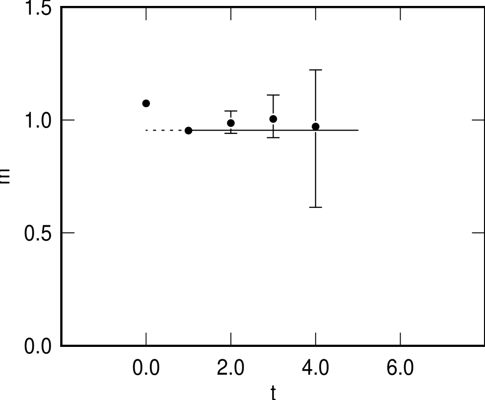
FIG. 9.: Scalar mass fit and scalar effective mass as a function of $t$ for the lattice $16^{3}\times 24$ at $\beta$ of 5.70 using the smeared operator with $n$ of 6, $\epsilon$ of 0.25 and $s$ of 2.

FIG. 10.: Scalar mass fit and scalar effective mass as a function of $t$ for the lattice $12^{3}\times 24$ at $\beta$ of 5.93 using the smeared operator with $n$ of 6, $\epsilon$ of 1.0 and $s$ of 6.

FIG. 11.: Scalar mass fit and scalar effective mass as a function of $t$ for the lattice $16^{3}\times 24$ at $\beta$ of 5.93 using the smeared operator with $n$ of 7, $\epsilon$ of 1.0 and $s$ of 5.

FIG. 12.: Scalar mass fit and scalar effective mass as a function of $t$ for the lattice $24^{3}\times 36$ at $\beta$ of 6.17 using the smeared operator with $n$ of 7, $\epsilon$ of 1.0 and $s$ of 8.

FIG. 13.: Scalar mass fit and scalar effective mass as a function of $t$ for the lattice $32^{2}\times 30\times 40$ at $\beta$ of 6.40 using the smeared operator with $n$ of 8, $\epsilon$ of 1.0 and $s$ of 10.

FIG. 14.: Tensor mass fit and tensor effective mass as a function of $t$ for the lattice $12^{3}\times 24$ at $\beta$ of 5.93 using the smeared operator with $n$ of 6, $\epsilon$ of 1.0 and $s$ of 6.

FIG. 15.: Tensor mass fit and tensor effective mass as a function of $t$ for the lattice $16^{3}\times 24$ at $\beta$ of 5.93 using the smeared operator with $n$ of 6, $\epsilon$ of 1.0 and $s$ of 5.

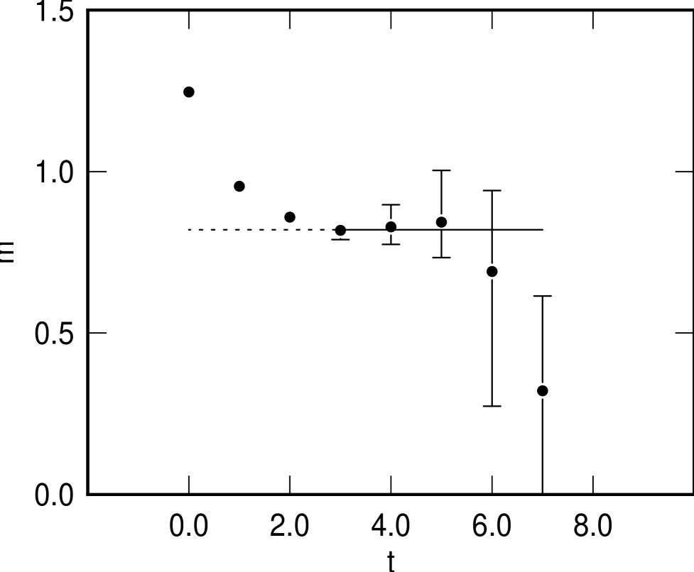
FIG. 16.: Tensor mass fit and tensor effective mass as a function of $t$ for the lattice $24^{3}\times 36$ at $\beta$ of 6.17 using the smeared operator with $n$ of 7, $\epsilon$ of 1.0 and $s$ of 9.

FIG. 17.: Tensor mass fit and tensor effective mass as a function of $t$ for the lattice $32^{2}\times 30\times 40$ at $\beta$ of 6.40 using the smeared operator with $n$ of 8, $\epsilon$ of 1.0 and $s$ of 10.

FIG. 18.: The scalar glueball mass in units of $\Lambda^{(0)}_{\overline{MS}}$ extrapolated to zero lattice spacing linearly in $[\Lambda^{(0)}_{\overline{MS}}]^{2}$.

FIG. 19.: The tensor glueball mass in units of $\Lambda^{(0)}_{\overline{MS}}$ extrapolated to zero lattice spacing linearly in $[\Lambda^{(0)}_{\overline{MS}}]^{2}$.

REFERENCES

- [1] H. Chen, J. Sexton, A. Vaccarino and D. Weingarten, Nucl. Phys. B (Proc. Suppl.) 34, 357 (1994).
- [2] D. Weingarten, Nucl. Phys. B (Proc. Suppl.) 34, 29 (1994).
- [3] J. Sexton, A. Vaccarino and D. Weingarten, Phys. Rev. Letts. 75 (1995) 4563; Nucl. Phys. B (Proc. Suppl.) 47, 128 (1996).
- [4] Don Weingarten, in Continuous Advances in QCD 1996,(edited by M. Polikarpov), World Scientific, Singapore, 1996.
- [5] W. Lee and D. Weingarten, Nucl. Phys. B (Proc. Suppl.) 73, 249 (1999).
- [6] D. H. Weingarten, Phys. Lett. 109B (1982) 57; Nucl. Phys. B215 [FS7], 1 (1983).
- [7] F. Butler, H. Chen, J. Sexton, A. Vaccarino and D. Weingarten, Phys. Rev. Letts. 70, 2849 (1993); Nucl. Phys. B430 (1994) 179; Nucl. Phys. B421, 217 (1994).
- [8] K. Kanaya, et al., Nucl. Phys. B (Proc. Suppl.) 63A-C, 161 (1998).
- [9] D. Weingarten, Nucl. Phys. B (Proc. Suppl.) 53, 232 (1997).
- [10] G. Bali, K. Schilling, A. Hulsebos, A. Irving, C. Michael, P. Stephenson, Phys. Lett. B 309, 378 (1993).
- [11] C. Morningstar and M. Peardon, Phys. Rev. D 56, 4043 (1997); hep-lat/9901004, to appear in Phys. Rev. D.
- [12] R. Gupta et al., Phys. Rev. D 43, 2301 (1993).
- [13] M. Falcioni et al., Nucl. Phys. B251, 624 (1985); M. Albanese et al., Phys. Lett. B192, 163 (1985).
- [14] M. Teper, Phys. Lett. B 183, 345 (1987).
- [15] F. R. Brown and T. J. Woch, Phys. Rev. Lett. 58, 2394 (1987).
- [16] B. Efron, The Jackknife, the Bootstrap and Other Resampling Plans, Society for Industrial and Applied Mathematics, Philadelphia, 1982.
- [17] P. van Baal and A. Kronfeld, Nucl. Phys. B (Proc. Suppl.) 9, 227 (1989).
- [18] M. Lüscher, Comm. Math. Phys. 104, 177 (1986).
- [19] G. Schierholz, Nucl. Phys. B (Proc. Suppl.) 9, 244 (1989).
- [20] G. P. Lepage and P. Mackenzie, Phys. Rev. D 48, 2250 (1993).
- [21] S. Gottlieb, private communication.
- [22] R. Sommer, Nucl. Phys. B411, 839 (1994).