Higher–Twist Contribution to Pion
Structure Function: 4–Fermi Operators

Abstract

We present quenched lattice QCD results for the contribution of higher-twist operators to the lowest non-trivial moment of the pion structure function. To be specific, we consider the combination $F_{2}^{\pi^{+}}+F_{2}^{\pi^{-}}-2F_{2}^{\pi^{0}}$ which has $I=2$ and receives contributions from 4-Fermi operators only. We introduce the basis of lattice operators. The renormalization of the operators is done perturbatively in the $\overline{\rm{MS}}$ scheme using the ’t Hooft-Veltman prescription for $\gamma_{5}$, taking particular care of mixing effects. The contribution is found to be of $O(f_{\pi}^{2}/Q^{2})$, relative to the leading contribution to the moment of $F_{2}^{\pi^{+}}$.

, , , , , , and

1 Introduction

The deviations from Bjorken scaling seen in deep-inelastic structure functions are usually interpreted as logarithmic scaling violations, as predicted by perturbative QCD. There is mounting evidence [1], however, that part of the deviations are due to power corrections induced by higher-twist effects.

This is good news: higher-twist operators probe the non-perturbative features of hadronic bound states beyond the parton model, and they may provide valuable information on the interface between perturbative and non-perturbative physics, at least in those cases where the operator product expansion (OPE) allows a clean separation between short- and long-distance phenomena.

The OPE expresses the moments of the structure function as a series of forward hadron matrix elements of local operators with coefficients decreasing as powers of $1/Q^{2}$. In general the expansion takes the form

$$M_{n}(Q^{2})=\int_{0}^{1}\mbox{d}x\,x^{n-2}F_{2}(x,Q^{2})$$ (1)

$$=C^{(2)}_{n}(Q^{2}/\mu^{2},g(\mu))\,A^{(2)}_{n}(\mu)+\frac{C^{(4)}_{n}(Q^{2}/\mu^{2},g(\mu))}{Q^{2}}\,A^{(4)}_{n}(\mu)+O\Big{(}\frac{1}{(Q^{2})^{2}}\Big{)}$$

$$\equiv M_{n}^{(2)}(Q^{2})+M_{n}^{(4)}(Q^{2})+O\Big{(}\frac{1}{(Q^{2})^{2}}\Big{)},$$

where $A(\mu)$ and $C(Q^{2}/\mu^{2},g(\mu))$ are the operator matrix elements and Wilson coefficients, respectively, renormalized at a scale $\mu$, with the superscript (2 or 4) denoting the twist. Under ideal circumstances the Wilson coefficients can be calculated perturbatively, which leaves only the matrix elements to be computed on the lattice. The leading-twist contribution can be written as

$$M_{n}^{(2)}=\sum_{f}Q_{f}^{2}\langle x_{f}^{n-1}\rangle,$$ (2)

where $x_{f}$ is the energy fraction carried by the quark of flavor $f$, and $Q_{f}$ is the charge of the quark. The higher-twist contributions usually have no parton model interpretation.

In this paper we will consider the $I=2$ pion structure function [2, 3]

$$F_{2}^{I=2}\equiv F_{2}^{\pi^{+}}+F_{2}^{\pi^{-}}-2F_{2}^{\pi^{0}}.$$ (3)

This belongs to a flavor 27-plet, is purely higher twist, and receives contributions from 4-Fermi operators only. We restrict ourselves to the lowest non-trivial moment $M_{2}$. Thus we will have to compute $A_{2}^{(4)}(\mu)$. The problem splits into two separate tasks. The first task obviously is to compute the pion matrix elements of the appropriate lattice 4-Fermi operators. The second task is to renormalize these operators at some finite scale $\mu$.

The paper is organized as follows. In sect. 2 we identify the (renormalized) operator whose matrix elements we have to compute according to the OPE. In sect. 3 we perform the renormalization of the 4-Fermi operators. This is done to 1-loop order in perturbation theory. In sect. 4 we present the results of the lattice calculation. Finally, in sect. 5 we collect our results and conclude.

2 4–Fermi Contribution

The leading twist-2 matrix element $A_{2}^{(2)}$ that enters $M_{2}$ is given by

$$\langle\vec{p}|O_{\{\mu\nu\}}|\vec{p}\rangle=2A_{2}^{(2)}[p_{\mu}p_{\nu}-\mbox{trace}],$$ (4)

$$O_{\mu\nu}=\frac{\mbox{i}}{2}\bar{\psi}\gamma_{\mu}G^{2}\overleftrightarrow{D}_{\nu}\psi-\mbox{trace},$$ (5)

where $\{\cdots\}$ means symmetrization, and $\overleftrightarrow{D}=\overrightarrow{D}-\overleftarrow{D}$. The fermion fields are 2-component vectors in flavor space, corresponding to $u$ and $d$ quarks, and the charge matrix is

$$G=\begin{pmatrix}e_{u}&0\\ 0&e_{d}\end{pmatrix}=\begin{pmatrix}2/3&0\\ 0&-1/3\end{pmatrix}.$$ (6)

The states are normalized as

$$\langle\vec{p}\,|\vec{p}\,^{\prime}\rangle=(2\pi)^{3}\,2E_{\vec{p}}\,\delta(\vec{p}-\vec{p}\,^{\prime}).$$ (7)

The Wilson coefficient has the form

$$C_{2}^{(2)}=1+O(g^{2}).$$ (8)

This contribution is the same for charged and neutral pions, and so vanishes when considering the structure function $F_{2}^{I=2}$.

The twist-4 matrix element $A_{2}^{(4)}$ receives, in general, contributions from a large variety of operators. Here we shall only be interested in 4-Fermi operators, because these are the only operators that contribute to $F_{2}^{I=2}$. Following [6, 7] we have

$$\langle\vec{p}|A^{c}_{\{\mu\nu\}}|\vec{p}\rangle=2A_{2}^{(4)}[p_{\mu}p_{\nu}-\mbox{trace}],$$ (9)

$$A^{c}_{\mu\nu}=\bar{\psi}G\gamma_{\mu}\gamma_{5}t^{a}\psi\bar{\psi}G\gamma_{\nu}\gamma_{5}t^{a}\psi-\mbox{trace}.$$ (10)

The corresponding Wilson coefficient is given by [6, 7, 8]

$$C_{2}^{(4)}=g^{2}(1+O(g^{2})).$$ (11)

The operator (10) is understood to be the renormalized, continuum operator.

3 Perturbative Renormalization

In the following we will be working in Euclidean space-time. The 4-Fermi operators that we need to consider on the lattice are

$$\begin{split}V^{c}_{\mu\nu}&=\bar{\psi}G\gamma_{\mu}t^{a}\psi\,\bar{\psi}G\gamma_{\nu}t^{a}\psi-\mbox{trace},\\[2.15277pt] A^{c}_{\mu\nu}&=\bar{\psi}G\gamma_{\mu}\gamma_{5}t^{a}\psi\,\bar{\psi}G\gamma_{\nu}\gamma_{5}t^{a}\psi-\mbox{trace},\\[2.15277pt] T^{c}_{\mu\nu}&=\bar{\psi}G\sigma_{\mu\rho}t^{a}\psi\,\bar{\psi}G\sigma_{\nu\rho}t^{a}\psi-\mbox{trace},\\[2.15277pt] V_{\mu\nu}&=\bar{\psi}G\gamma_{\mu}\psi\,\bar{\psi}G\gamma_{\nu}\psi-\mbox{trace},\\[2.15277pt] A_{\mu\nu}&=\bar{\psi}G\gamma_{\mu}\gamma_{5}\psi\,\bar{\psi}G\gamma_{\nu}\gamma_{5}\psi-\mbox{trace},\\[2.15277pt] T_{\mu\nu}&=\bar{\psi}G\sigma_{\mu\rho}\psi\,\bar{\psi}G\sigma_{\nu\rho}\psi-\mbox{trace}.\\ \end{split}$$ (12)

Summation over repeated indices and symmetrization in $\mu$, $\nu$ is understood. In our conventions $\sigma_{\mu\nu}=\frac{\rm i}{2}[\gamma_{\mu},\gamma_{\nu}]$. The $I=2$ parts of the operators are related by Fierz transformations:

$$\begin{split}V^{c}_{\mu\nu}&=-\frac{N_{c}+2}{4N_{c}}V_{\mu\nu}-\frac{1}{4}A_{\mu\nu}+\frac{1}{4}T_{\mu\nu},\\ A^{c}_{\mu\nu}&=-\frac{1}{4}V_{\mu\nu}-\frac{N_{c}+2}{4N_{c}}A_{\mu\nu}-\frac{1}{4}T_{\mu\nu},\\ T^{c}_{\mu\nu}&=\frac{1}{2}V_{\mu\nu}-\frac{1}{2}A_{\mu\nu}-\frac{1}{2N_{c}}T_{\mu\nu}.\\ \end{split}$$ (13)

The reason for considering all six operators is that they will mix under renormalization. In principle, the operators (12) could also mix with gauge variant, BRST invariant operators. But there are no such 4-Fermi operators with dimension six, and 2-Fermi operators do not contribute.

A 1-loop calculation in the continuum and on the lattice gives for the respective operator matrix elements

$$\begin{split}\langle p,p^{\prime}|O_{i}^{\rm cont}(\mu)|p,p^{\prime}\rangle&=\sum_{j}\Big{(}\delta_{ij}+\frac{g_{0}^{2}}{16\pi^{2}}R_{ij}^{\rm cont}\Big{)}\langle p,p^{\prime}|O_{j}^{\rm tree}|p,p^{\prime}\rangle,\\ \langle p,p^{\prime}|O_{i}^{\rm lat}(a)|p,p^{\prime}\rangle&=\sum_{j}\Big{(}\delta_{ij}+\frac{g_{0}^{2}}{16\pi^{2}}R_{ij}^{\rm lat}\Big{)}\langle p,p^{\prime}|O_{j}^{\rm tree}|p,p^{\prime}\rangle,\\ \end{split}$$ (14)

where $|p,p^{\prime}\rangle$ are quark states in some covariant gauge and $g_{0}$ is the bare coupling constant. The continuum matrix elements are understood to be renormalized in the $\overline{\rm{MS}}$ scheme at the scale $\mu$, while the lattice matrix elements are unrenormalized. Note that the tree-level matrix elements $\langle p,p^{\prime}|O_{j}^{\rm tree}|p,p^{\prime}\rangle$ are the same in both cases. The lattice and continuum matrix elements are then connected by

$$\begin{split}\langle p,p^{\prime}|O_{i}^{\rm cont}(\mu)|p,p^{\prime}\rangle=\sum_{j}\Big{(}\delta_{ij}-&\frac{g_{0}^{2}}{16\pi^{2}}\big{(}R_{ij}^{\rm lat}-R_{ij}^{\rm cont}\big{)}\Big{)}\\[3.01385pt] &\times\,\langle p,p^{\prime}|O_{j}^{\rm lat}(a)|p,p^{\prime}\rangle.\\ \end{split}$$ (15)

Let us write

$$\Delta R_{ij}=R_{ij}^{\rm lat}-R_{ij}^{\rm cont}.$$ (16)

While $R^{\rm lat}$ and $R^{\rm cont}$ depend on the state, $\Delta R$ is independent of the state and depends only on $a\mu$.

The renormalization constants, that take us from bare lattice to renormalized continuum numbers, are given by

$$Z_{ij}(a\mu,g)=\delta_{ij}-\frac{g_{0}^{2}}{16\pi^{2}}\Delta R_{ij}.$$ (17)

We have found it convenient to take $p=p^{\prime}$. The algebraic manipulations have been done with the help of FORM, using the ’t Hooft-Veltman prescription for dealing with the $\gamma_{5}$ matrices. This is the only prescription that has proven to give consistent results. Integrating the ’t Hooft-Veltman prescription into FORM was a non-trivial task. The algebraic workload increased by about an order of magnitude. To check the results, many of the symbolic calculations were repeated by hand. We follow the method of [9] for regularizing the infrared divergences.

The diagrams that we have calculated are shown in fig. 1. We have not made use of Fierz transformations to reduce the number of diagrams, as we could do the numerical integration fast and with high precision, and also to avoid possible problems with $d$-dimensional Fierz transformations.

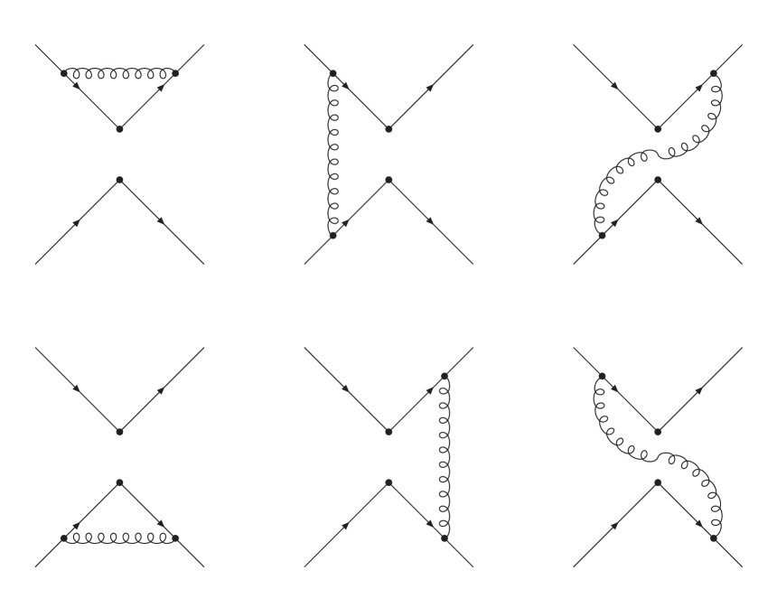
Figure 1: The 1-loop diagrams.

The 1-loop result for the renormalized 4-Fermi operators in the $\overline{\rm{MS}}$ scheme is

$$V^{c}_{\mu\nu}(\mu) = V^{c}_{\mu\nu}-\frac{g_{0}^{2}}{16\pi^{2}}\Big{[}\Big{(}-\frac{1}{2N_{c}}c_{1}+\frac{N_{c}^{2}-1}{2N_{c}}2S-N_{c}c_{2}\Big{)}V^{c}_{\mu\nu}$$

$$+ c_{4}\Big{(}\frac{N_{c}^{2}-1}{N_{c}^{2}}A_{\mu\nu}+\frac{N_{c}^{2}-4}{N_{c}}A^{c}_{\mu\nu}\Big{)}-N_{c}c_{3}T^{c}_{\mu\nu}\Big{]},$$

$$V_{\mu\nu}(\mu) = V_{\mu\nu}-\frac{g_{0}^{2}}{16\pi^{2}}\Big{[}\frac{N_{c}^{2}-1}{2N_{c}}\Big{(}c_{1}+2S\Big{)}V_{\mu\nu}+4c_{4}A^{c}_{\mu\nu}\Big{]},$$ (18)

$$A^{c}_{\mu\nu}(\mu) = A^{c}_{\mu\nu}-\frac{g_{0}^{2}}{16\pi^{2}}\Big{[}\Big{(}-\frac{1}{2N_{c}}c^{(5)}_{1}+\frac{N_{c}^{2}-1}{2N_{c}}2S-N_{c}c_{2}\Big{)}A^{c}_{\mu\nu}$$

$$+ c_{4}\Big{(}\frac{N_{c}^{2}-1}{N_{c}^{2}}V_{\mu\nu}+\frac{N_{c}^{2}-4}{N_{c}}V^{c}_{\mu\nu}\Big{)}-c_{3}\Big{(}\frac{N_{c}^{2}-1}{N_{c}^{2}}T_{\mu\nu}+\frac{N_{c}^{2}-4}{N_{c}}T^{c}_{\mu\nu}\Big{)}\Big{]},$$

$$A_{\mu\nu}(\mu) = A_{\mu\nu}-\frac{g_{0}^{2}}{16\pi^{2}}\Big{[}\frac{N_{c}^{2}-1}{2N_{c}}\Big{(}c^{(5)}_{1}+2S\Big{)}A_{\mu\nu}+4c_{4}V^{c}_{\mu\nu}-4c_{3}T^{c}_{\mu\nu}\Big{]},$$

where

$$S=\log a^{2}\mu^{2}+12.852404+(1-\alpha)\,(-\log a^{2}\mu^{2}+3.792010)$$ (19)

is the difference between the (leg) self-energy on the lattice, including the tadpole diagram, and in the continuum, and

$$\begin{split}c_{1}&=-2\log a^{2}\mu^{2}+15.530790+(1-\alpha)\,(2\log a^{2}\mu^{2}-7.584020),\\[2.15277pt] c^{(5)}_{1}&=-2\log a^{2}\mu^{2}+5.887758+(1-\alpha)\,(2\log a^{2}\mu^{2}-7.584020),\\[2.15277pt] c_{2}&=\frac{1}{2}\log a^{2}\mu^{2}-4.260157+(1-\alpha)\,(-\log a^{2}\mu^{2}+3.792010),\\[2.15277pt] c_{3}&=1.205379,\\[2.15277pt] c_{4}&=-\frac{1}{2}\log a^{2}\mu^{2}+0.094480.\\ \end{split}$$ (20)

Here $\alpha$ is the covariant gauge parameter with $\alpha=1$ corresponding to Feynman gauge and $\alpha=0$ to Landau gauge. The renormalization constants are gauge invariant. Furthermore, they are independent of $\mu$ and $\nu$, and hence of the particular representation the operators reduce to [10]. The anomalous dimensions of $V+A$ and $V^{c}+A^{c}$, which are eigenvalues of the mixing matrix, agree with the result found in [11].

Later on we will be interested in (3) for $N_{c}=3$ and $\mu=\displaystyle{1/a}$. For this case we have

$$\begin{split}V^{c}_{\mu\nu}(\mu\!=\!1/a)&=V^{c}_{\mu\nu}-g_{0}^{2}\big{(}0.281578\,\,V^{c}_{\mu\nu}+0.000532\,\,A_{\mu\nu}\\ &+0.000997\,\,A^{c}_{\mu\nu}-0.022899\,\,T^{c}_{\mu\nu}\big{)},\\[4.09024pt] V_{\mu\nu}(\mu\!=\!1/a)&=V_{\mu\nu}-g_{0}^{2}\big{(}0.348170\,\,V_{\mu\nu}+0.002393\,\,A^{c}_{\mu\nu}\big{)},\\[4.09024pt] A^{c}_{\mu\nu}(\mu\!=\!1/a)&=A^{c}_{\mu\nu}-g_{0}^{2}\big{(}0.291756\,\,A^{c}_{\mu\nu}+0.000532\,\,V_{\mu\nu}\\ &+0.000997\,\,V^{c}_{\mu\nu}-0.006785\,\,T_{\mu\nu}-0.012722\,\,T^{c}_{\mu\nu}\big{)},\\[4.09024pt] A_{\mu\nu}(\mu\!=\!1/a)&=A_{\mu\nu}-g_{0}^{2}\big{(}0.266750\,\,A_{\mu\nu}+0.002393\,\,V^{c}_{\mu\nu}\\ &-0.030533\,\,T^{c}_{\mu\nu}\big{)}.\\ \end{split}$$ (21)

Our results will be of use to other applications of 4-Fermi operators as well. For a similar calculation in the context of weak matrix elements, involving a different set of operators, see [12].

4 Lattice Calculation

4.1 General Formalism

To obtain the pion matrix elements of the operators (12), we need to compute the 3- and 2-point functions

$$\begin{split}C^{(3)}_{O}(t,\tau)&=\frac{1}{V_{S}}\langle{}^{S}\!\pi^{F}(t)\,O(\tau)\,{}^{S}\!\pi^{F^{\dagger}}(0)\rangle,\\ C^{(2)}(t)&=-\frac{1}{V_{S}}\langle{}^{S}\!\pi^{F}(t){}^{S}\!\pi^{F^{\dagger}}(0)\rangle,\\ \end{split}$$ (22)

where $V_{S}$ is the spatial volume of the lattice. The pion field is

$${}^{S}\!\pi^{F}(t)=\sum_{x;x_{4}=t}{}^{S}\!\bar{\psi}_{f\alpha}^{a}(x)F_{ff^{\prime}}(\gamma_{5})_{\alpha\beta}{}^{S}\!\psi_{f^{\prime}\beta}^{a}(x),$$ (23)

where $F$ is the flavor matrix. For the different pion states the flavor matrix takes the form

$$\begin{split}\pi^{+}&:F=\begin{pmatrix}0&1\\ 0&0\end{pmatrix},\\ \pi^{-}&:F=\begin{pmatrix}0&0\\ 1&0\end{pmatrix},\\ \pi^{0}&:F=\frac{1}{\sqrt{2}}\begin{pmatrix}1&0\\ 0&-1\end{pmatrix}.\\ \end{split}$$ (24)

The superscript $S$ in (23) denotes Jacobi-smeared quark fields:

$$\begin{split}{}^{S}\!\psi_{f\alpha}^{a}(x)&=\sum_{y;x_{4}=y_{4}=t}H^{ab}(x,y;U)\psi_{f\alpha}^{b}(y),\\ {}^{S}\!\bar{\psi}_{f\alpha}^{a}(x)&=\sum_{y;x_{4}=y_{4}=t}\bar{\psi}_{f\alpha}^{b}(y)H^{ba}(y,x;U),\\ \end{split}$$ (25)

with $H$ being given in [13], and $U$ denoting the link variables.

The 4-Fermi operators in (12) can be expressed as

$$O(\tau)=\sum_{x;\,x_{4}=\tau}\bar{\psi}_{f\alpha}^{a}(x)G_{ff^{\prime}}\Gamma_{\alpha\beta}^{ab}\,\psi_{f^{\prime}\beta}^{b}(x)\bar{\psi}_{g\gamma}^{c}(x)G_{gg^{\prime}}{\Gamma^{\prime}}_{\gamma\delta}^{\,cd}\,\psi_{g^{\prime}\delta}^{d}(x),$$ (26)

where $\Gamma$ and $\Gamma^{\prime}$ are products of $\gamma$ and $t^{a}$ matrices.

A transfer matrix calculation gives for the time dependence of the 2-point function

$$\begin{split}\langle{}^{S}\!\pi^{F}(t){}^{S}\!\pi^{F^{\dagger}}(0)\rangle&=\operatorname{Tr}[\hat{S}^{T-t}\hat{\pi}^{F}\hat{S}^{t}\hat{\pi}^{F^{\dagger}}]\\ &=\langle 0|\hat{\pi}^{F}|\pi\rangle\langle\pi|\hat{\pi}^{F^{\dagger}}|0\rangle e^{-m_{\pi}t}+\langle 0|\hat{\pi}^{F^{\dagger}}|\pi\rangle\langle\pi|\hat{\pi}^{F}|0\rangle e^{-m_{\pi}(T-t)},\\ \end{split}$$ (27)

where $|\pi\rangle$ is the pion ground state, $T$ is the time extent of the lattice, and $\hat{S}$ is the transfer matrix. All contributions from excited states have been suppressed. The pion states are normalized according to

$$\langle\pi(\vec{p})|\pi(\vec{p}\,^{\prime})\rangle=\delta_{\vec{p}\,\vec{p}\,^{\prime}}.$$ (28)

The same calculation gives for the 3-point function

$$\begin{split}\langle{}^{S}\!\pi^{F}(t)O(\tau){}^{S}\!\pi^{F^{\dagger}}(0)\rangle&=\begin{cases}\operatorname{Tr}[\hat{S}^{T-t}\hat{\pi}^{F}\hat{S}^{t-\tau}O\hat{S}^{\tau}\hat{\pi}^{F^{\dagger}}],&T\geq t\geq\tau\geq 0,\\ \operatorname{Tr}[\hat{S}^{T-\tau}O\hat{S}^{\tau-t}\hat{\pi}^{F}\hat{S}^{t}\hat{\pi}^{F^{\dagger}}],&T\geq\tau\geq t\geq 0\end{cases}\\[6.45831pt] &=\begin{cases}\langle 0|\hat{\pi}^{F}|\pi\rangle\langle\pi|O|\pi\rangle\langle\pi|\hat{\pi}^{F^{\dagger}}|0\rangle e^{-m_{\pi}t},&T\geq t\geq\tau\geq 0,\\ \langle 0|\hat{\pi}^{F^{\dagger}}|\pi\rangle\langle\pi|O|\pi\rangle\langle\pi|\hat{\pi}^{F}|0\rangle e^{-m_{\pi}(T-t)},&T\geq\tau\geq t\geq 0.\end{cases}\\ \end{split}$$ (29)

Thus for the ratio of 3- and 2-point functions we may expect to see a plateau in $\tau$ at $0\ll\tau\ll t$, and a plateau at $t\ll\tau\ll T$:

$$R_{O}(t,\tau)\equiv\frac{C^{(3)}_{O}(t,\tau)}{C^{(2)}(t)}=\begin{cases}R_{O}^{t\geqslant\tau},&0\ll\tau\ll t,\\ R_{O}^{t\leqslant\tau},&t\ll\tau\ll T,\end{cases}$$ (30)

with

$$\begin{split}R_{O}^{t\geqslant\tau}&=-\langle\pi|O|\pi\rangle\frac{e^{-m_{\pi}t}}{e^{-m_{\pi}t}+e^{-m_{\pi}(T-t)}},\\ R_{O}^{t\leqslant\tau}&=-\langle\pi|O|\pi\rangle\frac{e^{-m_{\pi}(T-t)}}{e^{-m_{\pi}t}+e^{-m_{\pi}(T-t)}}.\\ \end{split}$$ (31)

The sum is independent of $t$, and finally we obtain

$$\langle\pi|O|\pi\rangle=-R_{O}^{t\geqslant\tau}-R_{O}^{t\leqslant\tau}.$$ (32)

4.2 Technical Details

We will now re-write the 3-point function (22) in terms of quark propagators. Two different kinds of propagators are emerging, depending on whether we start from a smeared quark field and end on a local one, or vice versa. The local-smeared and smeared-local propagators, ${}^{SL}\!\Delta$ and ${}^{LS}\!\Delta$, are given by

$$\begin{split}\langle{}^{S}\!\psi_{f\alpha}^{a}(x)\bar{\psi}_{f^{\prime}\beta}^{b}(y)\rangle_{\bar{\psi},\psi}&=\delta_{ff^{\prime}}{}^{SL}\!\Delta_{\alpha\beta}^{ab}(x,y)\\ \langle\psi_{f\alpha}^{a}(x){}^{S}\!\bar{\psi}_{f^{\prime}\beta}^{b}(y)\rangle_{\bar{\psi},\psi}&=\delta_{ff^{\prime}}{}^{LS}\!\Delta_{\alpha\beta}^{ab}(x,y),\end{split}$$ (33)

with

$${}^{LS}\!\Delta(x,y)=\gamma_{5}{}^{SL}\!\Delta(y,x)^{\dagger}\gamma_{5}.$$ (34)

(We have suppressed the dependence on $U$.)

For $I=2$, and after having summed over flavor indices, we obtain

$$C^{(3)}_{O}(t,\tau) = (e_{u}-e_{d})^{2}\frac{1}{V_{S}}\sum_{x;\,x_{4}=t}\sum_{y;\,y_{4}=\tau}\sum_{z;\,z_{4}=0}\big{\{}$$

$$\langle\,\operatorname{Tr}[{}^{LS}\!\Delta(y,z)\gamma_{5}{}^{SL}\!\Delta(z,y)\Gamma^{\prime}{}^{LS}\!\Delta(y,x)\gamma_{5}{}^{SL}\!\Delta(x,y)\Gamma]\,\rangle_{U}$$

$$+ \langle\,\operatorname{Tr}[{}^{LS}\!\Delta(y,z)\gamma_{5}{}^{SL}\!\Delta(z,y)\Gamma{}^{LS}\!\Delta(y,x)\gamma_{5}{}^{SL}\!\Delta(x,y)\Gamma^{\prime}]\,\rangle_{U}$$

$$- \langle\,\operatorname{Tr}[{}^{LS}\!\Delta(y,z)\gamma_{5}{}^{SL}\!\Delta(z,y)\Gamma^{\prime}]\operatorname{Tr}[{}^{LS}\!\Delta(y,x)\gamma_{5}{}^{SL}\!\Delta(x,y)\Gamma]\,\rangle_{U}$$

$$- \langle\,\operatorname{Tr}[{}^{LS}\!\Delta(y,z)\gamma_{5}{}^{SL}\!\Delta(z,y)\Gamma]\operatorname{Tr}[{}^{LS}\!\Delta(y,x)\gamma_{5}{}^{SL}\!\Delta(x,y)\Gamma^{\prime}]\,\rangle_{U}\big{\}}.$$

One of the spatial sums can be eliminated by making use of translational invariance, finally giving

$$C^{(3)}_{O}(t,\tau) = (e_{u}-e_{d})^{2}\sum_{x;\,x_{4}=t-\tau}\sum_{z;\,z_{4}=-\tau}\big{\{}$$

$$\langle\,\operatorname{Tr}[{}^{LS}\!\Delta(0,z)\gamma_{5}{}^{SL}\!\Delta(z,0)\Gamma^{\prime}{}^{LS}\!\Delta(0,x)\gamma_{5}{}^{SL}\!\Delta(x,0)\Gamma]\,\rangle_{U}$$

$$+ \langle\,\operatorname{Tr}[{}^{LS}\!\Delta(0,z)\gamma_{5}{}^{SL}\!\Delta(z,0)\Gamma{}^{LS}\!\Delta(0,x)\gamma_{5}{}^{SL}\!\Delta(x,0)\Gamma^{\prime}]\,\rangle_{U}$$

$$- \langle\,\operatorname{Tr}[{}^{LS}\!\Delta(0,z)\gamma_{5}{}^{SL}\!\Delta(z,0)\Gamma^{\prime}]\operatorname{Tr}[{}^{LS}\!\Delta(0,x)\gamma_{5}{}^{SL}\!\Delta(x,0)\Gamma]\,\rangle_{U}$$

$$- \langle\,\operatorname{Tr}[{}^{LS}\!\Delta(0,z)\gamma_{5}{}^{SL}\!\Delta(z,0)\Gamma]\operatorname{Tr}[{}^{LS}\!\Delta(0,x)\gamma_{5}{}^{SL}\!\Delta(x,0)\Gamma^{\prime}]\,\rangle_{U}\big{\}}.$$

All 3-point functions can be built from

$$Q_{\alpha\beta}^{ab}(t)=\sum_{x;\,x_{4}=t}{}^{LS}\!\Delta_{\alpha\gamma}^{ac}(0,x)(\gamma_{5})_{\gamma\delta}{}^{SL}\!\Delta_{\delta\beta}^{cb}(x,0),$$ (37)

where the first propagator can be obtained from the second one by means of (34). In terms of (37) the 3-point function reads

$$\begin{split}C^{(3)}_{O}(t,\tau)&=(e_{u}-e_{d})^{2}\big{\{}\langle\,\operatorname{Tr}[Q(-\tau)\Gamma^{\prime}Q(t-\tau)\Gamma]\,\rangle_{U}\\ &+\langle\operatorname{Tr}[Q(-\tau)\Gamma Q(t-\tau)\Gamma^{\prime}]\,\rangle_{U}\\ &-\langle\,\operatorname{Tr}[Q(-\tau)\Gamma^{\prime}]\operatorname{Tr}[Q(t-\tau)\Gamma]\,\rangle_{U}\\ &-\langle\,\operatorname{Tr}[Q(-\tau)\Gamma]\operatorname{Tr}[Q(t-\tau)\Gamma^{\prime}]\,\rangle_{U}\big{\}}.\\ \end{split}$$ (38)

Figure 2: The ratio R for the $44$-component of the operator $A$ at $t=10$, 16 and 22 for $\kappa=0.1515$. The fit intervals and the results of the fit are shown by the dashed lines.

By computing the propagators from a local source at $t=0$ to all $t<T$ using sink-smearing we obtain the 3-point functions for all $t$ and $\tau$.

4.3 Results of the Simulation

The numerical calculations are done on a $16^{3}\times 32$ lattice at $\beta\equiv 6/g_{0}^{2}=6.0$ in the quenched approximation. We use Wilson fermions. To be able to extrapolate our results to the chiral limit, the calculations are done at three values of the hopping parameter, $\kappa=0.1550$, 0.1530 and 0.1515. This corresponds to physical quark masses of about 70, 130 and 190 MeV, respectively. For the gauge update we use a 3-hit Metropolis sweep followed by 16 overrelaxation sweeps, and we repeat this 50 times to generate a new configuration. Our data sample consists of 400 configurations.

In the following we shall restrict ourselves to zero momentum pion states and operators with $\mu=\nu=4$. In fig. 2 we show the ratio (30) for the operator $A$ at three different values of $t$. We find very good plateaus in $\tau$. In our final fits we have averaged over $t$ values around $T/2$.

To obtain continuum results we have to multiply each quark field by $\sqrt{2\kappa}$, and a factor of $2m_{\pi}$ is needed to convert to the continuum normalization of states:

$$\langle\pi|O|\pi\rangle^{\rm cont}=(2\kappa)^{2}\,2m_{\pi}\,\langle\pi|O|\pi\rangle^{\rm lat}.$$ (39)

For the reduced matrix element $A_{2}^{(4)}$ (in (9)) we then find

$$A_{2}^{(4)}=\frac{4}{3}\,\frac{(2\kappa)^{2}}{m_{\pi}}\,\langle\pi|A^{c}_{44}|\pi\rangle^{\rm lat},\;\langle\pi|A^{c}_{44}|\pi\rangle^{\rm lat}=-R_{A^{c}_{44}}^{t\geqslant\tau}-R_{A^{c}_{44}}^{t\leqslant\tau},$$ (40)

where $A^{c}_{44}$ is the renormalized operator, as given in (3).

$\kappa$	$af_{\pi B}$	$am_{\pi}$
0.1515	0.122(2)	0.5037(8)
0.1530	0.113(2)	0.4237(8)
0.1550	0.098(2)	0.3009(10)

Table 1: Pion masses and unrenormalized (bare) decay constants.

$\bar{O}$	$\kappa$			Chiral Limit
	$\;0.1515$	$\;0.1530$	$\;0.1550$	$\kappa_{c}=0.15717$	$\;\;\chi^{2}$
$\bar{A}\,f^{-2}_{\pi B}$	0.561(13)	0.546(17)	0.514(25)	0.490(37)	0.0593
$\bar{V}\,f^{-2}_{\pi B}$	-0.139(9)	-0.154(13)	-0.212(23)	-0.237(31)	0.897
$\bar{T}\,f^{-2}_{\pi B}$	-0.207(21)	-0.200(30)	-0.197(47)	-0.190(67)	0.00397
$\bar{A}^{c}\,f^{-2}_{\pi B}$	-0.147(11)	-0.139(16)	-0.111(27)	-0.098(38)	0.111
$\bar{V}^{c}\,f^{-2}_{\pi B}$	-0.134(12)	-0.122(17)	-0.089(29)	-0.071(40)	0.113
$\bar{T}^{c}\,f^{-2}_{\pi B}$	-0.315(30)	-0.317(43)	-0.330(68)	-0.334(96)	0.00880

Table 2: The unrenormalized, reduced matrix elements $\bar{O}$, together with their extrapolations to the chiral limit.

The lattice pion masses are given in table 1. In the following we shall express the dimensionful matrix elements in terms of the pion decay constant $f_{\pi}$, whose unrenormalized values are also given in the table. The pion masses and the decay constants are taken from [14], where we had a slightly higher statistics.

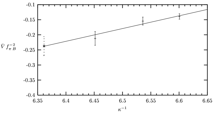
Figure 3: The unrenormalized, reduced matrix elements $\bar{A}$, $\bar{V}$ and $\bar{T}$, and their extrapolations to the chiral limit.

Figure 4: The unrenormalized, reduced matrix elements $\bar{A}^{c}$, $\bar{V}^{c}$ and $\bar{T}^{c}$, and their extrapolations to the chiral limit.

In table 2 we give our results for the unrenormalized, reduced matrix elements $\bar{O}=-((2\kappa)^{2}/m_{\pi})\,\langle\pi|O_{44}|\pi\rangle^{\rm lat}$ of the various $I=2$ operators. The reader can easily check that the Fierz identities (13) hold identically at each value of $\kappa$. In fig. 3 we plot $\bar{O}$ for the operators without color matrices, and in fig. 4 for the operators with color matrices, as a function of $\kappa^{-1}$. The data suggest a linear extrapolation to the chiral limit. The result of the extrapolation is given in table 2. The critical hopping parameter is $\kappa_{c}=0.15717(3)$.

5 Results and Conclusions

We are now ready to give results for the structure function. To minimize effects of higher order contributions to the Wilson coefficient $C_{2}^{(4)}$ in $g^{2}$, we shall take

$$Q^{2}=\mu^{2}=a^{-2}.$$ (41)

The $g^{2}$ in (11) is therefore replaced by $4\pi\alpha_{s}(Q^{2})$. If we fix the scale by adjusting the $\rho$ mass to its physical value, we have [14] $a^{-2}\approx 5\,\mbox{GeV}^{2}$. If, instead, we take the string tension or the force parameter to set the scale, we have $a^{-2}\approx 4\,\mbox{GeV}^{2}$.

We calculate the renormalization constants from (21) with $g_{0}=1$. Combining these with the unrenormalized lattice results in table 2, we find for the $I=2$ structure function

$$A_{2}^{(4)\,I=2}=0.100(38)\,f^{\,2}_{\pi B}.$$ (42)

Multiplying this number with the Wilson coefficient and the kinematical factor, and expressing the result in terms of the renormalized decay constant $f_{\pi}=Z_{A}f_{\pi B}$ with $Z_{A}=0.867$, computed in perturbation theory, we finally obtain

$$M_{2}^{I=2}=1.67(64)\,\frac{f_{\pi}^{2}\,\alpha_{s}(Q^{2})}{Q^{2}}+O(\alpha_{s}^{2}).$$ (43)

All numbers refer to the chiral limit. An early calculation [3], based on 15 configurations, found a negative value for $M_{2}^{I=2}$.

It is instructive to compare (43) with the twist-2 contribution to the structure function of (say) the $\pi^{+}$. In [13] we found

$$M_{2}^{(2)\,\pi^{+}}=0.152(7).$$ (44)

Relative to this number (43) is only a small correction, except perhaps at very small values of $Q^{2}$.

In case of the nucleon we may expect similar numbers, but with $f_{\pi}$ being replaced by the nucleon mass. This would then result in a significant correction. Calculations of 4-Fermi contributions to the nucleon structure function are in progress.

References

- [1] S. Liuti, Nucl. Phys. B (Proc. Suppl.) 74 (1999) 380 (hep-ph/9809248).
- [2] S. Gottlieb, Nucl. Phys. B139 (1978) 125.
- [3] A. Morelli, Nucl. Phys. B392 (1993) 518.
- [4] S. Capitani, M. Göckeler, R. Horsley, H. Oelrich, D. Petters, P. Rakow and G. Schierholz, Nucl. Phys. B (Proc. Suppl.) 73 (1999) 288 (hep-lat/9809171).
- [5] S. Capitani, M. Göckeler, R. Horsley, D. Petters, D. Pleiter, P. Rakow, G. Schierholz, DESY preprint DESY 99-069 (hep-ph/9906320).
- [6] R. L. Jaffe and M. Soldate, Phys. Lett. 105B (1981) 467.
- [7] R. L. Jaffe and M. Soldate, Phys. Rev. D26 (1982) 49.
- [8] E. V. Shuryak and A. I. Vainshtein, Nucl. Phys. B199 (1982) 451.
- [9] H. Kawai, R. Nakayama and K. Seo, Nucl. Phys. B189 (1981) 40.
- [10] M. Göckeler, R. Horsley, E.-M. Ilgenfritz, H. Perlt, P. Rakow, G. Schierholz and A. Schiller, Phys. Rev. D54 (1996) 5705.
- [11] M. Okawa, Nucl. Phys. B187 (1981) 71.
- [12] M. Gupta, T. Bhattacharya and S. R. Sharpe, Phys. Rev. D55 (1997) 4036.
- [13] C. Best, M. Göckeler, R. Horsley, E.-M. Ilgenfritz, H. Perlt, P. Rakow, A. Schäfer, G. Schierholz, A. Schiller and S. Schramm, Phys. Rev. D56 (1997) 2743.
- [14] M. Göckeler, R. Horsley, H. Perlt, P. Rakow, G. Schierholz, A. Schiller and P. Stephenson, Phys. Rev. D57 (1998) 5562.