Heavy Quark Potentials in Quenched QCD at High Temperature

Abstract

Heavy quark potentials are investigated at high temperatures. The temperature range covered by the analysis extends from $T$ values just below the deconfinement temperature up to about $4T_{c}$ in the deconfined phase. We simulated the pure gauge sector of QCD on lattices with temporal extents of 4, 6 and 8 with spatial volumes of $32^{3}$. On the smallest lattice a tree level improved action was employed while in the other two cases the standard Wilson action was used. Below $T_{c}$ we find a temperature dependent logarithmic term contributing to the confinement potential and observe a string tension which decreases with rising temperature but retains a finite value at the deconfinement transition. Above $T_{c}$ the potential is Debye-screened, however simple perturbative predictions do not apply.

PACS-Indices : 5.70.Ce 12.38.Gc 12.39.Pn

Keywords : Static quark potential, Finite temperature, Debye screening

1 Introduction

The static quark potential at high temperatures is interesting for several reasons. Phenomenologically, the properties of quark bound states, in particular of heavy quarkonia, can be derived from potential models quite successfully. It is then important to compute the temperature dependence of the potential as this might lead to observable consequences in heavy ion collision experiments. Notably, it has been suggested to use the suppression of $J/\Psi$ and $\Psi^{\prime}$ production [1] as a signal for the quark-gluon plasma. For this purpose, a detailed knowledge of the temperature dependence of the potential appears very helpful [2].

Moreover, it is well known that a linearly increasing potential at large distances arises naturally from a string picture of confinement. As long as one stays in the confined phase of QCD, string models then also predict a definite behaviour of the potential at finite temperatures [3, 4, 5]. These predictions ought to be tested by lattice analyses.

In close vicinity of the deconfinement transition temperature the static quark potential and the mass gap i.e. the potential integrated over perpendicular directions are sensitive to the order of the phase transition. In colour $SU(3)$ the observation of a finite mass gap at the critical temperature supported that the transition is of first order [6], while in $SU(2)$ a continuous decrease to zero with the appropriate Ising critical exponents was found [7].

In the deconfined phase, asymptotic freedom suggests that at high temperatures the plasma consists of weakly interacting quarks and gluons. Previous numerical studies [8-12] have, however, shown that non-perturbative phenomena prevail up to temperatures of at least several times the critical temperature. In particular, the heavy quark potential did not show the simple Debye-screened behaviour anticipated from a resummed lowest-order perturbative treatment [13]. This might not be too surprising as various non-perturbative modes may play a role in the long distance sector of the plasma [14]. It is then important to quantify colour screening effects by a genuinely non-perturbative approach.

In the present paper we compute the static quark potential in the pure gluonic sector of QCD. We investigate the temperature dependence of the potential over a range of temperatures from 0.8 to about 4 times the critical temperature $T_{c}$. The analysis is based on gluon configurations generated on lattices of size $32^{3}\times N_{\tau}$ with $N_{\tau}=4,6$ and $8$. This enables us to gain some control over finite lattice spacing artefacts. On the smallest lattice a tree level improved gauge action was used while on the two bigger lattices a standard Wilson action was employed. We go beyond previous studies of the potential in so far the temperature range is covered more densely and also because a large set of lattice distances was probed. This helps to extract fit parameters with higher reliability.

The paper is organized such that the next section summarizes theoretical expectations on the behaviour of the potential both below and above the transition temperature. In section 3 we present and discuss our results for the potential in the confined phase. Section 4 contains our findings for temperatures above $T_{c}$ and section 5 the conclusion.

2 Theoretical Expectations

Throughout this paper the potential is computed from Polyakov loop correlations

$$\langle L({\vec{0}})L^{\dagger}({\vec{R}})\rangle=\exp\{-V(|{\vec{R}}|,T)/T\}$$ (1)

where

$$L({\vec{x}})=\frac{1}{3}{\rm tr}\prod_{\tau=1}^{N_{\tau}}U_{0}({\vec{x}},\tau)$$ (2)

denotes the Polyakov loop at spatial coordinates ${\vec{x}}$. In the limit $R\rightarrow\infty$ the correlation function should approach the cluster value $|\langle L(0)\rangle|^{2}$ which vanishes if the potential is rising to infinity at large distances (confinement) and which acquires a finite value in the deconfined phase.

In the limit where the flux tube between two static quarks can be considered as a string, predictions about the behaviour of the potential are available from computations of the leading terms arising in string models. For zero temperature one expects

$$V(R)=V_{0}-\frac{\pi}{12}\frac{1}{R}+\sigma R$$ (3)

where $V_{0}$ denotes the self energy of the quark lines, $\sigma$ is the string tension and the Coulomb-like $1/R$ term stems from fluctuations of the string [15]. Eq. (3) generally gives a good description of the zero temperature ground-state potential although it has been shown [16] that the excitation spectrum meets string model predictions only at large quark pair separations. For non-vanishing temperatures below the critical temperature of the transition to deconfinement, a temperature-dependent potential has been computed [5] as

$$V(R,T) = V_{0}-\left[\frac{\pi}{12}-\frac{1}{6}{\rm arctan}(2RT)\right]\frac{1}{R}$$ (4)

$$\mbox{}+\left[\sigma-\frac{\pi}{3}T^{2}+\frac{2}{3}T^{2}{\rm arctan}(\frac{1}{2RT})\right]R+\frac{T}{2}\ln(1+(2RT)^{2})$$

In the limit $R\gg 1/T$ this goes over into

$$V(R,T)=V_{0}+\left[\sigma-\frac{\pi}{3}T^{2}\right]R+T\ln(2RT)$$ (5)

which had been calculated previously [4]. Note the logarithmic term which originates from transverse momentum fluctuations. So far, it has been left open whether the string tension $\sigma$ appearing in eqs. (4) and (5) is identical to the zero temperature value. In the context of a low temperature or large $R$ expansion, the temperature dependent terms appearing in eqs. (4) and (5) should, however, be considered as thermal corrections to the zero temperature string tension. An explicitly temperature-dependent string tension was computed by means of a $1/D$ expansion [3]

$$\frac{\sigma(T)}{\sigma(0)}=\sqrt{1-\frac{T^{2}}{T_{c}^{2}}}$$ (6)

where $T_{c}$ was obtained as

$$T_{c}^{2}=\frac{3}{\pi(D-2)}\sigma(0)\quad.$$ (7)

Note, however, that for $D\rightarrow\infty$ the phase transition is of second order leading to a continuous vanishing of the string tension at the deconfinement temperature. In colour $SU(2)$, which also exhibits a second order transition, it was established [7] that $\sigma(T)$ vanishes $\sim(\beta_{c}-\beta)^{\nu}$ with a critical exponent $\nu$ taking its 3-D Ising value of 0.63 as suggested by universality. In the present case of colour $SU(3)$ one expects a discontinuous behaviour and a non-vanishing string tension at the critical temperature.

In the deconfined phase the Polyakov loop acquires a non-zero value. Thus, we can normalize the correlation function to the cluster value $|\langle L\rangle|^{2}$, thereby removing the quark-line self energy contributions. Moreover, the quark-antiquark pair can be in either a colour singlet or a colour octet state. Since in the plasma phase quarks are deconfined the octet contribution does not vanish and the Polyakov loop correlation is a colour-averaged mixture of both

$$e^{-V(R,T)/T}=\frac{1}{9}e^{-V_{1}(R,T)/T}+\frac{8}{9}e^{-V_{8}(R,T)/T}$$ (8)

At high temperatures, perturbation theory predicts [13] that $V_{1}$ and $V_{8}$ are related as

$$V_{1}=-8V_{8}+{\cal O}(g^{4})$$ (9)

Correspondingly, the colour-averaged potential is given by

$$\frac{V(R,T)}{T}=-\frac{1}{16}\frac{V_{1}^{2}(R,T)}{T^{2}}$$ (10)

Due to the interaction with the heat bath the gluon acquires a chromo-electric mass $m_{e}(T)$ as the IR limit of the vacuum polarization tensor. To lowest order in perturbation theory, this is obtained as

$$\left(\frac{m_{e}^{(0)}(T)}{T}\right)^{2}=g^{2}(T)\left(\frac{N_{c}}{3}+\frac{N_{F}}{6}\right)$$ (11)

where $g(T)$ denotes the temperature-dependent renormalized coupling, $N_{c}$ is the number of colours and $N_{F}$ the number of quark flavours. The electric mass is also known in next-to-leading order [17] in which it depends on an anticipated chromo-magnetic gluon mass although the magnetic gluon mass itself cannot be calculated perturbatively. Fourier transformation of the gluon propagator leads to the Debye-screened Coulomb potential for the singlet channel

$$V_{1}(R,T)=-\frac{\alpha(T)}{R}e^{-m_{e}(T)R}$$ (12)

where $\alpha(T)=g^{2}(T)(N_{c}^{2}-1)/(8\pi N_{c})$ is the renormalized T-dependent fine structure constant. It has been stressed [18] that eq. (12) holds only in the IR limit $R\rightarrow\infty$ because momentum dependent contributions to the vacuum polarization tensor have been neglected. Moreover, at temperatures just above $T_{c}$ perturbative arguments will not apply so that we have chosen to attempt a parametrization of the numerical data with the more general ansatz [10]

$$\frac{V(R,T)}{T}=-\frac{e(T)}{(RT)^{d}}e^{-\mu(T)R}$$ (13)

with an arbitrary power $d$ of the $1/R$ term, an arbitrary coefficient $e(T)$ and a simple exponential decay determined by a general screening mass $\mu(T)$. Only for $T\gg T_{c}$ and large distances we expect that $d\rightarrow 2$ and $\mu(T)\rightarrow 2m_{e}(T)$, eq. (10), corresponding to two-gluon exchange.

3 Results below $T_{c}$

The results to be presented here as well as in the next section are based on two different sets of data. The first set, referred to as (I) in the following, was generated with a tree-level Symanzik-improved gauge action consisting of $1\times 1$ and $2\times 1$ loops. The lattice size was $32^{3}\times 4$. We used a pseudo-heatbath algorithm [20] with FHKP updating [21] in the $SU(2)$ subgroups. Each heatbath iteration is supplemented by 4 overrelaxation steps [22]. To improve the signal in calculations of Polyakov loop correlation functions link integration [23] was employed. For each $\beta$-value the data set consists of 20000 to 30000 measurements separated by one sweep.

The second set of data (II) was obtained as a by-product of earlier work, the analysis of the equation of state [19]. The gauge configurations used in the present study were generated with the standard Wilson gauge action on lattices of size $32^{3}\times 6$ and $32^{3}\times 8$. The same algorithm as for (I) was employed. The statistics amounts to 1000 to 4000 measurements separated by 10 sweeps for the $N_{\tau}=6$ data and between 15000 and 30000 measurements at each sweep for $N_{\tau}=8$. The errors on the potentials as well as the fit parameters were determined by jackknife in both cases.

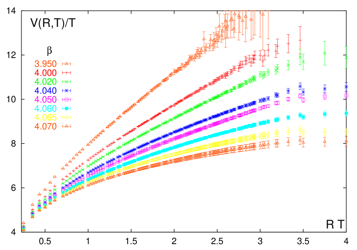
Figure 1: The potentials in units set by the temperature at the $\beta$ values analyzed for $N_{\tau}=4$ (case I). The critical coupling for this action on our lattice size has been determined as $\beta_{c}=4.0729(3)$ [24].

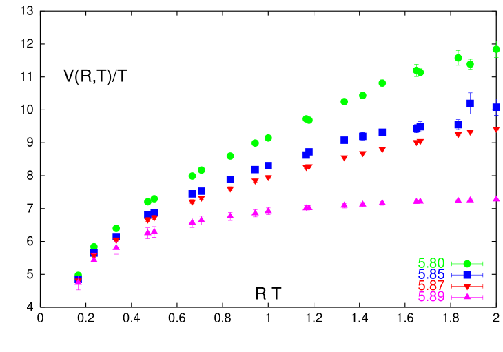
Figure 2: The same as figure 1 except for $N_{\tau}=6$ (case II). The critical coupling is $\beta_{c}=5.8938(11)$ [19].

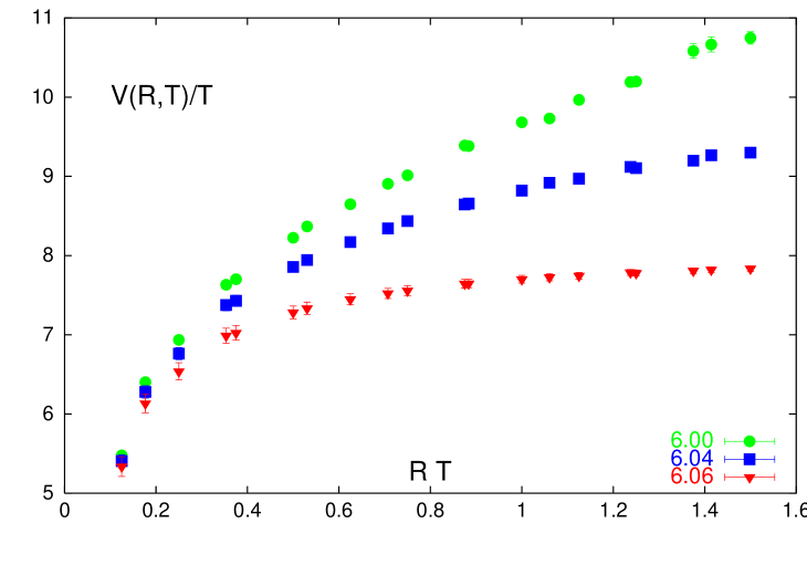
Figure 3: The same as figure 1 except for $N_{\tau}=8$ (case II). The critical coupling is $\beta_{c}=6.0609(9)$ [19].

The lattice results for the potential at temperatures below $T_{c}$ are shown in Figures 1, 2 and 3. The correlation functions, eq. (1), have been computed not only for on-axis separations but also for some, in the case I almost all, off-axis distance vectors $\vec{R}$. Although the lattice spacing for the $N_{\tau}=4$ data is larger than for the other two lattice sizes rotational symmetry is quite well satisfied due to the use of an improved action in this case. As we will focus on the intermediate to large distance behaviour of the potential, it was not attempted to specifically treat the deviations from rotational invariance at small separations. Note that the distances covered by the data extend to $RT\raise 1.29167pt\hbox{$<$\kern-7.5pt\raise-4.73611pt\hbox{$\sim$}}4$ for (I) while in case II we could obtain signals up to $RT\,\raise 1.29167pt\hbox{$<$\kern-7.5pt\raise-4.73611pt\hbox{$\sim$}}\,2$.

The potentials have first been fitted to eq. (4) with two free parameters, the self-energy $V_{0}$ and a possibly temperature-dependent string tension $\sigma(T)$. These fits work rather well even when data at small separations are included because the fit ansatz also accounts for a $1/R$ piece in the potential. The results to be quoted for the string tension, Table 1, have, however, been obtained when the data at small separations are excluded from the fit. Typically, a minimal distance of $RT\simeq 1/2$ was chosen. The fits are stable under variation of $R_{\rm min}$ in this ballpark and return good $\raise 1.72218pt\hbox{$\chi$}^{2}$ values. Varying the maximum distance to be fitted does not lead to noticeable changes of the results. This holds for all three lattices.

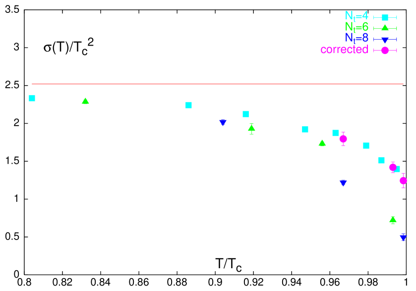
Figure 4: The string tension at non-vanishing temperature as obtained from fits with eq. (4). The line denotes the zero temperature string tension. In both cases the string tension was normalized to $T_{c}$. For an explanation of the ‘corrected’ data points see text.

The results for the string tension, normalized to the critical temperature squared, $\sigma/T_{c}^{2}$, are summarized in Figure 4. The temperature scale has been determined from measurements of the string tension at $T=0$ [19, 25, 26]. The finite temperature string tension is compared to these results at zero temperature, $\sigma(0)/T_{c}^{2}$, shown as the line in the figure. Quite clearly, in the investigated temperature range there are substantial deviations from the zero temperature string tension. These deviations amount to about 10 % at $T/T_{c}=0.8$ and become larger when the temperature is raised.

Close to $T_{c}$ the results from $N_{\tau}=6$ and $8$ at first sight do not seem to agree with the numbers coming from the $N_{\tau}=4$ lattices. However, recall that the $SU(3)$ quenched theory exhibits a first order transition with the coexistence of hadron and plasma phase at the critical temperature. The tunneling rate between the two phases decreases exponentially $\sim\exp(-2\hat{\sigma}\times(N_{\sigma}/N_{\tau})^{2})$ where $\hat{\sigma}=\sigma_{I}/T_{c}^{3}$ is the normalized interface tension. The lattices of data set (II) have a smaller aspect ratio of $N_{\sigma}/N_{\tau}=4$ and 5.33, respectively, than the $N_{\tau}=4$ lattice whose aspect ratio is 8. Correspondingly, the ensemble of configurations of the second set contains (more) configurations in the “wrong”, the deconfined phase. In fact, close to $T_{c}$, Polyakov loop histograms reveal this two-state distribution for $N_{\tau}=6$ and 8, with a clear separability between the two Gaussian-like peaks. Such a two-state signal is absent for the $N_{\tau}=4$ data. Carrying out the averaging of the potential only over configurations with Polyakov loops in the confined peak leads to the corrected data points in Figure 4. At temperatures not so close to $T_{c}$ this separation of phases is not possible anymore as the Polyakov loop histogram has tails into the deconfined phase but it is not clear where one should set the cut.

When we apply this correction the agreement of the results from the three different lattices is evident. This shows that the temperature dependence of the string tension is not subject to severe discretisation effects. Moreover, the functional form of the fit ansatz eq. (4), as suggested by string model calculations, describes the behaviour of the lattice data quite well. However, with increasing temperature we observe a substantial decrease of the string tension away from its zero temperature value. Since the fit ansatz, eq. (4), contains already a $\pi/3\ast T^{2}$ term, the decreasing slope of the linear part of the potential can not solely be accounted for by this leading correction.

In order to analyze the linear rising part of the potential in a more model-independent way, in a second round of fits we have compared our data with the ansatz

$$V(R,T)=V_{0}+\sigma(T)R+CT\ln(2RT)$$ (14)

Note that this ansatz differs from eq. (5) in so far it summarizes all the linear dependence on the distance $R$ by an explicitly temperature dependent string tension $\sigma(T)$. Due to its lacking of a $1/R$ piece this formula is very well capable of describing the data but only if the fit is applied to large distances of $RT\geq 1$. For data set (II) this requirement leaves not too many data points to be fitted. In this case we checked that eq. (14) is able to parametrize the potential. However, since we do not have as much room to check for stability of the results as one would wish, we refrain from quoting results for data set (II). In case I we do have enough distances and obtain fits with good $\raise 1.72218pt\hbox{$\chi$}^{2}$ values which are stable under variation of the minimal distance to be included in the minimization.

On data set (I) we clearly observe the logarithmic term contained in eqs. (5) and (14). The fits return values for the coefficient $C$ of the logarithm which are equal to 1 within an error margin of less than 10 %. We thus confirm a logarithmic piece in the potential with a strength as anticipated from the string model calculation [4] or, equivalently, a subleading power-like $1/R$-factor with power 1 contributing to the Polyakov-loop correlation function.

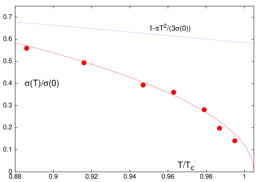
Figure 5: The string tension as obtained from fits with eq. (14), normalized to its zero temperature value. The line is the result of a fit to this ratio with the string model motivated ansatz eq. (15). The data is compared with the lowest order temperature effect on the linear part of the potential, eq. (5), shown as the dotted line.

Because of these findings, we fix this coefficient to 1 in the following. The resulting string tension, normalized to its zero temperature value is shown in Figure 5. The temperature dependence compares well with the (modified) prediction [3] of the Nambu-Goto model, eq. (6),

$$\frac{\sigma(T)}{\sigma(0)}=a\sqrt{1-b\frac{T^{2}}{T_{c}^{2}}}$$ (15)

Recall that the string model prediction assumes a second order transition with a continuous vanishing of the string tension at the critical temperature. The deconfinement transition in pure $SU(3)$ Yang-Mills theory, however, is known to be of first order. Thus, a discontinuity at the critical temperature is expected. To account for this, the coefficients $a$ and $b$ in eq. (15) are allowed to deviate from unity. In fact, the fit to the data, shown as the line in figure 5, results in the values $a=1.21(5)$ and $b=0.990(5)$. This leads to a non-vanishing string tension at the critical temperature of

$$\frac{\sigma(T_{c})}{\sigma(0)}=0.121(35)$$ (16)

This number can be converted into a value for the (physical) mass gap at the transition point, $m_{\rm phys}(T_{c})/T_{c}=\sigma(T_{c})/T_{c}^{2}=0.30(9)$. This is a bit below but not incompatible with earlier results of dedicated analyses of the order of the deconfinement transition, $m_{\rm phys}(T_{c})/T_{c}=0.4-0.8$, as summarized in [6].

Finally, we compared the string tension $\sigma(T)$ defined in eq. (14) with the leading behaviour $\sigma(0)-\pi T^{2}/3$ as given in eq. (5). This is shown as the dotted line in Figure 5. Similarly to Figure 4 the comparison fails, reflecting that non-leading terms contribute substantially.

4 Results above $T_{c}$

Above the critical temperature we have normalized the Polyakov loop correlations to their cluster value

$$V(|\vec{R}|,T)=-T\ln\frac{\langle L(0)L^{\dagger}(\vec{R})\rangle}{|\langle L(0)\rangle|^{2}}$$ (17)

to eliminate the self-energy contributions. In principle, the correlation function itself is periodic in $R$. Alternatively, one can fit the potential, eq. (17), with a periodic ansatz, $V(R)\rightarrow V(R)+V(N_{\sigma}a-R)$. The second contribution turns out to be very small at the distances fitted and both procedures lead to the same results for the fit parameters.

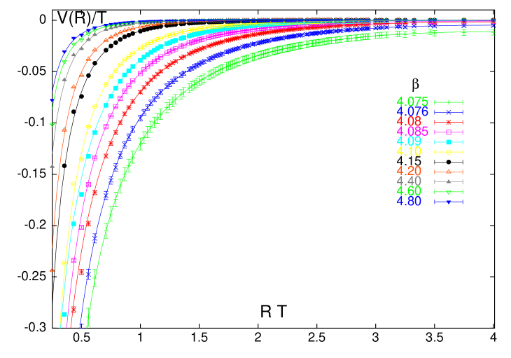
Figure 6: The potentials $V(R,T)$ for the $\beta$ values above $\beta_{c}$ analyzed on the $N_{\tau}=4$ lattices. The Polyakov loop correlations have been normalized to their cluster value. Potentials and distances are given in units of the temperature.

In the following we first concentrate on data set (I) which has somewhat better statistics and which, more important, covers the explored range of distances more densely, see Figure 6. As has been explained in section 2, we fit the potentials above $T_{c}$ with the generalized screening ansatz, eq. (13), where the exponent $d$ of the Coulomb-like part is treated as a free parameter. It turns out that the value of the exponent and the value of the screening mass $\mu$ are strongly correlated. In particular at the higher temperatures it is difficult to obtain fit results which are stable under the variation of the minimum distance included in the fit. These fluctuations have been taken into account in our estimates of the error bars.

At the highest temperatures analyzed we observed that at large quark separations the Polyakov-loop correlation decreases below the cluster value. In [18] it was argued that finite momentum contributions to the vacuum polarization tensor can give rise to a modified screening function which undershoots the exponential Debye decay at intermediate distances and approaches the infinite distance limit from below. Despite the high, yet limited precision of our data we are not in the position, however, to confirm this suggestion. Instead, we have taken an operational approach and have added an overall constant to our fit ansatz.

Figure 7: Fit results for the exponent $d$ of the Coulomb-like part of the potential above $T_{c}$, eq. (13), as a function of the temperature.

In Figure 7 we summarize the results for the exponent. At temperatures very close to $T_{c}$, the exponent $d$ is compatible with $1$. When the temperature is increased slightly, $d$ starts rising to about $1.4$ for temperatures up to $2T_{c}$. Between 2 and 3 times $T_{c}$, the exponent centers around 1.5, although the error bars tend to become rather large. A value of 2 as predicted by perturbation theory seems to be ruled out, however, in the investigated temperature range.

Figure 8: Fit results for the screening mass $\mu(T)$, eq. (13), as a function of the temperature. The lines denote the comparison with the perturbative prediction, $\mu(T)=A\ast m_{e}^{(0)}(T)$, see text.

The results for the screening mass $\mu(T)$ obtained from the same fits with eq. (13) are shown in figure 8. The screening mass turns out to be small but finite just above $T_{c}$ and rises rapidly when the temperature is increased. It reaches a value of about $2.5T$ at temperatures around $1.5T_{c}$ and seems to stabilize there also. Figure 8 also includes a comparison with lowest order perturbation theory, $\mu(T)=A\ast m_{e}^{(0)}(T)$ with $m_{e}^{(0)}(T)$ as given in eq. (11). For the temperature dependent renormalized coupling $g^{2}(T)$ the two-loop formula

$$g^{-2}(T)=2b_{0}\ln\left(\frac{2\pi T}{\Lambda_{\overline{MS}}}\right)+\frac{b_{1}}{b_{0}}\ln\left(\,2\ln\left(\frac{2\pi T}{\Lambda_{\overline{MS}}}\right)\right)$$ (18)

was used, where $T_{c}/\Lambda_{\overline{MS}}=1.14(4)$ [26, 27] and the lattice scale was set by the lowest Matsubara frequency $2\pi T$. Perturbation theory predicts the factor $A$ to be 2. Indeed, adjusting to the data points at the two highest temperatures, $T>2T_{c}$, leads to a value of $A=1.82\pm 0.15$ which is close to the prediction. However, in view of the results for the exponent $d$ we regard this as an accidental coincidence. This is further supported by analyses [12] in colour $SU(2)$ where the electric gluon mass was obtained from gluon propagators and from the singlet potential $V_{1}$, see eq (12). Here it was found that the observed mass follows a behaviour $m_{e}(T)\simeq 1.6m_{e}^{(0)}(T)$. If this result could be transferred to the case of $SU(3)$, and [10] provides some early evidence for this, we would have $\mu(T)\simeq 1\ast m_{e}(T)$ contrary to the perturbative value of 2.

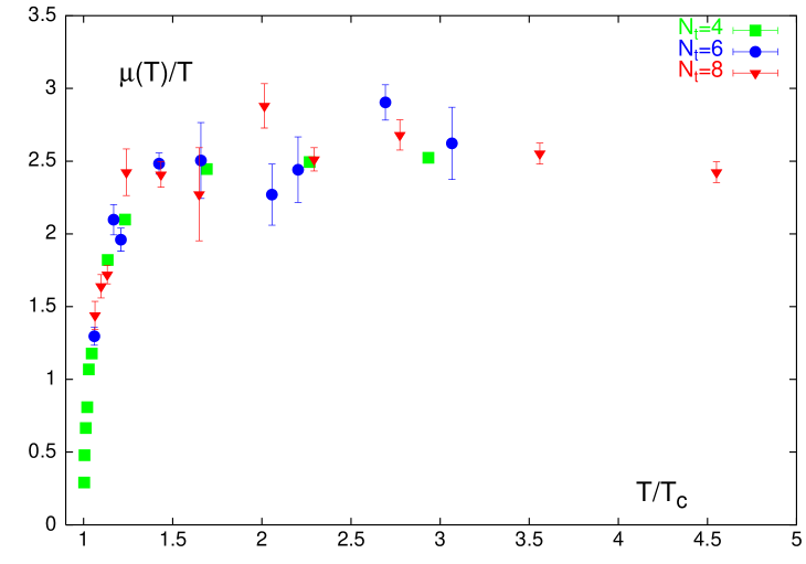
Figure 9: The screening mass $\mu$ from fits with eq. (13) with a fixed value of $d=1.5$ for the exponent. The results from all three different lattice sizes are drawn as a function of the temperature.

The potentials above $T_{c}$ from data set (II) are very similar to the ones already discussed. Fits with eq. (13) with a free exponent do work and return parameter values in the same ballpark as in case I. However, because of the much smaller number of distances probed in this set the fit results are not as reliable as in case I. Therefore we have chosen to carry out fits with eq. (13) but with $d$ kept fixed. For comparison, also data set (I) has been treated this way.

The general feature of these fits is that increasing $d$ from 1.0 to 2.0 leads to decreasing numbers for the screening mass. For instance, at $3T_{c}$ we obtain $\mu/T\approx 3$ for $d=1.0$ whereas with $d=2.0$ the result for the screening mass is $\mu/T\approx 2$. Similar shifts occur at all temperatures. The quality of the fits, however, is not always the same. Typically, at temperatures close to $T_{c}$ fits with $d=2$ return unacceptable $\raise 1.72218pt\hbox{$\chi$}^{2}$ values while for $T\geq 2T_{c}$ the $\raise 1.72218pt\hbox{$\chi$}^{2}$ values are equally good for all values of $d$ and cannot be used to distinguish between the various exponent values anymore. This observation fits nicely into the picture as shown in Figure 7.

As an example for the temperature dependence of the screening mass at fixed $d$, in Figure 9 we show our results at $d=1.5$ for all three different lattice sizes. Recall that a value of $d\approx 1.5$ was favored at all temperatures $T\raise 1.29167pt\hbox{$>$\kern-7.5pt\raise-4.73611pt\hbox{$\sim$}}1.2T_{c}$ of data set (I). The general behavior is similar to that shown in Figure 8: the screening mass is small close to $T_{c}$ and starts to rise quickly. It reaches a kind of plateau with a value of $\mu/T\approx 2.5$ for temperatures between roughly 1.5 and 3 $T_{c}$. For temperatures beyond $3T_{c}$ the $N_{\tau}=8$ data may indicate a slow decrease with rising temperature. The main conclusion to be drawn from Figure 9 is that the results from the different lattices, i.e. at different lattice spacings are in agreement with each other within the error bars. Thus, in the investigated temperature range colour screening effects are not yet properly described by simple perturbative predictions.

5 Conclusion

In this paper we have analyzed the heavy quark potential at finite temperatures in the range $0.8T_{c}$ up to about $4T_{c}$ in $SU(3)$ Yang-Mills theory. We have done so on lattices with 3 different temporal extents and found results consistent with each other. Moreover, the standard Wilson action as well as a tree-level improved Symanzik action were used. Again, consistency was observed. This indicates that finite lattice spacing artefacts are not futilizing the analysis.

The potentials at temperatures below the critical temperature of the deconfinement transition are well parametrized by formulae which have been derived within string models. In particular, the presence of a logarithmic term with the predicted strength could be established. However, the obtained string tension shows a substantial temperature dependence which is not in accord with the leading string model result. Instead, we find a decrease of the string tension which is compatible with being proportional to $(T_{c}-bT)^{1/2}$ in the critical region below $T_{c}$. At the critical temperature the string tension retains a finite value of $\sigma(T_{c})/\sigma(0)=0.121(35)$, consistent with a first order transition.

Above the deconfinement transition the potentials show a screened power-like behaviour. By comparing the data with perturbative predictions we can further strengthen earlier claims that these predictions do not properly describe the potentials up to temperatures of few times the critical one. In particular, it can be excluded that the exchange of two gluons with an effective chromo-electric mass is the dominant screening mechanism. Judging from the exponent of the $1/R$ term in the potential, at temperatures close to $T_{c}$ it seems that the complex interactions close to the phase transition arrange themselves in such a way as to be effectively describable by some kind of one-gluon exchange. At temperatures of about 1.5 to 3 times $T_{c}$ we observe a behaviour which could be interpreted as a mixture of one- and two-gluon exchange. The resulting screening mass scales with the temperature, $\mu(T)\simeq 2.5\,T$, a perturbative decrease due to the temperature-dependent renormalized coupling $g(T)$ is not really seen. Thus, it is very likely that non-perturbative phenomena and higher order perturbative contributions are needed to explain the observed screening behaviour in the investigated temperature range.

Acknowledgements:

This work was supported by the TMR network ERBFMRX-CT-970122, the DFG grant Ka 1198/4-1 and partly by the “Nederlandse Organisatie voor Wetenschappelijk Onderzoek” (NWO) via a research program of the “Stichting voor Fundamenteel Onderzoek der Materie” (FOM). The numerical work has been carried out on Quadrics QH2 and QH1 computers at the University of Bielefeld which in part have been funded by the DFG under grant Pe 340/6-1. F.K. acknowledges support through the visitor program of the Center for Computational Physics at the University of Tsukuba and thanks the CCP for the kind hospitality extended to him. E.L. thanks the NIKHEF for the kind hospitality and J. Koch for critical comments on the manuscript.

Appendix

$N_{\tau}$	$\beta$	$T/T_{c}$	$\sigma a^{2}$
4	3.95	0.804	0.2256(6)
	4.00	0.886	0.1783(4)
	4.02	0.916	0.1581(2)
	4.04	0.947	0.1339(4)
	4.05	0.963	0.1263(3)
	4.06	0.979	0.1113(8)
	4.065	0.987	0.0970(8)
	4.07	0.995	0.0882(15)
6	5.80	0.832	0.0917(10)
	5.85	0.919	0.0634(23)
	5.87	0.956	0.0526(8)
	5.89	0.993	0.0203(13)
			0.0400(20)
8	6.00	0.904	0.0386(6)
	6.04	0.967	0.0204(5)
			0.0300(15)
	6.06	0.9985	0.0078(7)
			0.0195(15)

Table 1: Results for the string tension in lattice units from fits with eq. (4). In those cases where two lines are printed for a given $\beta$ the upper line refers to averages over the whole sample while the lower line takes into account only configurations which are in the confined phase.

$N_{\tau}$	$\beta$	$T/T_{c}$	$\sigma a^{2}$
4	3.95	0.804	0.1592(8)
	4.00	0.886	0.1125(4)
	4.02	0.916	0.0925(3)
	4.04	0.947	0.0686(3)
	4.05	0.963	0.0607(3)
	4.06	0.979	0.0458(6)
	4.065	0.987	0.0316(9)
	4.07	0.995	0.0221(11)

Table 2: Results for the string tension from fits with eq. (5).

References

- [1] T. Matsui and H. Satz, Phys. Lett. B178 (1986) 416.
- [2] F. Karsch, M. T. Mehr and H. Satz, Z. Phys. C37 (1988) 617.
- [3] R. D. Pisarski and O. Alvarez, Phys. Rev. D26 (1982) 3735.
- [4] Ph. de Forcrand et al., Phys. Lett. 160B (1985) 137.
- [5] M. Gao, Phys. Rev. D40 (1989) 2708.
- [6] for a summary see A. Ukawa, Nucl. Phys. B (Proc. Suppl.) 17 (1990) 118.
- [7] J. Engels and V. Mitrjushkin, Phys. Lett. B282 (1992) 415.
- [8] T.A. DeGrand and C. DeTar, Phys. Rev. D34 (1986) 2469.
- [9] K. Kanaya and H. Satz, Phys. Rev. D34 (1986) 3193.
- [10] N. Attig et al., Phys. Lett. B209 (1988) 65.
- [11] J. Engels, F. Karsch and H. Satz, Nucl. Phys. B315 (1989) 419.
- [12] U.M. Heller, F. Karsch and J. Rank, Phys. Rev. D57 (1998) 1438.
- [13] S. Nadkarni, Phys. Rev. D33 (1986) 3738.
-
[14]
E. Manousakis and J. Polonyi, Phys. Rev. Lett. 58
(1987) 847;
J.B. Kogut and C. DeTar, Phys. Rev. D36 (1987) 2828. - [15] M. Lüscher, K. Symanzik and P. Weisz, Nucl. Phys. B173 (1980) 365.
- [16] K.J. Juge, J. Kuti and C.J. Morningstar, Nucl. Phys. Proc. Suppl. 73 (1999) 590.
- [17] A.K. Rebhan, Phys. Rev. D48 (1993) R3967; Nucl. Phys. B430 (1994) 319.
- [18] J.C. Gale and J. Kapusta, Phys. Lett. B198 (1987) 89.
- [19] G. Boyd et al., Nucl. Phys. B469 (1996) 419.
- [20] N. Cabibbo and E. Marinari, Phys. Lett. 119B (1982) 387.
-
[21]
K. Fabricius and O. Haan, Phys. Lett. 143B (1984) 459;
A. Kennedy and B. Pendleton, Phys. Lett. 156B (1985) 393. - [22] S. Adler, Phys. Rev. D23 (1981) 2901.
-
[23]
R. Brower, Nucl. Phys. B190 (1981) 699;
G. Parisi, R. Petronzio and F. Rapuano, Phys. Lett. 128B (1983) 418;
Ph. de Forcrand and C. Roiesnel, Phys. Lett. 151B (1985) 77. - [24] B. Beinlich, F. Karsch and A. Peikert, Phys. Lett. B390 (1997) 268.
- [25] R.G. Edwards, U.M. Heller and T.R. Klassen, Nucl. Phys. B517 (1998) 377.
- [26] B. Beinlich et al., Eur. Phys. J. C6 (1999) 133.
- [27] G. Bali and K. Schilling, Phys. Rev. D47 (1993) 661.