Colour confinement and dual superconductivity of the vacuum - II

Abstract

The dual superconductivity of the vacuum in $SU(3)$ gauge theory is investigated by constructing a disorder parameter which signals monopole condensation in various abelian projections and by studying numerically on the lattice its behaviour at finite temperature. We find that the vacuum is a dual superconductor with respect to each $U(1)$ of the residual gauge group after abelian projection independently of the abelian projection chosen. Like in the $SU(2)$ case (discussed in a companion paper) a finite size scaling analysis enables us to extract the indices of the phase transition and our analysis is consistent with independent determinations.

PACS numbers: 11.15.Ha, 12.38.Aw, 14.80.Hv, 64.60.Cn

I Introduction

In a companion paper [1], which we will quote as I, we have presented the basic ideas about confinement and dual superconductivity of the ground state of gauge theories, and how they can be tested in $SU(2)$ gauge theory. Monopoles exist in gauge theories, carrying a conserved magnetic charge. We have defined a disorder parameter $\langle\mu\rangle$ detecting dual superconductivity as spontaneous breaking of the $U(1)$ symmetry related to magnetic charge conservation. $\langle\mu\rangle\neq 0$ signals that the ground state is a superposition of states with different magnetic charge, a phenomenon which is denoted as condensation and which implies dual superconductivity under very general assumptions.

In $SU(2)$ a monopole species can be associated to any operator in the adjoint representation, with a corresponding magnetic $U(1)$ symmetry. Condensation can be numerically investigated for different monopole species, in connection with confinement, by lattice simulation at finite temperature. The main results of this investigation for $SU(2)$ were the following:

• monopoles defined by different abelian projections do condense in the confined phase, or $\langle\mu\rangle\neq 0$;

• at deconfinement $\langle\mu\rangle\to 0$;

• a finite size scaling analysis allows to determine the critical index $\nu$ of the correlation length, the critical $\beta$ and the index $\delta$ by which $\langle\mu\rangle\to 0$. The determination of $\nu$ agrees with the ones done by other methods, and indicates a $2$nd order phase transition. Also $\beta_{C}$ coincides within errors with the known values;

• all the monopole species considered have a similar behaviour, and show dual superconductivity.

a

Our conclusion was that confinement is an order-disorder transition. The symmetry which characterizes the dual order is not fully understood, but for sure the different $\langle\mu\rangle$’s are good disorder parameters.

In this paper we shall extend the analysis to $SU(3)$ gauge group. The essentials are not changed with respect to $SU(2)$. Some formal complications come from the coexistence of two monopole charges for each abelian projection (Sect. II). We have performed a systematic numerical investigation, for different abelian projections. Also for $SU(3)$ we find dual superconductivity in all the abelian projections that we have considered, again indicating that the guess of ref. [2] that all monopoles are physically equivalent is correct. $\langle\mu\rangle$ looks, within errors, the same for the two independent monopole charges of a given abelian projection. A finite size scaling analysis shows that the transition is first order. Numerical details and results are given in Sect. III.

Sect. IV contains some concluding remarks.

II The abelian projection. Conserved monopole charges

In analogy with the $SU(2)$ case we shall denote by

$$\phi(x)=\sum_{i=1}^{8}\phi^{i}(x)F^{i}$$ (1)

the generic local operator in the adjoint representation. $F^{i}=\lambda^{i}/2$, with $\lambda^{i}$ the Gell-Mann matrices. We shall assume $\phi$ hermitian, or $\phi^{i}$ real in any configuration.

It will be convenient to use the notation

$$\phi(x)=\vec{\phi}(x)\cdot\vec{F}$$ (2)

for eq. (1) and for any two operators $\phi_{1}$, $\phi_{2}$

$$2\mbox{tr}\phi_{1}\phi_{2}=\vec{\phi}_{1}\cdot\vec{\phi}_{2}\equiv\sum_{i=1}^{8}\phi^{i}_{1}\phi^{i}_{2}\ .$$ (3)

Any $\phi(x)$ can be diagonalized by a unitary transformation $U(x)$

$$U(x)\phi(x)U^{\dagger}(x)=\phi_{D}(x)\ .$$ (4)

In the usual representation of the $\lambda$ matrices

$$\phi_{D}=\varphi_{D}^{a}F^{a}+\varphi_{D}^{b}F^{b}\ ,$$ (5)

where $F^{a}$ and $F^{b}$ are independent linear combinations of $F^{3}$ and $F^{8}$. We shall choose

$$F^{a}=F^{8}\ ,\qquad F^{b}=\frac{\sqrt{3}}{2}F^{3}+\frac{F^{8}}{2}$$ (6)

for reasons which will be clear below.

We now define

$$f^{a}(x) = \left(U(x)\right)^{\dagger}F^{a}U(x)\ ,$$ (7)

$$f^{b}(x) = \left(U(x)\right)^{\dagger}F^{b}U(x)\ .$$ (8)

$U(x)$ is defined as the matrix which diagonalizes $\phi(x)$. To eliminate ambiguities the eigenvalues can be ordered in decreasing order. $U(x)$ is determined up to an arbitrary matrix $U_{D}(x)$ on the left $U(x)\simeq U_{D}(x)U(x)$, with $U_{D}=\exp\left(i\alpha F^{8}+i\beta F^{3}\right)$, i.e. up to a residual $U(1)^{2}$. From eq. (5) and (7), in the usual representation of Gell-Mann matrices

$$\phi_{D}=\frac{1}{2\sqrt{3}}\left(\begin{array}[]{c c c}\varphi_{D}^{a}+2\varphi_{D}^{b}&0&0\\ 0&\varphi_{D}^{a}-\varphi_{D}^{b}&0\\ 0&0&-2\varphi_{D}^{a}-\varphi_{D}^{b}\end{array}\right)\ ,$$ (12)

with $\varphi_{D}^{a}\geq 0$, $\varphi_{D}^{b}\geq 0$.

The gauge transform $U(x)$ is singular at the sites where either $\varphi_{D}^{b}=0$, and

$$\phi_{D}=\frac{1}{2\sqrt{3}}\varphi_{D}^{a}\left(\begin{array}[]{r r r}1&0&0\\ 0&1&0\\ 0&0&-2\end{array}\right)\ ,$$ (16)

or $\varphi_{D}^{a}=0$, and

$$\phi_{D}=\frac{1}{2\sqrt{3}}\varphi_{D}^{b}\left(\begin{array}[]{r r r}2&0&0\\ 0&-1&0\\ 0&0&-1\end{array}\right)\ .$$ (20)

In both cases $\phi_{D}$ has two equal eigenvalues.

The two field tensors

$$F_{\mu\nu}^{a,b}=\frac{1}{2}\mbox{tr}\left({f}^{a,b}\cdot{G}_{\mu\nu}-\frac{i}{g}{f}^{a,b}\cdot\right.$$ (21)

$$\left.\frac{4}{3}\left[D_{\mu}{f}^{a,b}\ ,\ D_{\nu}{f}^{a,b}\right]\right)$$ (22)

are the analogous of the ’t Hooft’s tensor [3] in $SU(2)$. Like in $SU(2)$ the bilinear terms in $A_{\mu}A_{\nu}$ cancel. In the abelian projected gauge $f^{a}(x)=F^{a}$ and $f^{b}(x)=F^{b}$ are $x$ independent, apart from singularities, and therefore in the domain in which $U(x)$ is regular

$$F^{a,b}_{\mu\nu}={\partial}_{\mu}A^{a,b}_{\nu}-{\partial}_{\nu}A_{\mu}^{a,b}\ .$$ (23)

The cancellation of the bilinear term $A_{\mu}A_{\nu}$ between the two terms of eq. (21) is not automatic in $SU(3)$ for arbitrary choice of $f^{a}$, $f^{b}$, as it was in $SU(2)$, and only works if $f^{a}$, $f^{b}$ belong to $U(1)$ in the breaking $SU(3)\to SU(2)\times U(1)$, which is the case for the choice of (6). Also the choice $\frac{\sqrt{3}}{2}F^{3}-\frac{1}{2}F^{8}$ for $f^{a}$ or $f^{b}$ would be legitimate.

As in $SU(2)$ $F^{a,b\star}_{\mu\nu}$, the dual tensor to $F^{a,b}_{\mu\nu}$, define two magnetic currents $\partial^{\nu}F^{a,b\star}_{\mu\nu}=j^{a,b}_{\mu}$, which are conserved. The theory has two conserved magnetic charges, $M^{a},\ M^{b}$. Monopoles exist at the points where $U(x)$ is singular: where $\varphi_{D}^{b}=0$ the monopole field is directed as $F^{3}=\mbox{diag}(\ 1/2\ ,-1/2\ ,0\ )$, where $\varphi_{D}^{a}$ is zero it is directed as $F^{3a}=-(1/2)F^{3}+(\sqrt{3}/2)F^{8}=\mbox{diag}(\ 0\ ,1/2\ ,-1/2\ )$. As in $SU(2)$ we shall investigate the invariance of the ground state with respect to these magnetic $U(1)$’s, in connection with confinement.

On the lattice, we shall define the abelian projected fields as follows. In the abelian projected representation we write the generic link $U_{\mu}(n)$ in the form

$$U_{\mu}(n)=e^{i\vec{V}_{\bot}\cdot\vec{F}_{\bot}}e^{i(V_{a}F^{a}+V_{b}F^{b})}\ ,$$ (24)

with $\vec{F}_{\bot}$ a superposition of generators belonging to non zero eigenvalues of the Cartan algebra.

Eq. (24) is easy to prove: it is a trivial consequence of the Baker-Hausdorff formula. Like for $SU(2)$, the abelian part of a product is the sum of the abelian parts of the factors, to order $a^{2}$ ($a$ is the lattice spacing). The abelian magnetic fluxes through plaquettes, one for each $U(1)$, can be defined, and are identically conserved. The disorder parameter is again

$$\langle\mu^{a,b}\rangle=\frac{Z[S+\Delta^{a,b}S]}{Z[S]}\ ,$$ (25)

$$\Delta^{a,b}S=\frac{\beta}{3}\sum_{\vec{n}}\mbox{Tr}\left\{\Pi_{i0}(\vec{n},t)-\Pi_{i0}^{\prime{a,b}}(\vec{n},t)\right\}\ ,$$ (26)

$\Pi_{i0}^{\prime{a,b}}(\vec{n},t)$ is obtained from $\Pi_{i0}(\vec{n},t)=U_{i}(\vec{n},t)U_{0}(\vec{n}+\hat{\imath},t)\left(U_{i}(\vec{n},t+1)\right)^{{\dagger}}\left(U_{0}(\vec{n},t)\right)^{{\dagger}}$ by the change

$$U_{i}(\vec{n},t) \to e^{-i\Lambda(\vec{n},\vec{y}){f}^{a,b}(\vec{n},t)}U_{i}(\vec{n},t)$$ (28)

$$e^{iA_{\bot i}^{M}(\vec{n},\vec{y}){f}^{a,b}(\vec{n}+\hat{\imath},t)}e^{i\Lambda(\vec{n}+\hat{\imath},\vec{y}){f}^{a,b}(\vec{n}+\hat{\imath},t)}\,$$

where

$$\vec{A}^{M}(\vec{n},\vec{y})=\vec{A}^{M}_{\bot}(\vec{n},\vec{y})+\vec{\nabla}\Lambda(\vec{n},\vec{y})\$$ (29)

is the vector potential produced by a monopole. The proof that $\langle\mu^{a,b}\rangle$ creates a monopoles of the corresponding type is exactly the same as for $SU(2)$.

Also for $SU(3)$ instead of $\langle\mu^{a,b}\rangle$ it is convenient to determine

$$\rho^{a,b}=\frac{\mbox{d}}{\mbox{d}\beta}\log\langle\mu^{a,b}\rangle=\langle S\rangle_{S}-\langle S+\Delta S\rangle_{S+\Delta S}$$ (30)

as a function of $\beta$. We do that on an asymmetric lattice $N_{s}^{3}\times N_{t}$ ($N_{s}\gg N_{t}$ ) which provides the static thermal equilibrium at $T=1/a(\beta)$.

The deconfining transition is known and has been studied using the Polyakov loop order parameter [4]. We will investigate if going from deconfined to confined phase monopoles do condense to produce dual superconductivity. $\langle\mu^{a,b}\rangle$ will be the disorder parameters.

III Numerical results

We determine the temperature dependence of $\rho$ on a lattice $N_{s}^{3}\times N_{t}$ ($N_{s}\gg N_{t}$), with $N_{t}=4$ and $N_{s}$ ranging from 12 to 32. For the reason discussed in [1], we use periodic boundary conditions in the spatial directions and $C^{\star}$-boundary conditions [5] in the time direction. As in $SU(2)$ we diagonalize an operator ${\cal O}$ belonging to the group ${\cal O}=\exp(i\Phi^{a}\lambda^{a}/2)$ and we identify $\Phi^{a}$ by ordering the imaginary part of eigenvalues in decreasing order.

As for the $SU(2)$ case, we study the following projections:

• ${\cal O}$ is connected to the Polyakov line $L(\vec{n},t)=\Pi_{t^{\prime}=t}^{N_{t}-1}U_{0}(\vec{n},t^{\prime})\Pi_{t^{\prime}=0}^{t-1}U_{0}(\vec{n},t^{\prime})$ in the following way:

  $${\cal O}(\vec{n},t)=\Pi_{t^{\prime}=t}^{N_{t}-1}U_{0}(\vec{n},t^{\prime})L^{\star}(\vec{n},0)\Pi_{t^{\prime}=0}^{t-1}U_{0}(\vec{n},t^{\prime})\ ;$$ (31)

  (Polyakov projection on a $C^{\star}$-periodic lattice);

• ${\cal O}$ is an open plaquette, i.e. a parallel transport on an elementary square of the lattice

  $${\cal O}(n) = \Pi_{ij}(n)$$ (32)

  $$= U_{i}(n)U_{j}(n+\hat{\imath})\left(U_{i}(n+\hat{\jmath})\right)^{{\dagger}}\left(U_{j}(n)\right)^{{\dagger}}\ ;$$ (33)

• ${\cal O}$ is the “butterfly” $F$

  $${\cal O}(n) = F(n)$$ (34)

  $$= U_{x}(n)U_{y}(n+\hat{x})\left(U_{x}(n+\hat{y})\right)^{{\dagger}}\left(U_{y}(n)\right)^{{\dagger}}$$ (36)

  $$U_{z}(n)U_{t}(n+\hat{z})\left(U_{z}(n+\hat{t})\right)^{{\dagger}}\left(U_{t}(n)\right)^{{\dagger}}\ .$$

The trace of $F$ is the density of topological charge.

The simulation was done on a 128-node APE Quadrics Machine. We use an overrelaxed heat-bath algorithm to compute the Wilson term of eq. (30), and a mixed algorithm as described in our previous paper [1] for the monopole term $\langle S+\Delta S\rangle_{S+\Delta S}$. Far from the critical region at each $\beta$ we sampled over 4000 termalized configurations, each of them taken after 4 sweeps. The errors have been obtained by using a Jackknife method on binned data, as discussed in [1]. In the critical region a higher statistics is required. Typically the Wilson term is more noisy. Thermalization was checked by monitoring the action density and the probability distribution of the trace of the Polyakov loop. The number of measurements was at least $300\tau_{C}$, where $\tau_{C}$ is the correlation time of the considered set of data.

For $\vec{A}_{\bot}$ we use the Wu-Yang’s parameterization; we have also checked numerically that Dirac’s form gives similar results, as expected.

In terms of $\rho$

$$\langle\mu^{a,b}\rangle=\exp\left(\int_{0}^{\beta}\rho^{a,b}(\beta^{\prime})\mbox{d}\beta^{\prime}\right)\ .$$ (37)

Eq. (37) implies that if the dual $U(1)$ symmetry defined by some abelian projection and by some abelian generator of the gauge group is related to colour confinement, in the thermodynamic limit $N_{s}\to\infty$ the corresponding $\rho$ stays finite in the strong coupling region ($\beta<\beta_{C}$) and goes to $-\infty$ linearly with $N_{s}$ in the weak coupling region ($\beta>\beta_{C}$). In the critical region, the abrupt decline of $\langle\mu\rangle$ is signaled by a sharp negative peak of $\rho$; the value of $\rho$ in this region must behave as a function of $N_{s}$ as prescribed by the finite size scaling theory of pseudocritical systems.

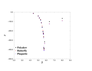
FIG. 1.: $\rho$ vs. $\beta$ for different abelian projections. Lattice $12^{3}\times 4$, abelian generator $F^{3}$.

Fig. 1 shows the typical behaviour of $\rho$ for different abelian projections, for a lattice $12^{3}\times 4$. As abelian generator we used $F^{3}$. The negative peak occurs at the expected transition point, $\beta_{C}$ [6]. Below $\beta_{C}$ the different projections are equal within errors, suggesting that different monopoles behave in the same way.

We have investigated also whether at fixed abelian projection the profile of $\rho$ depends on the $U(1)$ magnetic subgroup. Fig 2 shows the profile of $\rho$ corresponding to $F^{3},F^{8}$ and $F^{3a}$ in the Polyakov projection on a $12^{3}\times 4$ lattice. No appreciable differences can be seen between different choices. This is an indication (confirmed also by simulations on larger lattices) that monopoles defined with respect to different abelian generators behave in the same way in the $SU(3)$ vacuum. This is also true for the other abelian projections we have investigated (see fig. 1).

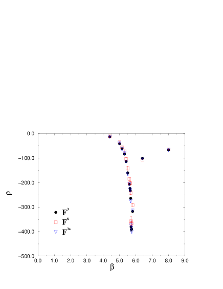
FIG. 2.: $\rho$ vs. $\beta$ for different abelian generators. Lattice $12^{3}\times 4$, Polyakov projection.

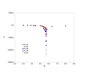
FIG. 3.: $\rho$ as a function of $\beta$ for different spatial sizes at fixed $N_{t}=4$. Polyakov projection, abelian generator $F^{3}$.

Since different abelian projections and different abelian generators give indistinguishable results, for the sake of simplicity we shall only display the Polyakov projection and the abelian generator $F^{3}$ in the following figures.

Fig. 3 shows the dependence of $\rho$ on $N_{s}$. The qualitative behaviour does not change when we enlarge the lattice size.

We now analyze the dependence on $N_{s}$ in more detail.

In the strong coupling region at low $\beta$’s $\rho$ seems to converge to a finite value (cfr. fig. 4). Eq. (37) then implies that $\langle\mu\rangle\neq 0$ in the infinite volume limit in the confined phase for these $\beta$’s. Hence monopoles do condense in this phase.

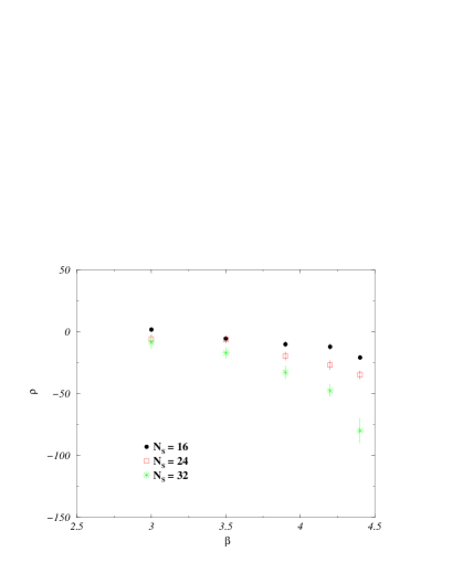
FIG. 4.: $\rho$ vs. $\beta$ in the strong coupling region for lattice sizes $N_{s}^{3}\times 4$. Polyakov projection, abelian generator $F^{3}$.

FIG. 5.: $\rho$ vs. $N_{s}$ ($N_{t}=4$) at $\beta=\infty$ in the Polyakov projection with abelian generator $F^{3}$. Data are obtained by numerical minimization of $\langle S+\Delta S\rangle_{S+\Delta S}$.

In the weak coupling region, we can evaluate $\rho$ perturbatively. The path integral is then dominated by the classical solutions of the equations of motion for the gauge variables and we have

$$\rho \mathop{\to}_{\beta\to\infty}\left[\mathop{\min}_{U}\{S\}-\mathop{\min}_{U}\{S+\Delta S\}\right]$$ (39)

$$\ =-\mathop{\min}_{U}\{S+\Delta S\}\ ,$$

since $\mathop{\min}_{U}\{S\}=0$.

In other systems, where the same shifting procedure has been applied and studied, this asymptotic value has been analytically calculated in perturbation theory with the result [7, 8]

$$\rho=-cN_{s}+d\ ,$$ (40)

where $c$ and $d$ are constants, i.e $\rho$ goes linearly with the spatial dimension.

In $SU(3)$ we are unable to perform the same calculation and we have evaluated the minimum $\mathop{\min}_{U}\{S+\Delta S\}$ numerically. Detail about the followed procedure have been discussed in [1]. Here we note that due to the single precision of the APE Quadrics Machine, the estimation of the minimum of $S+\Delta S$ for the biggest lattice is more noisy than in the $SU(2)$ case.

The result is shown in fig. 5 for the Polyakov projection. It is consistent with the linear dependence of eq. (40) with $c\simeq 2$ and $d\simeq-12$. Thus in the weak coupling region in the thermodynamic limit $\rho$ goes to $-\infty$ linearly with the spatial lattice size and

$$\langle\mu\rangle\mathop{\approx}_{N_{s}\to\infty}Ae^{(-cN_{s}+d)\beta}\to 0,\quad\beta>\beta_{C}\ .$$ (41)

The magnetic $U(1)$ symmetry is indeed restored in the deconfined phase.

The behaviour of $\rho$ in the critical region can be investigated by using finite size scaling techniques. We know that the transition is weak first order with a behaviour which is difficult to distinguish from that of a second order transition.

By dimensional argument

$$\langle\mu\rangle=N_{s}^{-\delta/\nu}\Phi\left(\frac{\xi}{N_{s}},\frac{a}{\xi},\frac{N_{t}}{N_{s}}\right)\ ,$$ (42)

where $a$ and $\xi$ are respectively the lattice spacing and the correlation length of the system.

Near the critical point, for $\beta<\beta_{C}$

$$\xi\propto\left(\beta_{C}-\beta\right)^{-\nu},$$ (43)

where $\nu$ is some effective critical exponent. In the limit $N_{s}\gg N_{t}$ and for $a/\xi\ll 1$, i.e. sufficiently close to the critical point we obtain

$$\langle\mu\rangle=N_{s}^{-\delta/\nu}\Phi\left(N_{s}^{1/\nu}\left(\beta_{C}-\beta\right),0,0\right)$$ (44)

or equivalently

$$\frac{\rho}{N_{s}^{1/\nu}}=f\left(N_{s}^{1/\nu}\left(\beta_{C}-\beta\right)\right)\ .$$ (45)

The ratio $\rho/N_{s}^{1/\nu}$ is a universal function of the scaling variable

$$x=N_{s}^{1/\nu}\left(\beta_{C}-\beta\right)\ .$$ (46)

For a pseudocritical behaviour, we expect $\nu=1/3$. Using also $\beta_{C}(N_{t}=4)=5.6925$ [6], we can plot $\rho/N_{s}^{1/\nu}$ as a function of $x$.

If we perform such a plot, we find that the scaling relation (45) does not hold. Such a scaling violation is due to finite size effect. A relationship more appropriate than (45) is

$$\frac{\rho}{N_{s}^{1/\nu}}=f\left(N_{s}^{1/\nu}\left(\beta_{C}-\beta\right)\right)+\Phi(N_{s})\ ,$$ (47)

where $\Phi(N_{s})$ parameterizes finite size effects. If we assume that these effects are not critical [9] then $\Phi$ is given by

$$\Phi(N_{s})=\frac{a}{N_{s}^{3}}\ ,$$ (48)

where $a$ is a constant. This parameterization is correct ${\cal O}(1/N_{s}^{6})$.

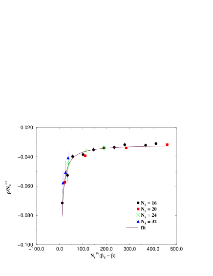
FIG. 6.: Quality of scaling in the Polyakov projection at $N_{t}=4$. Abelian generator $F^{3}$.

Fig. 6 shows the quality of the scaling for $a=190$. Our estimate gives $\nu=0.33\pm 0.07$ and $a=190\pm 20$.

In the thermodynamic limit in some region of $\beta<\beta_{C}$ we expect

$$\langle\mu\rangle\propto\left(\beta_{C}-\beta\right)^{\delta}\ ,$$ (49)

which implies

$$\frac{\rho}{N_{s}^{1/\nu}}=-\frac{\delta}{x}\ .$$ (50)

Using eq. (50) it should be possible in principle to determine $\nu$, $\delta$ and $\beta_{C}$. Our statistic is not enough accurate to perform such a fit. However, we can determine $\delta$ using as an input $\beta_{C}$, $\nu$, which are known, by parameterizing $\rho$ in a wide range by the form

$$\frac{\rho}{N_{s}^{1/\nu}}=-\frac{\delta}{x}-c+\frac{a}{N_{s}^{3}}\ ,$$ (51)

where $c$ is a constant, as suggested by fig. 6.

Our best fit $\delta=0.54\pm 0.04$ for the Polyakov projection and compatible results for the other projections. The $\chi^{2}$ is order 1.

This concludes our argument about the thermodynamic limit ($N_{s}\to\infty$). The deconfining phase transition can be seen from a dual point of view as the transition of the vacuum from the dual superconductivity phase to the dual ordinary phase. That feature seems to be independent of the abelian projection and of the abelian generator chosen.

IV Concluding remarks

Like for $SU(2)$, also for $SU(3)$ gauge theory we have found evidence that transition to deconfinement is an order-disorder transition, the disorder parameter being a condensate of magnetic charges. A finite size scaling analysis of the system gives critical indices compatible with a first order transition, in agreement with determinations done by other methods [4].

Of course we have investigated a limited number of abelian projections: like in $SU(2)$, however, the indication is that physics is independent of that choice.

An interesting issue would be to investigate if the mechanism is the same in the $N_{c}=\infty$ limit. As a consequence also in the presence of dynamical quarks the behaviour should be similar, as well as the symmetry pattern and the disorder parameter should be the same. Investigation in this direction is on the way.

REFERENCES

- [1] A. Di Giacomo, B. Lucini, L. Montesi, G. Paffuti, Colour confinement and dual superconductivity of the vacuum - I, preprint IFUP-TH 35/99, available as hep-lat/9906024.
- [2] G. ’t Hooft, Nucl. Phys. B190, 455 (1981).
- [3] G. ’t Hooft, Nucl. Phys. B79, 276 (1974).
- [4] M. Fukugita, M. Okawa, A. Ukawa, Phys. Rev. Lett. 63, 1768 (1989).
- [5] U.J. Wiese, Nucl. Phys. B375, 45 (1992).
- [6] G. Boyd, J. Engels, F. Karsch, E. Laermann, C. Legeland, M. Lütgemeier, B. Petersson, Phys. Rev. Lett. 75, 4169 (1995).
- [7] G. Di Cecio, A. Di Giacomo, G. Paffuti, M. Trigiante, Nucl. Phys. B489, 739 (1997).
- [8] A. Di Giacomo, G. Paffuti, Phys. Rev. D56, 6816 (1997).
- [9] N.A. Alves, B.A. Berg, S. Sanielevici, Nucl. Phys. B376, 218 (1992).