Colour confinement and dual superconductivity of the vacuum - I

Abstract

We study dual superconductivity of the ground state of $SU(2)$ gauge theory, in connection with confinement. We do that measuring on the lattice a disorder parameter describing condensation of monopoles. Confinement appears as a transition to dual superconductor, independent of the abelian projection defining monopoles. Some speculations are made on the existence of a more appropriate disorder parameter. A similar study for $SU(3)$ is presented in a companion paper.

PACS numbers: 11.15.Ha, 12.38.Aw, 14.80.Hv, 64.60.Cn

I Introduction

Order-disorder duality [1, 2] plays an increasingly important rôle in our understanding of the dynamics of gauge theories, specifically of QCD [3, 4] and of its supersymmetric generalizations [5].

Duality is typical of systems which can have configurations with non trivial spatial topology, carrying a conserved topological charge. The prototype example is the $2d$ Ising model. If viewed as a discretized version of a $1+1$ dimensional field theory, it presents one-dimensional configurations, kinks, whose topology is determined by the boundary conditions ($\pm 1$) at $x_{1}=\pm\infty$.

In the usual description in terms of the local variable $\sigma(x)=\pm 1$, at low temperature (weak coupling) the system is in an ordered phase with nonzero magnetization $\langle\sigma\rangle\neq 0$. At the critical point $\langle\sigma\rangle\to 0$ and the system becomes disordered. $\langle\sigma\rangle$ is called an order parameter. However one can describe the system in terms of a dual variable $\sigma^{\star}$, on a dual lattice. A dual $1d$ configuration with one $\sigma^{\star}$ up is a kink, which is a highly non local object in terms of $\sigma$. In ref. [2] it was shown that the partition function in terms of $\sigma^{\star}$ has the same form as in terms of $\sigma$, i.e. that the system with dual description looks again as an Ising model, except that the new Boltzmann factor $\beta^{\star}$ is related to the old one $\beta$ by the relation

$$\sinh\left(2\beta^{\star}\right)=\frac{1}{\sinh\left(2\beta\right)}\ .$$ (1)

The disordered phase is an ordered phase for the dual and viceversa. In the disordered phase $\langle\sigma^{\star}\rangle\neq 0$: kinks condense in the ground state. $\langle\sigma^{\star}\rangle$ is called a disorder parameter. $\sigma^{\star}$ is a dual variable to $\sigma$. In this specific case the system is self dual, and duality transformation maps the strong coupling regime in the weak coupling regime and viceversa.

a

Other systems showing duality properties are the $3d$ $XY$ model, whose dual is a Coulomb gas in $3d$, and the compact $U(1)$ gauge theory.

In the $3d$ $XY$ model topological excitations are the vortices of the $2d$ $XY$ model. These vortices condense in the disordered phase [6].

For $U(1)$ theory topological excitations are monopoles. There the duality transformation can be performed for special choices of the action (e.g. the Villain action [7], dual to a $\mathbb{Z}$ gauge theory, and the Wilson action [8]). For other choices it is not known how to explicitly perform the transformation to the dual.

An alternative approach consists in identifying the symmetry which is spontaneously broken in the disordered phase, i.e. the topological configurations which are supposed to condense, and in writing a disorder parameter in terms of the original local fields [9]. The disorder parameter is then the vacuum expectation value (vev) of a non local operator.

This approach has been translated on the lattice [10, 11], tested by numerical simulations in the compact $U(1)$ gauge theory [12], in the $3d$ $XY$ model [6] and in the $O(3)$ sigma model [13], and first used to investigate colour confinement in QCD in ref. [14].

In the early literature on the subject condensation was demonstrated as the sudden increase of the density of topological excitations. This is incorrect, since disorder can only be described by the vev of an operator which violates the dual symmetry and the number of excitations does not.

Looking at symmetry is specially important in QCD. For QCD there exists some general idea about the dual [3, 15]. The dual description should also be a gauge theory, possibly with interchange of the rôle of electric and magnetic quantities.

This idea could fit the mechanism for confinement of colour proposed in ref.’s [16, 17] as dual superconductivity of the ground state, if confinement were due to disorder and monopoles were the topological excitations which condense. However a dual superconductor is a typically abelian system, while the disorder parameter is expected to break a non abelian symmetry. An abelian conserved monopole charge can be associated to each operator in the adjoint representation by a procedure which is known as abelian projection [18]. We will recall that procedure in Sect. II. There exists a functional infinity of choices for the operator, and correspondingly an infinity of monopole species. A possibility is that the true disorder symmetry implies the condensation of all these species of monopoles [18]. Some people believe instead that some abelian projection (specifically the Maximal Abelian one) identifies monopoles that are more relevant than others for confinement. Both attitudes reflect our ignorance of the dual description of the system.

In this paper we shall systematically explore condensation of monopoles defined by different abelian projections, in connection with confinement of colour.

We will do that for $SU(2)$ gauge theory. The treatment of $SU(3)$ will be given in a companion paper. Some of the results have been obtained during the last years and have been reported to conferences and workshops [10, 19, 20]. This paper contains conclusive results, and is an organic report of the methods and of the results obtained after ref. [14].

Our strategy consists in constructing an operator with non zero magnetic charge, for each abelian projection (Sect. III). Its vev is a candidate disorder parameter for dual superconductivity of the ground state. We shall determine numerically that vev at finite temperature below and above the deconfining phase transition. If condensation of these monopoles is related to confinement, we expect the disorder parameter to be zero in the deconfined phase, and different from zero in the confined phase.

This is strictly speaking true only in the thermodynamic (infinite volume) limit. A finite size scaling analysis allows to go to that limit, and, as a by-product, gives a determination of the transition temperature and of the critical indices if the transition is higher order than first. This analysis is presented in Sect. IV.

A special treatment for the Maximal Abelian projection is presented in Sect. V.

We find that gauge theory vacuum is indeed a dual superconductor in the confined phase, and becomes normal in the deconfined phase for a number of abelian projections, actually for all projections that we have analyzed, in agreement with the guess of ref. [18].

The idea that confinement is produced by dual superconductivity is thus definitely confirmed. The guess that all the abelian projections are physically equivalent is also supported, and this is an important piece of information on the way to understand the true dual symmetry.

We find evidence that $SU(2)$ deconfining transition is second order. In next paper we will show that for $SU(3)$ this transition is first order.

An analysis of full QCD, including quarks, is on the way; if the mechanism proved to be the same, the idea that quarks are a kind of perturbation, and that the dynamics is determined by gluons would be tested. This would also be a test of the ansatz that the theory already contains its essential dynamics at $N_{c}=\infty$, and that the presence of fermions and the extrapolation to $N_{c}=3$ can be viewed as perturbations.

The results are summarized in Sect. VI.

II The abelian projection

What follows will refer to the case of gauge group $SU(2)$. Adaptation to $SU(3)$ will be described in the companion paper.

Let $\hat{\Phi}(x)$ be the direction in colour space of any local operator $\vec{\Phi}(x)$, belonging to the adjoint representation of $SU(2)$. A gauge transformation $g(x)$ which rotates $\hat{\Phi}(x)$ to $(0,0,1)$, or which diagonalizes $\hat{\Phi}(x)\cdot\vec{\sigma}$ is called the abelian projection on $\vec{\Phi}(x)$. $g(x)$ can be singular in a configuration at the points where $\vec{\Phi}(x)$ has zeros, and $\hat{\Phi}(x)$ is not defined.

The field strength $F_{\mu\nu}$, defined as [21]

$$F_{\mu\nu}=\hat{\Phi}(x)\cdot\vec{G}_{\mu\nu}-\frac{1}{g}\left(D_{\mu}\hat{\Phi}(x)\wedge D_{\nu}\hat{\Phi}(x)\right)\cdot\hat{\Phi}(x)$$ (2)

is a colour singlet, and is invariant under non singular gauge transformations.

In general eq. (2) can be written as [22]

$$F_{\mu\nu} = {\partial}_{\mu}\tilde{A}_{\nu}-{\partial}_{\nu}\tilde{A}_{\mu}$$ (3)

$$- \frac{1}{g}\left(\partial_{\mu}\hat{\Phi}(x)\wedge\partial_{\nu}\hat{\Phi}(x)\right)\cdot\hat{\Phi}(x)\ .$$ (4)

with

$$\tilde{A}_{\mu}=\hat{\Phi}^{a}A_{\mu}^{a}\ .$$ (5)

In the abelian projected gauge $\hat{\Phi}(x)$ is constant, the second term in the right hand side of eq. (3) vanishes and the field $F_{\mu\nu}$ becomes an abelian field.

Denoting by $F^{\star}_{\mu\nu}$ the usual dual tensor,

$$F^{\star}_{\mu\nu}=\frac{1}{2}\epsilon_{\mu\nu\rho\sigma}F^{\rho\sigma}\ ,$$ (6)

and defining the magnetic current as

$$j_{\mu} = {\partial}^{\nu}{F}^{\star}_{\mu\nu}\ ,$$ (7)

it follows from eq.’s (3), (6), (7) that

$$\partial^{\mu}j_{\mu}=0\ .$$ (8)

The magnetic charge is conserved, and defines a magnetic $U(1)$ symmetry.

The abelian projection $g(x)$ can have singularities and as a consequence an additional field strength adds to the usual covariant gauge transform of $G_{\mu\nu}$ [21].

After abelian projection

$$G_{\mu\nu}=gG_{\mu\nu}g^{-1}+G_{\mu\nu}^{sing}\ ,$$ (9)

with $\vec{G}_{\mu\nu}^{sing}=\hat{\Phi}(x)\left(\partial_{\mu}\tilde{A}_{\nu}^{sing}-\partial_{\nu}\tilde{A}_{\mu}^{sing}\right)$ parallel to the colour direction $\hat{\Phi}(x)$, and consisting of Dirac strings starting at the zeros of $\vec{\Phi}(x)$. The field configurations contain monopoles at the zeros of $\vec{\Phi}(x)$, as sinks or sources of the regular field, and the strings carry away the corresponding magnetic flux.

On a lattice (or in any other compact regularized description in terms of parallel transport) the Dirac string reduces to an additional flux of $2\pi$ across a sequence of plaquettes, which is invisible [23].

The mechanism relating confinement of colour to dual superconductivity of the vacuum advocates a spontaneous breaking à la Higgs of the magnetic $U(1)$ symmetry described by (8), which constrains the electric component of the field eq. (3) into flux tubes.

All particles which have non zero electric charge with respect to the residual $U(1)$ (3) will then be confined. There exist coloured states, e.g. the gluon oriented parallel to $\hat{\Phi}(x)$ which are not confined. This is a strong argument that, if dual superconductivity is a mechanism of confinement at all, it must exist in many different abelian projections, as a manifestation of non abelian disorder.

On the lattice the abelian gauge field corresponding to any given projection, or $\hat{\Phi}(x)$, is extracted as follows [24].

Let $\bar{U}_{\mu}(n)=g(n)U_{\mu}(n)g^{\dagger}(n)$ be the generic link after abelian projection. We adopt the usual notation $U_{\mu}(n)\equiv U_{\mu}(\vec{n},t)\equiv\exp(iA_{\mu}(n))$, with $A_{\mu}(n)=\vec{A}_{\mu}(n)\cdot\vec{\sigma}$.

The representation in terms of Euler angles has the form

$$\bar{U}_{\mu} = e^{i\alpha_{\mu}\sigma_{3}}e^{i\gamma_{\mu}\sigma_{2}}e^{i\beta_{\mu}\sigma_{3}}$$ (10)

$$= e^{i\alpha_{\mu}\sigma_{3}}e^{i\gamma_{\mu}\sigma_{2}}e^{-i\alpha_{\mu}\sigma_{3}}e^{i\left(\beta_{\mu}+\alpha_{\mu}\right)\sigma_{3}}$$ (11)

$$= e^{i\vec{\gamma}_{\mu}^{T}\cdot\vec{\sigma}}e^{i\theta_{\mu}\sigma_{3}}\ ,\qquad\theta_{\mu}=\alpha_{\mu}+\beta_{\mu}\ ,$$ (12)

and $\vec{\gamma}^{T}$ is a vector perpendicular to the $3$ axis. We assume the usual representation in which $\sigma_{3}$ is diagonal.

For a plaquette, a similar decomposition can be performed,

$$\Pi_{\mu\nu}=e^{i\vec{\gamma}^{T}_{\mu\nu}\cdot\vec{\sigma}}e^{i\theta_{\mu\nu}\sigma_{3}}\ ,$$ (13)

$\theta_{\mu\nu}=\triangle_{\mu}\theta_{\nu}-\triangle_{\nu}\theta_{\mu}$ up to terms ${\cal O}(a^{2})$. $\theta_{\mu\nu}$ is the lattice analog of $F_{\mu\nu}$. The abelian magnetic flux is conserved by construction. A monopole appears whenever the flux entering five faces of a spatial cube adds to more than $2\pi$: then the flux through the sixth face is larger than $2\pi$, but multiples of $2\pi$ are invisible in the exponent. Formally [23]

$$\theta_{\mu\nu}=\bar{\theta}_{\mu\nu}+2\pi n_{\mu\nu}\ ,$$ (14)

with $-\pi<\bar{\theta}_{\mu\nu}<\pi$. A string through the sixth face takes care of the flux which has disappeared.

We shall construct a disorder parameter for monopole condensation as the vev of an operator carrying non zero magnetic charge, $\mu$. $\langle\mu\rangle\neq 0$ will signal dual superconductivity.

III The disorder parameter

The disorder parameter will be constructed on the same lines as in ref.’s [6, 12].

An improvement exists with respect to ref. [14], which consists in properly taking the compactness into account: in ref. [14] the approximation was that the field was treated as non compact. The same improvement was done in ref. [12] with respect to ref. [11].

All the results presented in ref.’s [20] already contain such improvement.

We first analyze the case in which $\vec{\Phi}(x)$ is determined by the Wilson Polyakov line, i.e. the closed parallel transport to $+\infty$ along the time axis and back from $-\infty$ to the initial point via the periodic boundary conditions. For this choice, after abelian projection all the links $U_{0}(n)$ along the temporal axis are diagonal, of the form $\bar{U}_{0}(n)\equiv\exp(iA^{3}_{0}(n)\sigma_{3})$.

Assuming for sake of definiteness the Wilson action we construct the operator $\mu(\vec{y},t)$ which creates a monopole at site $\vec{y}$ and time $t$ with the following recipe (a similar construction can be made for other action).

Let $\vec{A}^{M}(\vec{x},\vec{y})$ be the vector potential describing the field value at site $\vec{x}$ of a static monopole sitting at $\vec{y}$. We shall write it as

$$\vec{A}^{M}(\vec{x},\vec{y})=\vec{A}^{M}_{\bot}(\vec{x},\vec{y})+\vec{\nabla}\Lambda(\vec{x},\vec{y})\ ,$$ (15)

with $\vec{\nabla}\cdot\vec{A}^{M}_{\bot}(\vec{x},\vec{y})=0$.

The first term describes the physical part of $\vec{A}^{M}$, the second term the classical gauge freedom.

Let $\Pi_{i0}$ be the electric field plaquette at time $t$. Then we define

$$\mu=\exp\left[-\beta\Delta S\right]\ ,$$ (16)

$$\Delta S=\frac{1}{2}\sum_{\vec{n}}\mbox{Tr}\left\{\Pi_{i0}(\vec{n},t)-\Pi_{i0}^{\prime}(\vec{n},t)\right\}\ .$$ (17)

Here

$$\Pi_{i0}(\vec{n},t) = U_{i}(\vec{n},t)U_{0}(\vec{n}+\hat{\imath},t)$$ (19)

$$\left(U_{i}(\vec{n},t+1)\right)^{{\dagger}}\left(U_{0}(\vec{n},t)\right)^{{\dagger}}$$

is the electric field term of the action, and $\Pi^{\prime}_{i0}$ is a modification of it, defined as

$$\Pi_{i0}(\vec{n},t)^{\prime} = U_{i}(\vec{n},t)U_{0}(\vec{n}+\hat{\imath},t)$$ (21)

$$\left(U_{i}^{\prime}(\vec{n},t+1)\right)^{{\dagger}}\left(U_{0}(\vec{n},t)\right)^{{\dagger}}\ ,$$

$$U_{i}^{\prime}(\vec{n},t+1) = e^{i\Lambda(\vec{n},\vec{y})\hat{\Phi}(\vec{n},t)\cdot\vec{\sigma}}U_{i}(\vec{n},t)$$ (23)

$$e^{-iA_{\bot i}^{M}(\vec{n},\vec{y})\hat{\Phi}(\vec{n}+\hat{\imath},t)\cdot\vec{\sigma}}e^{-i\Lambda(\vec{n}+\hat{\imath},\vec{y})\hat{\Phi}(\vec{n}+\hat{\imath},t)\cdot\vec{\sigma}}\ .$$

The disorder parameter is defined as $\langle\mu\rangle$, or

$$\langle\mu\rangle=\frac{\int\left({\cal D}U\right)e^{-\beta(S+\Delta S)}}{\int\left({\cal D}U\right)e^{-\beta S}}\ .$$ (24)

It follows from the definition (17) that adding $\Delta S$ to the action amounts to replace the term $\Pi_{i0}$ at time $t$ with $\Pi_{i0}^{\prime}$.

The $\Pi_{i0}(\vec{n},t)$ are the only terms in the action where the $U_{0}(\vec{n},t)$ appear. In the path integral (24) a change of variables $U_{0}(\vec{n},t)\to U^{\prime}_{0}(\vec{n},t)=U_{0}(\vec{n},t)e^{i\Lambda(\vec{n},\vec{y})\hat{\Phi}(\vec{n},t)\cdot\vec{\sigma}}$ leaves the Haar measure invariant and reabsorbs the unphysical gauge factor of eq. (23), so that $\langle\mu\rangle$ is independent, as it must be, of the choice of the classical gauge for the field produced by the monopole.

Also a change of variables can be made

$$U_{i}(\vec{n},t+1)\to U_{i}(\vec{n},t+1)e^{iA_{\bot i}^{M}(\vec{n},\vec{y})\hat{\Phi}(\vec{n}+\hat{\imath},t)\cdot\vec{\sigma}}\ .$$ (25)

Again, this leaves the measure invariant, and brings $\Pi_{i0}(\vec{n},t)$ to its original form. However in the plaquette $\Pi_{ij}(\vec{n},t+1)$ it produces the change $U_{i}(\vec{n},t+1)\to U_{i}(\vec{n},t+1)e^{iA_{\bot i}^{M}(\vec{n},\vec{y})\hat{\Phi}(\vec{n}+\hat{\imath},t)\cdot\vec{\sigma}}$. By the construction of Sect. II this amounts to change, in the abelian projected gauge

$$\theta_{ij}(\vec{n},t+1) \to \theta_{ij}(\vec{n},t+1)+$$ (27)

$$\triangle_{i}A_{\bot j}^{M}(\vec{n},\vec{y})-\triangle_{j}A_{\bot i}^{M}(\vec{n},\vec{y})$$

or to add the magnetic field of a monopole.

The same redefinition of variables reflects in the change

$$\Pi_{i0}(\vec{n},t+1)\to\Pi^{\prime}_{i0}(\vec{n},t+1)\ ,$$ (28)

analogous to equation (21). Again the gauge factors $e^{-i\Lambda(\vec{n},\vec{y})\hat{\Phi}(\vec{n},t)\cdot\vec{\sigma}}$, $e^{i\Lambda(\vec{n}+\hat{\imath},\vec{y})\hat{\Phi}(\vec{n}+\hat{\imath},t)\cdot\vec{\sigma}}$ are irrelevant, since they can be reabsorbed in a redefinition of $U_{0}(\vec{n},t+1)$ . $e^{iA_{\bot i}^{M}(\vec{n},\vec{y})\hat{\Phi}(\vec{n}+\hat{\imath},t)\cdot\vec{\sigma}}$ commutes with $U_{0}(\vec{n}+\hat{\imath},t+1)$, which is diagonal with it by definition of the Polyakov line abelian projection.

In detail

$$\Pi_{i0}^{\prime}(\vec{n},t+1) = U_{i}(\vec{n},t+1)e^{iA_{\bot i}^{M}(\vec{n},\vec{y})\hat{\Phi}(\vec{n}+\hat{\imath},t)\cdot\vec{\sigma}}$$ (31)

$$U_{0}(\vec{n}+\hat{\imath},t+1)$$

$$\left(U_{i}(\vec{n},t+2)\right)^{{\dagger}}\left(U_{0}(\vec{n},t+1)\right)^{{\dagger}}$$

$$= U_{i}(\vec{n},t+1)U_{0}(\vec{n}+\hat{\imath},t+1)$$ (33)

$$e^{iA_{\bot i}^{M}(\vec{n},\vec{y})\hat{\Phi}(\vec{n}+\hat{\imath},t)\cdot\vec{\sigma}}$$

$$\left(U_{i}(\vec{n},t+2)\right)^{{\dagger}}\left(U_{0}(\vec{n},t+1)\right)^{{\dagger}}\ .$$ (34)

A new change of variable can be done analogous to (25), exposing now a monopole at $t+2$ and producing a change $\Pi_{i0}(\vec{n},t+2)\to\Pi^{\prime}_{i0}(\vec{n},t+2)$. The procedure can be iterated. If an antimonopole is created at $t+T$, by an operator analogous to that of (16), but with $\vec{A}_{\bot}^{M}\to-\vec{A}_{\bot}^{M}$, then at time $t+T$ the change cancels and the procedure stops.

This shows that the correlation function

$${\cal D}(T)=\langle\bar{\mu}(\vec{y},t+T)\mu(\vec{y},t)\rangle$$ (35)

indeed describes the creation of a monopole at $\vec{y}$ at time $t$ and its propagation from $t$ to $t+T$. This argument in this gauge is perfectly analogous to the argument for compact $U(1)$ gauge theory [12]. The construction is the compact version of that of ref. [14].

At large $T$, by cluster property

$${\cal D}(T)\simeq A\exp(-MT)+\langle\mu\rangle^{2}\ ,$$ (36)

where the equality $\langle\mu\rangle=\langle\bar{\mu}\rangle$ has been used stemming from charge conjugation invariance.

$\langle\mu\rangle\neq 0$ indicates spontaneous breaking of the $U(1)$ magnetic symmetry defined in Sect. II eq. (8), and hence dual superconductivity [20]. $\langle\mu\rangle$ is the corresponding disorder parameter. In the thermodynamic limit we expect $\langle\mu\rangle\neq 0$ below the deconfining transition, $\langle\mu\rangle=0$ above it. At finite volume $\langle\mu\rangle$ can not vanish for $\beta>\beta_{C}$ without vanishing identically, since it is an entire function of $\beta$. Only in the limit $N_{s}\to\infty$ singularities develop [25], and $\langle\mu\rangle$ can vanish.

$M$ is the lowest mass with quantum numbers of a monopole. In the Landau-Ginzburg model of superconductivity it corresponds to the Higgs mass. When compared to the inverse penetration depth of the field, it can give information on the type of superconductor. We will discuss the determination of $\langle\mu\rangle$ in the next section.

For numerical reasons it will prove convenient to determine

$$\rho=\frac{\mbox{d}}{\mbox{d}\beta}\log\langle\mu\rangle\ ,$$ (37)

which, by use of eq. (24), amounts to the difference of the two actions

$$\rho=\langle S\rangle_{S}-\langle S+\Delta S\rangle_{S+\Delta S}\ .$$ (38)

$\rho$ contains all the informations we need. At finite temperature the lattice is asymmetric ($N_{s}^{3}\times N_{t}$ with $N_{t}\ll N_{s}$), the quantities which can be computed are static and the vev of a single operator $\mu$, $\langle\mu\rangle$ must be directly computed. Indeed there is no way of putting a monopole and an antimonopole at large distance along the $t$ axis as we do at $T=0$, since at $T\sim T_{c}$, $N_{T}a$ is comparable to the correlation length. $C^{\star}$-periodic boundary conditions in time ($U_{\mu}(\vec{n},N_{t})=U^{\star}_{\mu}(\vec{n},0)$, where $U^{\star}$ is the complex conjugate of $U$ [26]) are needed. The magnetic charge is conserved. If we create a monopole say at $t=1$, and we propagate it to $t=N_{T}$ by the changes of variables described above, the magnetic charge at $t=N_{T}$ will be different by one unit from that at $t=0$, and this is inconsistent with periodic boundary conditions. With $C^{*}$-periodic boundary conditions the magnetic field at $N_{T}$ is opposite to the one at $t=0$, since under complex conjugation the term proportional to $\sigma_{3}$ in eq.(10) changes sign. By the change of variables eq.(25) a magnetic field in then added with opposite sign at $N_{T}$. This produces a dislocation with magnetic charge $-1$ at the boundary which plays the role of the antimonopole in eq.(35).

With a generic choice of the abelian projection different from the Polyakov line, we can define the operator $\mu$ in a similar way, by sending

$$\Pi_{i0}(\vec{n},t)\to\Pi_{i0}^{\prime}(\vec{n},t)\ ,$$ (39)

according to eq. (21).

Again to demonstrate that a monopole is created at $t+1$ we can perform the change of variables, eq. (25), and expose a change of the abelian magnetic field at $t+1$ given by eq. (27).

However now the resulting change of $\Pi_{0i}(\vec{n},t+1)$ is

$$\Pi_{i0}^{\prime}(\vec{n},t+1) = U_{i}(\vec{n},t+1)e^{iA_{\bot i}^{M}(\vec{n},\vec{y})\hat{\Phi}(\vec{n}+\hat{\imath},t)\cdot\vec{\sigma}}$$ (41)

$$U_{0}(\vec{n}+\hat{\imath},t+1)$$

$$\left(U_{i}(\vec{n},t+2)\right)^{{\dagger}}\left(U_{0}(\vec{n},t+1)\right)^{{\dagger}}$$ (42)

$$= U_{i}(\vec{n},t+1)U_{0}(\vec{n}+\hat{\imath},t+1)$$ (44)

$$\left((U_{0}(\vec{n}+\hat{\imath},t+1)\right))^{\dagger}e^{iA_{\bot i}^{M}(\vec{n},\vec{y})\hat{\Phi}(\vec{n}+\hat{\imath},t)\cdot\vec{\sigma}}$$

$$U_{0}(\vec{n}+\hat{\imath},t+1)$$ (46)

$$\left(U_{i}(\vec{n},t+2)\right)^{{\dagger}}\left(U_{0}(\vec{n},t+1)\right)^{{\dagger}}\ .$$

The change of $U_{i}(\vec{n},t+2)$ is by a factor on the right

$$\left(U_{0}(\vec{n}+\hat{\imath},t+1)\right)^{\dagger}e^{iA_{\bot i}^{M}(\vec{n},\vec{y})\hat{\Phi}(\vec{n}+\hat{\imath},t)\cdot\vec{\sigma}}$$ (47)

$$U_{0}(\vec{n}+\hat{\imath},t+1)\ .$$ (48)

$U_{0}$ does not commute with $e^{iA_{\bot i}^{M}(\vec{n},\vec{y})\hat{\Phi}(\vec{n}+\hat{\imath},t)\cdot\vec{\sigma}}$, as it was in the case of $\hat{\Phi}(\vec{n},t)$ in the direction of the Polyakov line.

This looks at first sight as a complication, but it is not. Indeed the abelian projected phase of a product of links is the sum of the abelian projected phases of the factors, to ${\cal O}(a^{2})$. From eq. (13) it follows ${\cal O}(a^{2})$

$$e^{i\vec{\gamma}^{T1}\cdot\vec{\sigma}}e^{i\gamma_{z}^{1}\sigma_{3}}e^{i\vec{\gamma}^{T2}\cdot\vec{\sigma}}e^{i\gamma_{z}^{2}\sigma_{3}}=e^{i\vec{\Gamma}^{T}\cdot\vec{\sigma}}{e^{i(\gamma_{z}^{1}+\gamma_{z}^{2})\sigma_{3}}}\ .$$ (49)

Hence the abelian phases of $U_{0},U_{0}^{\dagger}$ in (47) cancel ${\cal O}(a^{2})$ and the abelian projected field of the modified plaquette at time $t+2$ is again changed according to eq. (27).

IV Numerical results for $\rho$

We will determine the temperature dependence of $\rho$ on an asymmetric lattice $N_{s}^{3}\times N_{t}$ ($N_{s}\gg N_{t}$).

For reasons which will be clear in what follows we will distinguish between abelian projections in which the operator $\hat{\Phi}(\vec{n},t)$ which defines the monopoles is explicitly known, and projections (like the so called Maximal Abelian) in which the projection is fixed by a maximizing procedure, and $\hat{\Phi}(\vec{n},t)$ is not explicitly known.

In the first category we studied the following projections. We will define the operator $\hat{\Phi}(x)=\vec{\Phi}(x)/|\vec{\Phi}(x)|$ starting from an operator ${\cal O}$ which is an element of the group, by the formula

$\displaystyle{\cal O}={\cal O}_{0}+i\vec{\Phi}(x)\cdot\vec{\sigma}$

• ${\cal O}$ is connected to the Polyakov line $L(\vec{n},t)=\Pi_{t^{\prime}=t}^{N_{t}-1}U_{0}(\vec{n},t^{\prime})\Pi_{t^{\prime}=0}^{t-1}U_{0}(\vec{n},t^{\prime})$ as follows:

  $${\cal O}(\vec{n},t)=\Pi_{t^{\prime}=t}^{N_{t}-1}U_{0}(\vec{n},t^{\prime})L^{\star}(\vec{n},0)\Pi_{t^{\prime}=0}^{t-1}U_{0}(\vec{n},t^{\prime})\ ;$$ (50)

• ${\cal O}$ is an open plaquette, i.e. a parallel transport on an elementary square of the lattice

  $${\cal O}(n) = \Pi_{ij}(n)=U_{i}(n)U_{j}(n+\hat{\imath})$$ (52)

  $$\left(U_{i}(n+\hat{\jmath})\right)^{{\dagger}}\left(U_{j}(n)\right)^{{\dagger}}\ ;$$

• “butterfly” projection, where the projecting operator is

  $${\cal O}(n)=F(n) = U_{x}(n)U_{y}(n+\hat{x})\left(U_{x}(n+\hat{y})\right)^{{\dagger}}$$ (55)

  $$\left(U_{y}(n)\right)^{{\dagger}}U_{z}(n)U_{t}(n+\hat{z})$$

  $$\left(U_{z}(n+\hat{t})\right)^{{\dagger}}\left(U_{t}(n)\right)^{{\dagger}}\ .$$

The trace of $F$ is the density of topological charge. The projection defined in (50) is the Polyakov projection on a $C^{\star}$-periodic lattice.

From eq. (37) and the condition $\langle\mu(\beta=0)\rangle=1$ we obtain

$$\langle\mu(\beta)\rangle=\exp\left(\int_{0}^{\beta}\rho(\beta^{\prime})\mbox{d}\beta^{\prime}\right)\ .$$ (56)

If $\langle\mu\rangle$ (defined in any abelian projection) is a disorder parameter for the deconfining phase transition, we expect that in the thermodynamic limit ($N_{s}\to\infty$, $N_{t}$ constant) $\rho$ goes to a finite bounded value in the strong coupling region, i.e. in the region below the deconfining transition. In the weak coupling region $\langle\mu\rangle$ should go to zero in the same limit, i.e. $\rho$ must go to $-\infty$. In the critical region we expect an abrupt decrease of $\langle\mu\rangle$, and hence a negative sharp peak in $\rho$.

A few details about numerical computation. According to eq. (38), $\rho$ is the difference between two actions: the standard $SU(2)$ Wilson action and the “monopole” action $S+\Delta S$.

For the Wilson term simulation can be performed by using an heat-bath algorithm. This is not possible in the case of the “monopole” action. Consider for example the Polyakov projection and a single monopole operator $\mu(\vec{y},0)$. In the updating procedure, we can distinguish the following four cases:

1. update of a spatial link at $t\neq 0,\ 1$. The plaquettes involved have Wilson’s form and the variation of the “monopole” action is linear with respect to the link we are updating;

2. update of a spatial link at $t=0,\ 1$. Although some plaquettes are modified by the monopole term, the variation of the modified action $S+\Delta S$ is again linear with respect to the link, because the field $\Phi$ does not depend on the link we are changing;

3. update of a temporal link at $t\neq 0$. The local variation of the action is linear, but the change also induces a change of the Polyakov loop, i.e. of $\Phi$, according to eq. (50), so that there is an effect on the action which is non linear;

4. update of a temporal link at $t=0$. We can not define a force, because due to the change of the corresponding Polyakov loop the change of the modified action is non-linear.

In order to perform numerical simulations in the case of the system described by the “monopole” action, an appropriate algorithm could be Metropolis; however, this method can have long correlation times. In view of improving decorrelation, we have performed simulations by using an heat-bath algorithm for the update of the spatial links and a Metropolis algorithm for the update of the temporal links.

Similar techniques can be used for the other projections we have investigated: in all cases, we have chosen to use the heat-bath updating when the contribution to the action is linear with respect to the link we are changing and the Metropolis algorithm when it is not. As a test we verified that the mixed update correctly works for the Wilson action.

The simulation was done on a 128-node APE Quadrics Machine. We used an overrelaxed heat-bath algorithm to compute the Wilson term of eq. (38), and a mixed algorithm as described above for the other term. Far from the critical region at each $\beta$ typically 4000 termalized configurations were produced, each of them taken after 4 sweeps. The errors are computed with a Jackknife analysis to the data binned in bunches of different length. As error we took the maximum of the standard deviation as a function of the bin length at plateau. In the critical region a higher statistic is required. Typically the Wilson term is more noisy. Thermalization was checked by monitoring the action density and the probability distribution of the trace of the Polyakov loop.

The discussion of Sect. III implies that different choices for $\vec{A}^{M}_{\bot}$ are equivalent: eq. (27) shows that only the magnetic field of the monopole determines the value of $\langle\mu\rangle$. In our simulation we used the Wu-Yang form of $\vec{A}^{M}_{\bot}$. We checked that the Dirac form (with different position of the string) gives compatible results.

In simulations of $S+\Delta S$ we found that correlation times are small and under control for $N_{t}=4$. For $N_{t}=6$ in the critical region thermalization problems arise and modes with long correlation time appear. For this reason, we have used mainly lattices with $N_{t}=4$.

Fig. 1 shows the typical behaviour of $\rho$ for different abelian projections, for a lattice $12^{3}\times 4$. The negative peak occurs at the expected transition point, $\beta_{C}$ [27]. Below $\beta_{C}$ the different projections are indistinguishable within errors, suggesting that different monopoles behave in the same way.

Fig. 2 shows the comparison with a $18^{3}\times 6$ lattice. The peak is displaced at the correct $\beta_{C}$, showing that it is not an artifact but it is related to deconfinement of colour [14].

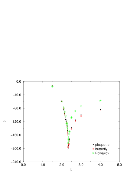
FIG. 1.: $\rho$ vs. $\beta$ for different abelian projections. Lattice $12^{3}\times 4$.

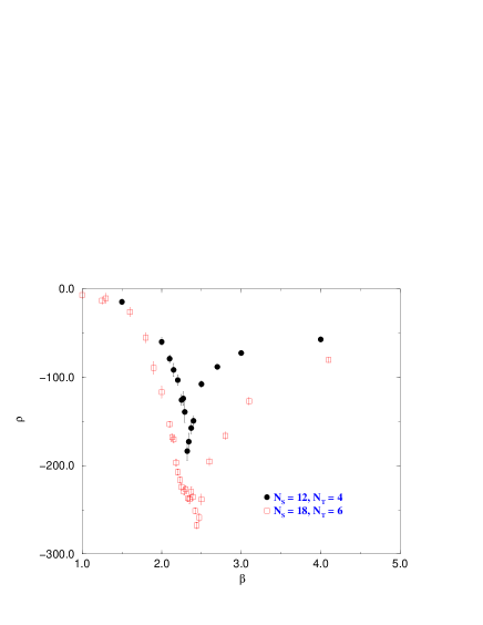
FIG. 2.: $\rho$ vs. $\beta$ for different lattice extensions (lattices $N_{s}^{3}\times N_{t}$). Polyakov projection.

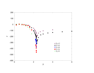
FIG. 3.: $\rho$ as a function of $\beta$ for different spatial sizes at fixed $N_{t}=4$. Plaquette projection.

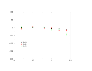
FIG. 4.: $\rho$ vs. $\beta$ in the strong coupling region for lattice sizes $N_{s}^{3}\times 4$. Plaquette projection.

Since different projections give indistinguishable results, for sake of simplicity we shall only display the plaquette projection in the following figures.

Fig. 3 shows the dependence of $\rho$ on $N_{s}$ at fixed $N_{t}=4$. The qualitative behaviour does not change when we increase the lattice size. We now try to understand the thermodynamic limit [6, 12].

In the strong coupling region (cfr. fig. 4) $\rho$ seems to converge to a finite value, which is consistent with $0$ at low $\beta$’s. Eq. (56) then implies that $\langle\mu\rangle\neq 0$ in the infinite volume limit in the confined phase.

The weak coupling region is perturbative. An estimate of $\rho$ is the minimum on the ensemble of the configurations $U$ and is given by the action of classical solutions of the system described by $S+\Delta S$:

$$\rho\mathop{\to}_{\beta\to\infty} \!\!\!\!\!\left[\mathop{\min}_{U}\{S\}-\mathop{\min}_{U}\{S+\Delta S\}\right]$$ (57)

$$= -\mathop{\min}_{U}\{S+\Delta S\}\ ,$$ (58)

since $\mathop{\min}_{U}\{S\}=0$.

In other systems, where the same shifting procedure has been applied and studied, this asymptotic value has been analytically calculated in perturbation theory with the result [6, 12]

$$\rho=-cN_{s}+d\ ,$$ (59)

where $c$ and $d$ are constants, i.e $\rho$ goes linearly with the spatial dimension.

In $SU(2)$ we are unable to perform the same calculation and we have evaluated the minimum $\mathop{\min}_{U}\{S+\Delta S\}$ numerically. Some technical remarks on the numerical procedure. An oversimplified strategy would be to start from a random configuration and then decrease the action by Metropolis-like steps in which the new configuration is accepted only if its action is lower. However this procedure will not work, because of the presence of local minima where often the procedure stops. A way to overcome this difficulty is to perform an usual Monte-Carlo simulation where $\beta$ is increased indefinitively during the simulation [28, 29]. This is equivalent to freeze the system.

We found useful to integrate the two strategies. Firstly we freeze the system increasing $\beta$ in the following way:

1. we thermalize the system at a reasonable $\beta$ (e.g. $\beta=10$);

2. we increase $\beta$ by a fraction $1/200$ and at the new value of $\beta$ we perform a number of sweeps (typically 200), looking for the corresponding minimum of the action;

3. we iterate the step 2 until the minimum of the action looks stable along a larger number of sweeps (typically 5000).

When this procedure becomes inefficient (typically for $\beta\approx 10^{6}$), we go to a Metropolis-like minimization, which is stopped when the action stays constant within errors.

The result is shown in fig. 5 for the plaquette projection. It is consistent with the linear dependence of eq. (59) with $c\simeq 0.6$ and $d\simeq-12$. Thus in the weak coupling region in the thermodynamic limit $\rho$ goes to $-\infty$ linearly with the spatial lattice size and

$$\langle\mu\rangle\mathop{\approx}_{N_{s}\to\infty}Ae^{(-cN_{s}+d)\beta}\to 0,\quad\beta>\beta_{C}\ .$$ (60)

The magnetic U(1) symmetry is restored in the deconfined phase.

FIG. 5.: $\rho$ vs. $N_{s}$ ($N_{t}=4$) at $\beta=\infty$ in the plaquette projection. Data are obtained by numerical minimization of $S+\Delta S$.

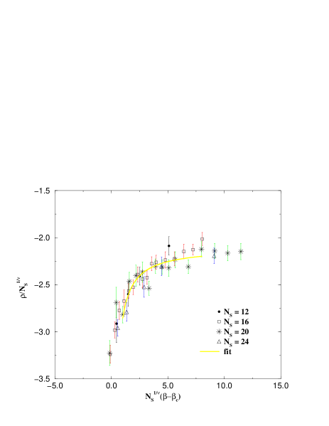
FIG. 6.: Quality of scaling in the plaquette projection at $N_{t}=4$.

To sum up, $\langle\mu\rangle$ is different from zero at least in a wide range of $\beta$ below $\beta_{C}$ and goes to zero exponentially with the lattice size for $\beta>\beta_{C}$. The strong coupling region and the weak coupling one must be connected by a decrease of $\langle\mu\rangle$; the sharp peak of $\rho$ signals that this decline is abrupt and takes place in the critical region.

To understand the behaviour of $\rho$ near the critical point we shall use finite size analysis. By dimensional argument

$$\langle\mu\rangle=N_{s}^{-\delta/\nu}\Phi\left(\frac{\xi}{N_{s}},\frac{a}{\xi},\frac{N_{t}}{N_{s}}\right)\ ,$$ (61)

where $a$ and $\xi$ are respectively the lattice spacing and the correlation length of the system.

Near the critical point, for $\beta<\beta_{C}$

$$\xi\propto\left(\beta_{C}-\beta\right)^{-\nu},$$ (62)

where $\nu$ is the corresponding critical exponent. In the limit $N_{s}\gg N_{t}$ and for $a/\xi\ll 1$, i.e. sufficiently close to the critical point we obtain

$$\langle\mu\rangle=N_{s}^{-\delta/\nu}\Phi\left(N_{s}^{1/\nu}\left(\beta_{C}-\beta\right),0,0\right)$$ (63)

or equivalently

$$\frac{\rho}{N_{s}^{1/\nu}}=f\left(N_{s}^{1/\nu}\left(\beta_{C}-\beta\right)\right)\ .$$ (64)

The ratio $\rho/N_{s}^{1/\nu}$ is a universal function of the scaling variable

$$x=N_{s}^{1/\nu}\left(\beta_{C}-\beta\right)\ .$$ (65)

Since critical values of $\beta$ and critical indices of $SU(2)$ pure gauge theory are well known [27], we can check how well scaling is obeyed by plotting $\rho/N_{s}^{1/\nu}$ as a function of $x$.

Fig. 6 shows the quality of the scaling in the plaquette projection for $\beta_{C}=2.2986$ and $\nu=0.63$. Similar qualitative results have been obtained for the Polyakov projection.

As a further check, we can vary $\nu$ and try to estimate “by eye” sensitivity of our data to this exponent. We obtain that in both projections the scaling relation is satisfied within errors for $0.57\leq\nu\leq 0.67$.

In the thermodynamic limit in some region of $\beta$ below the critical point we expect

$$\langle\mu\rangle\propto\left(\beta_{C}-\beta\right)^{\delta}\ ,$$ (66)

which implies

$$\frac{\rho}{N_{s}^{1/\nu}}=-\frac{\delta}{x}\ .$$ (67)

Using eq. (67) it should be possible in principle to determine $\nu$, $\delta$ and $\beta_{C}$. Our statistic is not enough accurate to perform such a fit. However, we can determine $\delta$ using as an input $\beta_{C}$, $\nu$, which are known, by parameterizing $\rho$ in a wide range by the form

$$\frac{\rho}{N_{s}^{1/\nu}}=-\frac{\delta}{x}-c\ ,$$ (68)

where $c$ is a constant, as suggested by fig. 6.

Our best fit gives $\delta=0.24\pm 0.07$ in the plaquette gauge and $\delta=0.12\pm 0.04$ in the Polyakov gauge. The reduced $\chi^{2}$ is order 1.

This concludes our argument about the thermodynamic limit ($N_{s}\to\infty$). The deconfining phase transition can be seen from a dual point of view as the transition of the vacuum from the dual superconductivity phase to the dual ordinary phase. That feature seems to be independent of the abelian projection chosen.

V The Maximal Abelian projection

There are abelian projections which are not explicitly defined by an operator $\Phi$, but by some extremization procedure. The prototype is the Maximal Abelian projection, which is defined by maximizing numerically the quantity

$$S_{U}(\{\Phi\})=\sum_{n,\mu}\mbox{tr}\left[U_{\mu}(n)\sigma_{3}U^{{\dagger}}_{\mu}(n)\sigma_{3}\right]$$ (69)

with respect to gauge transformations [18, 30].

The Maximal Abelian projection is very popular since, in the projected gauge all links are oriented in the abelian direction within $15\%$, and therefore all observables are dominated by the abelian part within $85\%$. This fact is known as abelian dominance [31], and could indicate that the abelian degrees of freedom in this projection are the relevant dynamical variables at large distances. Moreover, out of the abelian projected configurations, monopoles seem to dominate observable quantities (monopole dominance [32]).

With our approach we have a technical difficulty to determine $\rho$ via $S+\Delta S$ (eq. (38)). At each updating the operator $\Phi$ and $S+\Delta S$ are only known after maximization. Accepting or rejecting an updating therefore requires a maximization, and the procedure takes an extremely long computer time.

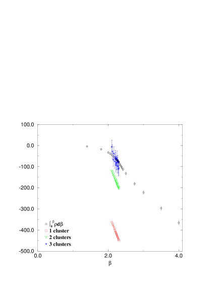
FIG. 7.: $\log\langle\mu\rangle$ reconstruction by cluster expansion. Plaquette projection, lattice $16^{3}\times 4$.

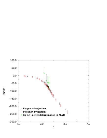
FIG. 8.: $\log\langle\mu\rangle$ in various abelian projections on a $16^{3}\times 4$ lattice.

Therefore in order to study this abelian projection we have to explore the possibility of measuring $\langle\mu\rangle$ directly, and to confront with the huge fluctuations coming from the fact that $\mu$ is the exponential of a sum on a space volume and typically fluctuates as $\sim e^{N_{s}^{3/2}}$. We adopt the following strategy [12]

1. we study the probability distribution of the quantity

   $$\log\mu=-\beta(\Delta S)\ ;$$ (70)

2. we reconstruct $\langle\mu\rangle$ from the $\log\mu$ distribution by means of cumulant expansion formula truncated at some order.

This procedure should be compared with that of ref. [33].

If we have a stochastic variable $X$ distributed with probability $p(X)$ we have

$$\int dXe^{\beta(X-\langle X\rangle)}p(X)=e^{\sum_{n\geq 2}\frac{\beta^{n}}{n!}C_{n}}\ .$$ (71)

$\langle X\rangle$ is the mean value and $C_{n}$ is the $n$-th cluster. For example, if we call $\Delta=X-\langle X\rangle$

$$\begin{array}[]{l}C_{1}=0\ ;\\ C_{2}=\langle\Delta^{2}\rangle\ ;\\ C_{3}=\langle\Delta^{3}\rangle\ ;\\ C_{4}=\langle\Delta^{4}\rangle-3\langle\Delta^{2}\rangle\langle\Delta^{2}\rangle\ ;\\ C_{5}=\langle\Delta^{5}\rangle-10\langle\Delta^{3}\rangle\langle\Delta^{2}\rangle\ .\end{array}$$ (77)

If $\log\mu$ were gaussianly distributed with mean value $m$ and standard deviation $\sigma$, we would have

$$\langle\mu\rangle=\exp\left(m+\frac{\sigma^{2}}{2}\right)\ .$$ (78)

In order to check the method we have explored the cluster expansion for the $\log\mu$ distribution in the projection we have already studied by means of the quantity $\rho$. Fig. 7 shows a comparison between $\log\langle\mu\rangle$, taken from the integration of $\rho$ data, and cluster expansions truncated at different orders. The first and the second cluster are insufficient to account for the right behavior of $\log\langle\mu\rangle$, whereas with the third cluster added the two determinations are consistent. Moreover the fourth cluster is zero within statistical errors. It seems that one can estimate $\langle\mu\rangle$ with a cluster expansion truncated at the third order. As a rule, the higher clusters are quite noisy and error bars grow with increasing order. Therefore this kind of estimation requires a very high statistics. For this reason numerical determination of $\log\langle\mu\rangle$ in the Maximal Abelian projection is possible, but very time consuming. Our data are displayed in fig. 8, showing that monopoles in the Maximal Abelian projection behave in the same way as monopoles in other projections.

For this kind of simulations, we have used a standard overrelaxed heat-bath algorithm. For each value of $\beta$ we performed about 50000 measurements, each of them taken after 8 sweeps. In order to improve the statistics, we have considered eight symmetric different position of the monopole (namely we have inserted the monopole at the center of each optant of a cartesian coordinate system with the origin at the center of the lattice); data corresponding to each position are analyzed separately with the method exposed in the previous section and our best value is the weighted average of the eight measurements. Putting more monopoles would not improve the statistics, since strong correlations appear whenever the distance is shorter than the correlation length. Also these simulations have been performed on a 128-node APE QUADRICS machine.

VI Conclusions

We have constructed a disorder parameter $\langle\mu\rangle$ detecting condensation of monopoles of non abelian gauge theories defined by different abelian projections. The parameter is the vev of an operator which creates a magnetic charge. $\langle\mu\rangle\neq 0$ signals dual superconductivity. The same construction has been tested in many known systems [6, 12, 13].

We measure by numerical simulations $\langle\mu\rangle$, or better $\rho=\frac{\mbox{d}}{\mbox{d}\beta}\log\langle\mu\rangle$, which contains all the relevant informations and less severe fluctuations.

An extrapolation to thermodynamic limit (infinite spatial volume) is possible.

The system behaves as a dual superconductor in the confined phase, and has a transition to normal at the deconfining phase transition, where $\langle\mu\rangle\to 0$.

The deconfining $\beta_{C}$ and the critical index $\nu$ as well as the critical index $\delta$ describing the way in which $\langle\mu\rangle\mathop{\to}0$ when ${T\to T_{C}}$ can be determined. The first two quantities are known independently and our determination is consistent with others. As for $\delta$, defined by

$$\langle\mu\rangle\mathop{\simeq}_{T\to T_{C}}\left(1-\frac{T}{T_{C}}\right)^{\delta}\ ,$$ (79)

it is $0.20\pm 0.08$. Different abelian projections (plaquette, Polyakov, “butterfly”) give results which agree with each other.

Our technique proves difficult for the Maximal Abelian projection, but a direct determination of $\langle\mu\rangle$ looks consistent with other projections.

In conclusions

1. Dual superconductivity is at work in the confined phase, and disappears at the deconfinement phase transition.

2. This statement is independent of the abelian projection defining the monopoles.

Further theoretical effort is needed to understand the real symmetry breaking in the deconfined phase, or in the dual description of QCD.

Similar results for $SU(3)$ will be presented in the companion paper.

Finally we stress that, whatever topological excitations are responsible for colour confinement, counting them is not a right criterion to detect disorder. Only the vev of an operator carrying the appropriate topological charge can be a legitimate disorder parameter.

REFERENCES

- [1] H.V. Kramers, G.H. Wannier, Phys. Rev. 60, 252 (1941).
- [2] L.P. Kadanoff, H. Ceva, Phys. Rev. B3, 3918 (1971).
- [3] G. ’t Hooft, Nucl. Phys. B138, 1 (1978).
- [4] A. Di Giacomo, Prog. Theor. Phys. Suppl. 131, 161-188 (1998).
- [5] N. Seiberg, E. Witten, Nucl. Phys. B426, 19 (1994); Erratum-ibid. B430, 485 (1994).
- [6] G. Di Cecio, A. Di Giacomo, G. Paffuti, M. Trigiante, Nucl. Phys. B489, 739 (1997).
- [7] J. Frölich, P.A. Marchetti, Commun. Math. Phys. 112, 343 (1987).
- [8] V. Cirigliano, G. Paffuti, Commun. Math. Phys. 200, 381 (1999).
- [9] E. Marino, B. Schroer, J.A. Swieca, Nucl. Phys. B200, 473 (1982).
- [10] A. Di Giacomo, Acta Physica Polonica B25, 215 (1994).
- [11] L. Del Debbio, A. Di Giacomo, G. Paffuti, Phys. Lett. B349, 513 (1995).
- [12] A. Di Giacomo, G. Paffuti, Phys. Rev. D56, 6816 (1997).
- [13] A. Di Giacomo, D. Martelli, G. Paffuti, hep-lat/9905007.
- [14] L. Del Debbio, A. Di Giacomo, G. Paffuti, P. Pieri, Phys. Lett. B355, 255 (1995).
- [15] A.M. Polyakov, Nucl. Phys. B120, 429 (1977).
- [16] S. Mandelstam, Phys. Rep. 23c, 245 (1976).
- [17] G. ’t Hooft, in “High Energy Physics”, EPS International Conference, Palermo 1975, ed. A. Zichichi.
- [18] G. ’t Hooft, Nucl. Phys. B190, 455 (1981).
- [19] A. Di Giacomo, Nucl. Phys. Proc. Suppl 47, 136 (1996).
-
[20]
A. Di Giacomo, in Confinement, Duality and Non Perturbative
aspects of QCD, ed. by P. Van Baal, NATO ASI Series B: Physics
Vol. 368, Plenum Press, 415 (1998);
A. Di Giacomo, B. Lucini, L. Montesi, G. Paffuti, Nucl. Phys. Proc. Suppl. 63, 540 (1998);
A. Di Giacomo, B. Lucini, L. Montesi, G. Paffuti, talk presented at Lattice98; to appear on Nucl. Phys. Proc. Suppl.. - [21] G. ’t Hooft, Nucl. Phys. B79, 276 (1974).
- [22] J. Arafune, P.G.O. Freund, G.J. Gobel, Journ. Math. Phys. 16, 433 (1974).
- [23] T.A. De Grand, D. Toussaint, Phys. Rev. D22, 2478 (1980).
- [24] A.S. Kronfeld, G. Schierholz, U.J. Wiese, Nucl. Phys. B293, 461 (1987).
- [25] C.N. Yang, T.D. Lee, Phys. Rev. 87, 404 (1952).
- [26] U.J. Wiese, Nucl. Phys. B375, 45 (1992).
- [27] J. Fingberg, U. M. Heller, F. Karsch, Nucl. Phys. B392, 493 (1993).
- [28] S. Kirckpatrick, C. Gelatt, M. P. Vecchi, Science 220,671 (1983).
- [29] F. Aluffi-Pentini, G. Parisi, F. Zirilli, J. Optim. Theory Appl. 17, 1 (1985).
- [30] A.S. Kronfeld, M.L. Laursen, G. Schierholz, U.J. Wiese, Phys. Lett. B198, 516 (1987).
- [31] T. Suzuki, I. Yotsuyanagi, Phys. Rev. D32, 4257 (1990).
- [32] J. Stack, S. Neiman, R. Wensley, Phys. Rev. D50, 3399 (1994).
- [33] M. N. Chernodub, M. I. Polikarpov, A. I. Veselov, Phys. Lett. B399, 267 (1997).