LA-UR-99-1717 UW-PT/98-15 UTCCP-P-56 DUKE-TH-99-185 Non-perturbative Renormalization Constants using Ward Identities

Abstract

We extend the application of axial Ward identities to calculate $b_{A}$, $b_{P}$ and $b_{T}$, coefficients that give the mass dependence of the renormalization constants of the corresponding bilinear operators in the quenched theory. The extension relies on using operators with non-degenerate quark masses. It allows a complete determination of the $O(a)$ improvement coefficients for bilinears in the quenched approximation using Ward Identities alone. Only the scale dependent normalization constants $Z_{P}^{0}$ (or $Z_{S}^{0}$) and $Z_{T}$ are undetermined. We present results of a pilot numerical study using hadronic correlators.

Wilson’s discretization of the Dirac operator introduces lattice artifacts at $O(a)$, the effects of which are large for lattice spacings accessible in present simulations. It is thus expedient to devise improved lattice discretizations, and significant recent progress has been made in this direction. In particular the ALPHA collaboration has implemented Symanzik’s improvement program [5], in which both the action and external sources are improved by the addition of higher dimensional operators. A key ingredient is the development of methods to determine the coefficients of these extra operators, the “improvement coefficients”, non-perturbatively. In this note we present an extension of these methods which allows the determination of all improvement coefficients for bilinear operators.

We begin by reviewing the results of the ALPHA collaboration. They have shown that $O(a)$ artifacts can be removed from on-shell quantities by the addition of a single local operator of dimension five [6], resulting in the Sheikholeslami-Wohlert (or “clover”) action [7]

$$S = S_{G}+S_{W}+S_{SW}$$ (1)

$$S_{SW} = a^{5}c_{SW}\ \sum_{x}\bar{\psi}(x)\frac{i}{4}\sigma_{\mu\nu}F_{\mu\nu}(x)\psi(x)\,.$$ (2)

Here $S_{G}$ and $S_{W}$ are respectively Wilson’s gluon and quark actions, and $S_{SW}$ is the Sheikholeslami-Wohlert term ($F_{\mu\nu}$ is the lattice gluon field strength tensor). Improvement of quark bilinears is slightly more involved [6]. We consider only flavor off-diagonal operators, the bare lattice forms of which are

$$A^{(jk)}_{\mu} \equiv \bar{\psi^{j}}\gamma_{\mu}\gamma_{5}\psi^{k}\,,$$ (3)

$$V^{(jk)}_{\mu} \equiv \bar{\psi^{j}}\gamma_{\mu}\psi^{k}\,,$$ (4)

$$P^{(jk)} \equiv \bar{\psi^{j}}\gamma_{5}\psi^{k}\,,$$ (5)

$$S^{(jk)} \equiv \bar{\psi^{j}}\psi^{k}\,,$$ (6)

$$T^{(jk)}_{\mu\nu} \equiv \bar{\psi^{j}}i\sigma_{\mu\nu}\psi^{k}\,,$$ (7)

with $j\neq k$ being flavor indices, $\sigma_{\mu\nu}=[\gamma_{\mu},\gamma_{\nu}]/2$, $\gamma_{5}=\gamma_{1}\gamma_{2}\gamma_{3}\gamma_{4}$, and the hermitian $\gamma$ matrices satisfy $\{\gamma_{\mu},\gamma_{\nu}\}=2\delta_{\mu\nu}$. Removal of $O(a)$ errors from the on-shell matrix elements of these bilinears requires both the addition of extra operators (except for $P$ and $S$),

$$(A_{I})_{\mu} \equiv A_{\mu}+ac_{A}\partial_{\mu}P$$ (8)

$$(V_{I})_{\mu} \equiv V_{\mu}+ac_{V}\partial_{\nu}T_{\mu\nu}$$ (9)

$$(T_{I})_{\mu\nu} \equiv T_{\mu\nu}+ac_{T}(\partial_{\mu}V_{\nu}-\partial_{\nu}V_{\mu})\,.$$ (10)

and the introduction of mass dependence,

$$(X_{R})^{(ij)} \equiv Z_{X}^{0}(1+b_{X}am_{ij})(X_{I})^{(ij)}\,.$$ (11)

Here $X=A,V,P,S,T$, the $Z_{X}^{0}$ are renormalization constants in the chiral limit, and $m_{ij}\equiv(m_{i}+m_{j})/2$ is the average bare quark mass.

Complete $O(a)$ improvement of matrix elements requires that the coefficients $c_{SW}$, $c_{X}$, and $b_{X}$, as well as the matching constants $Z_{X}^{0}$, be determined non-perturbatively. Previous work has shown how the enforcement of axial and vector Ward identities (WI) allows one to determine $Z_{V}^{0}$, $Z_{A}^{0}$ and $Z_{P}^{0}/Z_{S}^{0}$ [8], $c_{SW}$, $c_{A}$ and $b_{V}$ [9, 10, 11], $c_{V}$ [12], $c_{T}$ [17], and $b_{P}-b_{A}$ and $b_{S}$ [18]. We discuss here an extension that yields $b_{A}$, $b_{P}$, and $b_{T}$. This provides an alternative to the non-perturbative method proposed in Ref. [17] which uses the short-distance behavior of two point functions. The two remaining constants $Z_{P}^{0}$ (or $Z_{S}^{0}$) and $Z_{T}^{0}$ are scale and scheme dependent, and cannot be determined using WI.

It is important to note that the relations we derive do not extend directly to the unquenched theory, which requires additional improvement constants and a more complicated set of conditions as will be presented in [20].

We begin by recalling the ALPHA method for determining $c_{SW}$ and $c_{A}$ [10]. The improved axial current should satisfy

$$\partial_{\mu}(A_{R})^{(ij)}_{\mu}=(m^{R}_{i}+m^{R}_{j})(P_{R})^{(ij)}+{\cal O}(a^{2})\,,$$ (12)

when inserted between on-shell states. Here $m^{R}$ is the renormalized quark mass. It follows that the ratio

$$2\tilde{m}_{ij} \equiv \frac{\sum_{\vec{x}}\langle\partial_{\mu}[A_{\mu}+ac_{A}\partial_{\mu}P]^{(ij)}(\vec{x},t)J^{(ji)}(0)\rangle}{\sum_{\vec{x}}\langle P^{(ij)}(\vec{x},t)J^{(ji)}(0)\rangle}$$ (13)

$$= (m^{R}_{i}+m^{R}_{j})\frac{Z_{P}^{0}(1+b_{P}am_{ij})}{Z_{A}^{0}(1+b_{A}am_{ij})}\,.$$ (14)

should be independent both of the choice of sources $J$ and of the time $t$, as long as $t\neq 0$, up to corrections of $O(a^{2})$. This is to be achieved by simultaneously tuning $c_{SW}$ and $c_{A}$. Our implementation of this condition differs from the Schrödinger functional method of Ref. [10] in that we use standard two-point correlation functions, with a variety of choices of sources. We also fix $c_{SW}$ a priori and use the condition to determine only $c_{A}$.

It is convenient for the following discussion to introduce $b$ coefficients defined using the masses $\tilde{m}_{ij}$, which we refer to as WI masses, rather than the bare quark mass, i.e.

$$(X_{R})^{(ij)}\equiv Z_{X}^{0}(1+\tilde{b}_{X}a\tilde{m}_{ij})(X_{I})^{(ij)}\,.$$ (15)

The advantage of the WI mass is that it can be determined, using eq. (13), without the need for chiral extrapolation. By contrast, to determine the bare quark mass, $am=1/(2\kappa)-1/(2\kappa_{c})$, one needs to know the critical hopping parameter, $\kappa_{c}$, the calculation of which requires chiral extrapolation. The difference is particularly significant when using standard two-point functions as opposed to the Schrödinger functional. To determine the standard $b_{X}$ from the $\tilde{b}_{X}$ we need the relation between the bare and WI masses, which is given in eq. (32) below. In the quenched theory it follows that

$$b_{X}={Z_{P}^{0}\over Z_{A}^{0}Z_{S}^{0}}\tilde{b}_{X}+O(a)\,.$$ (16)

Note that we only need this relation at leading order in $a$, since the $b_{X}$ appear only in $O(a)$ corrections.

With $c_{SW}$ fixed, $Z_{V}^{0}$ and $\tilde{b}_{V}$ can be obtained in the standard way using charge conservation. We use the forward matrix elements of $(V_{I})_{4}$ between pseudoscalars,

$$\frac{1}{Z_{V}^{0}(1+\tilde{b}_{V}a\tilde{m}_{2})}=$$

$$\hskip 21.68121pt\frac{\sum_{\vec{x},\vec{y}}\langle P^{(12)}(\vec{x},\tau)(V_{I})_{4}^{(22)}(\vec{y},t)J^{(21)}(0)\rangle}{\langle\sum_{\vec{x}}P^{(12)}(\vec{x},\tau)J^{(21)}(0)\rangle}\,.$$ (17)

with $\tau>t>0$ and $J=P$ or $A_{4}$. Here and below we use an abbreviation for the WI mass for two degenerate flavors: $\tilde{m}_{i}=\tilde{m}_{ii}$. Note that the $c_{V}$ term in $V_{I}$ does not contribute to the r.h.s., and so is not determined by this condition.

The remaining improvement constants are determined by enforcing the generic form of the integrated axial WI (AWI), in which the operator ${\cal O}^{23}={\bar{\psi}}^{(2)}\Gamma\psi^{(3)}$ is transformed into $\delta{\cal O}^{13}={\bar{\psi}}^{(1)}\gamma_{5}\Gamma\psi^{(3)}$ by a chiral rotation in the $1,2$ flavor subspace:

$$\biggl{\langle}\delta{\cal S}^{(12)}{\cal O}_{R}^{(23)}(y)J^{(31)}(z)\biggl{\rangle}=\biggl{\langle}\delta{\cal O}_{R}^{(13)}(y)\ J^{(31)}(z)\biggl{\rangle}\,.$$ (18)

Here $\delta{\cal S}$ is the variation in the action

$$\delta{\cal S}^{(12)}=\int_{\cal V}d^{4}x\biggl{[}(m^{R}_{1}+m^{R}_{2})(P_{R})^{(12)}-\partial_{\mu}(A_{R})^{(12)}_{\mu}\biggl{]}\,,$$ (19)

and the chiral rotation is restricted to a 4-volume ${\cal V}$ containing $y$ but not $z$. The Ward identities should hold up to corrections of $O(a^{2})$ if the operators and action are appropriately improved. There is, however, an obstacle to implementing these constraints, arising from the integral over $x$ in $\delta{\cal S}$. This brings the pseudoscalar density $P_{R}(x)$ into contact with the operator ${\cal O}_{R}(y)$ on the l.h.s. of (18), implying that on-shell improvement of $P$ and ${\cal O}$ is insufficient to improve the AWI. (The integral over $\partial_{\mu}A_{\mu}$ gives a surface term which does not involve contact with ${\cal O}$.) The problematic term is explicitly proportional to quark masses, and thus is absent in the chiral limit. For this reason the AWI has previously been used only in the chiral limit, from which one can determine $Z_{A}^{0}$, $Z_{P}^{0}/Z_{S}^{0}$, $c_{V}$ and $c_{T}$, but not the $\tilde{b}_{X}$.

Our new observation is that by looking at the detailed dependence on the quark masses one can work away from the chiral limit and yet avoid contact terms. This allows the determination of certain linear combinations of the $\tilde{b}_{X}$. The cost is the need to use non-degenerate quarks.

For all but the coefficient $\tilde{b}_{T}$, it is sufficient to work with two non-degenerate quarks: $m_{1}=m_{2}\neq m_{3}$. Since the contact term is explicitly proportional to $m_{1}^{R}+m_{2}^{R}$, which itself is proportional to $\tilde{m}_{12}$ at small quark masses, one can remove it by extrapolating to $\tilde{m}_{1}=\tilde{m}_{2}=0$. The remaining $\tilde{m}_{3}$ dependence allows one to determine combinations of the $\tilde{b}_{X}$. In the following, we describe how this works for the different bilinears, and explain our particular implementation. The extrapolation to $\tilde{m}_{1}=\tilde{m}_{2}=0$ will be implicit throughout this discussion.

As a first application we show how to obtain $\tilde{b}_{A}-\tilde{b}_{V}$, as well as $c_{V}$, using the AWI with ${\cal O}=V_{\mu}$. The identity for the time component can be written

$$r_{1} \equiv \frac{\sum_{\vec{y}}\langle\delta{\cal S}^{(12)}_{I}\ (V_{I})_{4}^{(23)}(\vec{y},y_{4})\ J^{(31)}(0)\rangle}{\sum_{\vec{y}}\langle(A_{I})_{4}^{(13)}(\vec{y},y_{4})\ J^{(31)}(0)\rangle}$$ (20)

$$= \frac{Z_{A}^{0}(1+\tilde{b}_{A}a\tilde{m}_{3}/2)}{Z_{A}^{0}\cdot Z_{V}^{0}(1+\tilde{b}_{V}a\tilde{m}_{3}/2)}\,,$$

where $\delta{\cal S}_{I}=-\int_{\cal V}\partial_{\mu}(A_{I})_{\mu}$. For the source we take $J=P$ or $A_{4}$. We have chosen to put the current at $\vec{p}=0$ so that the $c_{V}$ term in $V_{I}$ does not contribute. Since we know $c_{SW}$ and $c_{A}$ we can calculate $r_{1}$, and determine $\tilde{b}_{A}-\tilde{b}_{V}$ from its dependence on $\tilde{m}_{3}$. The intercept provides a determination of $Z_{V}^{0}$ independent of that from eq. (17). The AWI for the spatial components can be written as

$$\tilde{r}_{1} = \frac{\sum_{\vec{y}}e^{i\vec{p}\cdot\vec{y}}\langle\delta{\cal S}^{(12)}_{I}\ [V_{i}+ac_{V}\partial_{\mu}T_{i\mu}]^{(23)}(\vec{y},y_{4})\ A_{i}^{(31)}(0)\rangle}{\sum_{\vec{y}}e^{i\vec{p}\cdot\vec{y}}\langle(A_{I})_{i}^{(13)}(\vec{y},y_{4})\ A_{i}^{(31)}(0)\rangle}\,,$$ (21)

$$= \ r_{1}\,.$$

Enforcing this equality (for any small $\tilde{m}_{3}$) provides a determination of $c_{V}$.

Reversing the roles of vector and axial bilinears provides a second determination of $\tilde{b}_{A}-\tilde{b}_{V}$. For example, if $c_{V}$ is known from above, then one can use the ratio

$$r_{2} \equiv \frac{\sum_{\vec{y}}e^{i\vec{p}\cdot\vec{y}}\langle\delta{\cal S}^{(12)}_{I}\ (A_{I})_{i}^{(23)}(\vec{y},y_{4})\ V_{i}^{(31)}(0)\rangle}{\sum_{\vec{y}}e^{i\vec{p}\cdot\vec{y}}\langle(V_{I})_{i}^{(13)}(\vec{y},y_{4})\ V_{i}^{(31)}(0)\rangle}$$ (22)

$$= \frac{Z_{V}^{0}(1+\tilde{b}_{V}a\tilde{m}_{3}/2)}{Z_{A}^{0}\cdot Z_{A}^{0}(1+\tilde{b}_{A}a\tilde{m}_{3}/2)}\,.$$

Given $Z_{V}^{0}$, this also yields $Z_{A}^{0}$. The same information can be obtained from the combinations

$$\frac{1}{\sqrt{r_{1}\cdot r_{2}}}=Z_{A}^{0}\,,$$ (23)

$$\sqrt{\frac{r_{1}}{r_{2}}}=\frac{Z_{A}^{0}}{Z_{V}^{0}}(1+(\tilde{b}_{A}-\tilde{b}_{V})a\tilde{m}_{3}/2)\,.$$ (24)

Applying the method to the AWI with ${\cal O}=P$ and $S$ gives two determinations of $\tilde{b}_{P}-\tilde{b}_{S}$. For example, one can use the $\tilde{m}_{3}$ dependence of the ratio

$$r_{3} \equiv \frac{\sum_{\vec{y}}e^{i\vec{p}\cdot\vec{y}}\langle\delta{\cal S}^{(12)}_{I}\ S^{(23)}(\vec{y},y_{4})\ J^{(31)}(0)\rangle}{\sum_{\vec{y}}e^{i\vec{p}\cdot\vec{y}}\langle P^{(13)}(\vec{y},y_{4})\ J^{(31)}(0)\rangle}$$ (25)

$$= \frac{Z_{P}^{0}(1+\tilde{b}_{P}a\tilde{m}_{3}/2)}{Z_{A}^{0}\cdot Z_{S}^{0}(1+\tilde{b}_{S}a\tilde{m}_{3}/2)}\,,$$

with $J=P$ or $A_{4}$. Given $Z_{A}^{0}$, this also yields $Z_{P}^{0}/Z_{S}^{0}$. Alternatively, one can use

$$r_{4} \equiv \frac{\sum_{\vec{y}}e^{i\vec{p}\cdot\vec{y}}\langle\delta{\cal S}^{(12)}_{I}\ P^{(23)}(\vec{y},y_{4})\ J^{(31)}(0)\rangle}{\sum_{\vec{y}}e^{i\vec{p}\cdot\vec{y}}\langle S^{(13)}(\vec{y},y_{4})\ J^{(31)}(0)\rangle}$$ (26)

$$= \frac{Z_{S}^{0}(1+\tilde{b}_{S}a\tilde{m}_{3}/2)}{Z_{A}^{0}\cdot Z_{P}^{0}(1+\tilde{b}_{P}a\tilde{m}_{3}/2)}\,,$$

where for the source we choose either $J^{(31)}=S^{(31)}$ or $\sum_{\vec{z}}P^{(34)}(\vec{z},z_{4})P^{(41)}(0)$ for $0<y_{4}<z_{4}$.

The method described so far does not work for the tensor bilinear, because the chiral rotation transforms it back into (other components of) itself, and the dependence on $\tilde{b}_{T}$ cancels. One can, however, use the method to determine $c_{T}$ [17] . For example, the AWI with ${\cal O}=T_{ij}$ at $\vec{p}=0$ and $J=T_{k4}$, can be rearranged into

$$1+ac_{T}\frac{\sum_{\vec{y}}\langle[-\partial_{4}V_{k}]^{(13)}(\vec{y},y_{4})T_{k4}^{(31)}(0)\rangle}{\sum_{\vec{y}}\langle T_{k4}^{(13)}(\vec{y},y_{4})T_{k4}^{(31)}(0)\rangle}$$

$$\hskip 28.45274pt=Z_{A}^{0}\frac{\sum_{\vec{y}}\langle\delta{\cal S}^{(12)}_{I}\ T_{ij}^{(23)}(\vec{y},y_{4})\ T_{k4}^{(31)}(0)\rangle}{\sum_{\vec{y}}\langle T_{k4}^{(13)}(\vec{y},y_{4})\ T_{k4}^{(31)}(0)\rangle}\,,$$ (27)

Here we have moved the $c_{T}$ dependence in $(T_{I})_{k4}$ onto the l.h.s., and used the fact that $(T_{I})_{ij}$ has no contribution from the $c_{T}$ term at $\vec{p}=0$. Given $Z_{A}^{0}$, this equation determines $c_{T}$. A consistency check is that the result should be independent of $\tilde{m}_{3}$.

It turns out that one can determine $b_{T}$ using the AWI (18), but to do so one must work with non-zero $m_{1}$ and $m_{2}$. This means that the AWI is not completely improved: terms of $O(a)$ result from the contact of the pseudoscalar density in $\delta S$ with the operator ${\cal O}$. The key point, however, is that these terms are proportional to $\tilde{m}_{1}+\tilde{m}_{2}$, while the dependence on $b_{T}$ is proportional to the difference $\tilde{m}_{1}-\tilde{m}_{2}$. By separating these two dependences one can, in principle, determine $b_{T}$.

To explain this in detail we recall that off-shell $O(a)$ improvement requires the addition of an extra operator (multiplied by an extra improvement coefficient) for each bilinear [17]. For the pseudoscalar and tensor the required additions are

$$P^{(12)}\longrightarrow P^{(12)} + ac^{\prime}_{P}\bar{\psi}^{(1)}(-\overleftarrow{\mathchoice{{{\hbox to0.0pt{\hbox to8.55695pt{\hss$\displaystyle/$\hss}\hss}\hbox{$\displaystyle D$}}}}{{{\hbox to0.0pt{\hbox to8.55695pt{\hss$\textstyle/$\hss}\hss}\hbox{$\textstyle D$}}}}{{{\hbox to0.0pt{\hbox to5.98985pt{\hss$\scriptstyle/$\hss}\hss}\hbox{$\scriptstyle D$}}}}{{{\hbox to0.0pt{\hbox to4.27846pt{\hss$\scriptscriptstyle/$\hss}\hss}\hbox{$\scriptscriptstyle D$}}}}}+m_{1})\gamma_{5}\psi^{(2)}$$ (28)

$$+ ac^{\prime}_{P}\bar{\psi}^{(1)}\gamma_{5}(\overrightarrow{\mathchoice{{{\hbox to0.0pt{\hbox to8.55695pt{\hss$\displaystyle/$\hss}\hss}\hbox{$\displaystyle D$}}}}{{{\hbox to0.0pt{\hbox to8.55695pt{\hss$\textstyle/$\hss}\hss}\hbox{$\textstyle D$}}}}{{{\hbox to0.0pt{\hbox to5.98985pt{\hss$\scriptstyle/$\hss}\hss}\hbox{$\scriptstyle D$}}}}{{{\hbox to0.0pt{\hbox to4.27846pt{\hss$\scriptscriptstyle/$\hss}\hss}\hbox{$\scriptscriptstyle D$}}}}}+m_{2})\psi^{(2)}\,,$$

$$(T_{I})_{\mu\nu}^{(23)}\longrightarrow(T_{I})_{\mu\nu}^{(23)} + ac^{\prime}_{T}\bar{\psi}^{(2)}(-\overleftarrow{\mathchoice{{{\hbox to0.0pt{\hbox to8.55695pt{\hss$\displaystyle/$\hss}\hss}\hbox{$\displaystyle D$}}}}{{{\hbox to0.0pt{\hbox to8.55695pt{\hss$\textstyle/$\hss}\hss}\hbox{$\textstyle D$}}}}{{{\hbox to0.0pt{\hbox to5.98985pt{\hss$\scriptstyle/$\hss}\hss}\hbox{$\scriptstyle D$}}}}{{{\hbox to0.0pt{\hbox to4.27846pt{\hss$\scriptscriptstyle/$\hss}\hss}\hbox{$\scriptscriptstyle D$}}}}}+m_{2})i\sigma_{\mu\nu}\psi^{(3)}$$ (29)

$$+ ac^{\prime}_{T}\bar{\psi}^{(2)}i\sigma_{\mu\nu}(\overrightarrow{\mathchoice{{{\hbox to0.0pt{\hbox to8.55695pt{\hss$\displaystyle/$\hss}\hss}\hbox{$\displaystyle D$}}}}{{{\hbox to0.0pt{\hbox to8.55695pt{\hss$\textstyle/$\hss}\hss}\hbox{$\textstyle D$}}}}{{{\hbox to0.0pt{\hbox to5.98985pt{\hss$\scriptstyle/$\hss}\hss}\hbox{$\scriptstyle D$}}}}{{{\hbox to0.0pt{\hbox to4.27846pt{\hss$\scriptscriptstyle/$\hss}\hss}\hbox{$\scriptscriptstyle D$}}}}}+m_{3})\psi^{(3)}\,.$$

Inserting the off-shell improved operators into the AWI considered previously we find

$$r_{5} \equiv \frac{\sum_{\vec{y}}e^{i\vec{p}\cdot\vec{y}}\langle\delta{\cal S}^{(12)}_{I}\ (T_{I})_{ij}^{(23)}(\vec{y},y_{4})\ T_{k4}^{(31)}(0)\rangle}{\sum_{\vec{y}}e^{i\vec{p}\cdot\vec{y}}\langle(T_{I})_{k4}^{(13)}(\vec{y},y_{4})\ T_{k4}^{(31)}(0)\rangle}$$ (30)

$$= \frac{1+a\tilde{b}_{T}(\tilde{m}_{1}-\tilde{m}_{2})/2}{Z_{A}^{0}(1-a\tilde{b}_{A}\tilde{m}_{12})}-2a(c^{\prime}_{T}+c^{\prime}_{P})\tilde{m}_{12}\,,$$

Note that both the $\tilde{b}_{A}$ term and the contact terms proportional to $c^{\prime}_{T}+c^{\prime}_{P}$ depend on $\tilde{m}_{12}$. Thus, assuming that $c_{T}$ is known, $\tilde{b}_{T}$ can be obtained from the dependence of $r_{5}$ on $\tilde{m}_{1}-\tilde{m}_{2}$. Note that the ratio $r_{5}$ depends on $c_{T}$ at both zero and non-zero momentum.

A similar extension can be considered for the other AWI discussed above. It is straightforward to see that the $\tilde{m}_{1}-\tilde{m}_{2}$ dependence of the ratios $r_{1}$ and $r_{2}$ allows a determination of $\tilde{b}_{V}+\tilde{b}_{A}$, while that of $r_{3}$ and $r_{4}$ gives a determination of $\tilde{b}_{P}+\tilde{b}_{S}$. Thus, in principle, one can determine all the $\tilde{b}_{X}$ using the generic AWI. One can also determine the five additional improvement constants $c^{\prime}_{X}$ using the dependence on $\tilde{m}_{12}$ as will be discussed in [20]. Further consistency checks are provided by the three-point vector WI with non-degenerate masses—although these by themselves do not allow one to disentangle the $\tilde{b}_{X}$ from the $c^{\prime}_{X}$.

Petronzio and di Divitiis have shown that one can also use the two-point versions of the vector and axial WI to determine a subset of the quenched $b_{X}$, namely $b_{A}-b_{P}$, $b_{S}$ and $b_{V}$ [18]. The key point is again the use of non-degenerate quarks. In our numerical study we use some of their results, which we recall here.

The first result is obtained by comparing the WI mass $\tilde{m}$ to the bare quark mass $m$. These two masses are both related to the renormalized quark mass, the former through eq. (14), and the latter by

$$m_{i}^{R}=Z_{m}^{0}(1+\tilde{b}_{m}a\tilde{m}_{i})\ m_{i}$$ (31)

Combining these relations, and considering only degenerate masses $m_{i}=m_{j}$, one finds

$$\frac{m}{\tilde{m}} = \frac{Z_{A}^{0}}{Z_{P}^{0}Z_{m}^{0}}[1+(\tilde{b}_{A}-\tilde{b}_{P}-\tilde{b}_{m})a\tilde{m}]$$ (32)

$$= \frac{Z_{A}^{0}Z_{S}^{0}}{Z_{P}^{0}}[1+(\tilde{b}_{A}-\tilde{b}_{P}+\tilde{b}_{S}/2)a\tilde{m}]\,.$$ (33)

To obtain the second line we have used the results $Z_{m}^{0}Z_{S}^{0}=1$ and $b_{S}=-2b_{m}$, the latter valid only in quenched QCD [22]. Thus, from the slope and intercept of (33) one can determine $\tilde{b}_{A}-\tilde{b}_{P}+\tilde{b}_{S}/2$ and ${Z_{A}^{0}Z_{S}^{0}}/{Z_{P}^{0}}$, respectively. To use this method we need to determine $\kappa_{c}$, which involves a chiral extrapolation.

The relationship between $\tilde{m}_{ij}$ and $(m_{i}+m_{j})/2$ for non-degenerate quarks gives additional information. It turns out that this information can be gleaned without reference to the bare quark masses, and thus without the need for chiral extrapolation. In particular, by enforcing $(2m_{1})^{R}+(2m_{2})^{R}=2(m_{1}+m_{2})^{R}$ to $O(a)$, one finds

$$\tilde{b}_{P}-\tilde{b}_{A}=-\frac{4\tilde{m}_{12}-2[\tilde{m}_{11}+\tilde{m}_{22}]}{a[\tilde{m}_{11}-\tilde{m}_{22}]^{2}}\,.$$ (34)

This result, in terms of bare masses, was already noted in Ref. [18].

The final result from Ref. [18] uses the vector two-point WI. Requiring $\partial_{\mu}(V_{R})^{(12)}_{\mu}=(m_{1}^{R}-m_{2}^{R})S_{R}^{(12)}$ leads to

$$\Delta_{12} \equiv \frac{\sum_{\vec{x}}e^{i\vec{p}\cdot\vec{x}}\langle\partial_{\mu}{V_{I}}_{\mu}^{(12)}(\vec{x},t)J^{(21)}(0)\rangle}{\sum_{\vec{x}}e^{i\vec{p}\cdot\vec{x}}\langle S^{(12)}(\vec{x},t)J^{(21)}(0)\rangle}$$ (35)

$$= \frac{Z_{S}[1+\tilde{b}_{S}a\tilde{m}_{12}]}{Z_{V}[1+\tilde{b}_{V}a\tilde{m}_{12}]}(m^{R}_{1}-m^{R}_{2})\,.$$ (36)

We implement this using two sources: $J^{(21)}=S^{(21)}$, and $J^{(21)}=\sum_{\vec{z}}P^{(23)}(\vec{z},z_{4})P^{(31)}(0)$ with $0<t<z_{4}$. Enforcing the relation $(2m_{1})^{R}-(2m_{2})^{R}=2(m_{1}-m_{2})^{R}$ to $O(a)$, with the l.h.s. determined from the AWI (14) and the rhs from the vector WI (35), we find

$$\frac{b_{S}-b_{V}}{2}+(b_{P}-b_{A})=\frac{\Delta_{12}-R_{Z}[m_{11}-m_{22}]}{aR_{Z}[m_{11}^{2}-m_{22}^{2}]}\,,$$ (37)

$$R_{Z}\equiv\frac{Z_{S}^{0}}{Z_{P}^{0}}\cdot\frac{Z_{A}^{0}}{Z_{V}^{0}}\,.$$ (38)

We can use eqs. (34,37) to determine $b_{P}$ and $b_{S}$ separately, since $b_{V}$ and $b_{A}$ are already known from eqs. (17,20).

We have performed a pilot test of our method on an ensemble of $16^{3}\times 48$ quenched lattices at $\beta=6/g^{2}=6.0$. We use the tree-level tadpole-improved value for the clover coefficient, $c_{SW}=1.4755$, rather than the non-perturbative value $c_{SW}=1.769$ [10]. This implies that our results for the $b_{X}$ differ from the non-perturbative values by corrections of $O(g^{2})$. We do not have data with three non-degenerate quarks, and so can test only the simpler version of our method which does not yield $b_{T}$. Nevertheless, our results should suffice to assess the practicality of using WI with non-degenerate quarks to determine the $b_{X}$ non-perturbatively.

Previous determinations of the improvement coefficients $c_{X}$ have used Schrödinger functional boundary conditions in the time direction, with sources $J$ placed on the boundaries. One advantage of this approach is that one can work directly in the chiral limit. In our study we use the same correlation functions as used in studying the spectrum and decay constants, i.e. we have periodic boundary conditions in the time direction. Thus a secondary output of our study is a comparison of these two approaches for determining the $c_{X}$. We stress, however, that our method for determining the $b_{X}$ works for any choice of sources $J$, and in particular can be applied to the Schrödinger functional.

The correlation functions required in the integrated axial Ward identity (18) are obtained as follows. Quark propagators are calculated using a Wuppertal smeared source at $t=0$ for five different values of $\kappa$ corresponding to $aM_{\pi}=0.57,0.50,0.43,0.35,0.24$. These propagators are used both to construct two-point functions and also as sources for propagators with the insertion of $\delta S_{I}$ defined in eq. (19). Our insertion volume ${\cal V}$ is the region between $t=4$ and $18$. The second inversion uses the same $\kappa$, so that, as already noted, $m_{1}=m_{2}$. To construct three-point functions, propagators with and without sources are contracted to form the operator ${\cal O}$. This allows us to insert any momentum into ${\cal O}$ and to place it anywhere in the interval $4<t<18$.

For the chiral extrapolations we ignore the correlations in the data between the different mass points. We find poor signals in some of the correlators containing quarks of the lightest mass, and so exclude the lightest mass from the extrapolations. The remaining four values of quark mass correspond to the range $m_{s}-2.6m_{s}$, where $m_{s}$ is the physical strange quark mass. Note that the relevant expansion parameter here is $m_{q}a$, and this is small for our range of quark masses.

Our results from the various WI are summarized in Table 1. Where there is a choice of sources, $J$, we have quoted the results with the best signal. In the following we discuss the various determinations pointing out salient features.

eq.	observable	two-point $\partial$	three-point $\partial$
13	$c_{A}$	$-0.005(15)$	$-0.025(10)$
17	$Z^{0}_{V}$	$+0.745(1)$	$+0.746(1)$
17	$\tilde{b}_{V}$	$+1.57(2)$	$+1.57(2)$
20	$Z^{0}_{V}$	$+0.753(6)$	$+0.759(6)$
20	$\tilde{b}_{A}-\tilde{b}_{V}$	$-0.56(9)$	$-0.48(10)$
21i	$c_{V}$	$-0.66(27)$	$-0.65(25)$
22i	$Z^{0}_{V}/(Z^{0}_{A})^{2}$	$+1.41(12)$	$+1.38(11)$
22i	$\tilde{b}_{A}-\tilde{b}_{V}$	$+1.2(1.2)$	$+1.8(1.0)$
22ii	$c_{V}$	$-0.30(26)$	$-0.31(24)$
23	$Z^{0}_{A}$	$+0.76(2)$	$+0.77(2)$
24	$Z^{0}_{A}/Z^{0}_{V}$	$+0.97(5)$	$+0.98(4)$
24	$\tilde{b}_{A}\!-\!\tilde{b}_{V}$	$+0.38(74)$	$+1.09(69)$
25	$Z^{0}_{A}Z^{0}_{S}/Z^{0}_{P}$	$+0.95(2)$	$+0.98(1)$
25i	$\tilde{b}_{P}\!-\!\tilde{b}_{S}$	$-0.09(9)$	$-0.06(9)$
27	$c_{T}$	$+0.17(7)$	$+0.18(6)$
33	$Z^{0}_{A}Z^{0}_{S}/Z^{0}_{P}$	$+0.97(1)$	$+0.97(1)$
33	$\tilde{b}_{A}\!-\!\tilde{b}_{P}+\tilde{b}_{S}/2$	$+0.48(1)$	$+0.50(1)$
34	$\tilde{b}_{P}\!-\!\tilde{b}_{A}$	$-0.20(9)$	$-0.13(8)$
37	$\tilde{b}_{S}\!-\!\tilde{b}_{V}\!-\!2\tilde{b}_{P}\!-\!2\tilde{b}_{A}$	$+0.04(48)$	$-0.27(38)$

Table 1: Results for improvement coefficients from the listed WI. The two columns of results are for two choices of discretization of derivatives in eq. (13), as discussed in the text. The labels “i”–“v” are explained in the text.

We determine $c_{A}$ by requiring that the right hand side of eq. (13) is as close to a constant as possible over a range of times $t_{\rm min}-t_{\rm max}$. For long times only the pion contributes and the ratio is constant for all values of $c_{A}$—thus any choice of $t_{\rm max}$ in the pion-dominated region is equally good. To maximise our sensitivity to $c_{A}$, we choose $t_{\rm min}$ as small as possible while avoiding contact between $\delta S_{I}$ and $J$. We find that our results are insensitive to small variations in $t_{\rm min}$. There is a similar insensitivity to the choice of source $J$. This is in marked contrast to results from the unimproved action ($c_{SW}=0$) [21] and gives us confidence that our tadpole-improved action has small enough $O(g^{2}a)$ errors that we can carry out our tests.

To estimate the size of $O(a^{2})$ errors (which become $O(a)$ errors in $c_{A}$), we use two choices of discrete derivatives in eq. (13): a scheme based on two-point derivatives,

$$\partial f(x\!+\!1/2) = f(x\!+\!1)-f(x)\,,$$

$$\partial^{2}f(x\!+\!1/2) = {f(x\!+\!2)-f(x\!+\!1)-f(x)\!+\!f(x-1)\over 2}\,,$$

$$f(x\!+\!1/2) = {f(x\!+\!1)+f(x)\over 2}\,,$$

and one based on three-point derivatives,

$$\partial f(x) = (f(x+1)-f(x-1))/2\,,$$

$$\partial^{2}f(x) = f(x+1)-2f(x)+f(x-1)\,.$$

The $O(a^{2})$ correction in the three-point $\partial f$ is four times larger than in the two-point case. The results for $c_{A}$ from these two discretization schemes differ at $O(a)$. As shown in Table 1, this difference is substantial as, unfortunately, are the statistical errors. Because of this difference, we present results for the remaining improvement constants using both choices of $c_{A}$.

Both discretization schemes yield results for $c_{A}$ significantly different from the value $c_{A}=-0.083(7)$ obtained previously at $c_{SW}=1.769$ using the Schrödinger functional [10]. This difference is presumably a combination of $O(g^{2})$ and $O(a)$ effects. We are unable to resolve this discrepancy in this work.

The signal in the vector WI (17) is very good, and provides our best estimates of $Z_{V}$ and $b_{V}$. There is a tiny dependence on $c_{A}$ due to the determination of the quark mass using eq. 13.

We now turn to results from our new method. We use a two-point discretization of the derivative in $\delta S_{I}$ throughout. In Fig. 1 we show our results for the quantity $r_{1}$ which appears in the AWI (20). The data show a linear dependence on $\tilde{m}_{3}$ for our range of masses.

There is a numerical subtlety in the extraction of $\tilde{b}_{A}-\tilde{b}_{V}$. When using eq. 20, we have to make two choices concerning the form of $A_{I}^{(13)}$: whether to discretize it using two- or three-point derivatives; and whether to use the $m$ dependent value of $c_{A}$ obtained from eq. 13, or the chirally extrapolated value. Both choices only effect the result for $\tilde{b}_{A}-\tilde{b}_{V}$ at $O(a)$. In particular, it is straightforward to see that the two options for $c_{A}$ lead to results for $\tilde{b}_{A}-\tilde{b}_{V}$ differing by $\sim aM_{\pi}^{2}/m$ (assuming pion domination of the correlators). Since $M_{\pi}^{2}/m$ is a large scale, perhaps as large as 5 GeV, these differences, although technically of higher order, can be numerically significant. We find that they are only a 15% effect for the two-point discretization of $A_{I}$, but are much larger for the three-point discretization. For this reason we use the two-point discretization. As for the choice of $c_{A}$, we take the chirally extrapolated value, since this is the consistent choice at the order of improvement we are working. This does, however, have the disadvantage of giving poorer plateaus in the ratio $r_{1}$.

The results for $Z_{V}^{0}$ and $\tilde{b}_{A}-\tilde{b}_{V}$ are given in Table 1. $Z_{V}^{0}$ is consistent, at the two $\sigma$ level, with the result from the vector WI, but has much larger errors. $\tilde{b}_{A}-\tilde{b}_{V}$ is determined with a $\sim 20\%$ error.

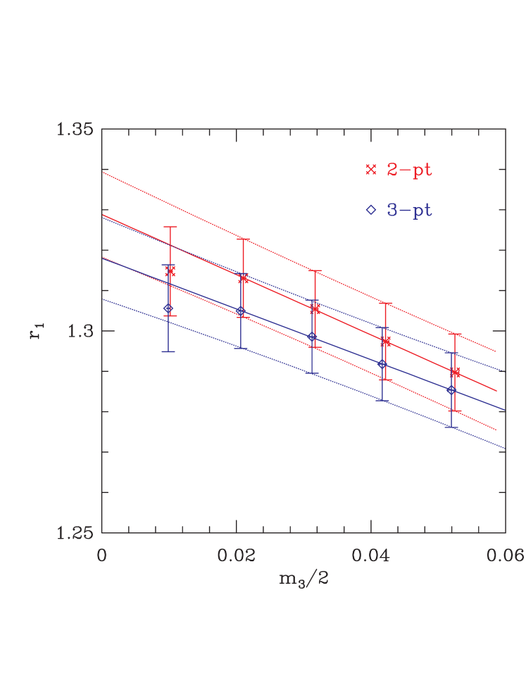
Figure 1: The ratio $r_{1}$ as a function of $\tilde{m}_{3}/2$, after linear extrapolation to $\tilde{m}_{1}=\tilde{m}_{2}=0$. The intercept and slope give $1/Z_{V}^{0}$ and $\tilde{b}_{A}-\tilde{b}_{V}$, respectively. The fit excludes the lightest point as the expected plateau in the fits to the different $r_{i}$ are not uniformly good.

The determination of $c_{V}$ is more problematic and we have attempted a number of approaches. The two best are

• We obtain $c_{V}$ by first equating the right hand sides of Eqs. (20,21) for each $\tilde{m}_{3}$ and then extrapolating to $\tilde{m}_{3}=0$;

• For each $\tilde{m}_{1}=\tilde{m}_{2}$ and $\tilde{m}_{3}$, we solve $r_{1}r_{2}=r_{3}r_{4}$, where only $r_{2}$ depends on $c_{V}$. The chiral extrapolation in $\tilde{m}_{1}=\tilde{m}_{2}$ removes the contribution of the contact terms. Lastly we extrapolate to $\tilde{m}_{3}=0$.

All methods require knowledge of $c_{A}$. The correction term proportional to $c_{V}$ is $\approx 4\%$ in eq. (21) and $\approx 20\%$ in eq. (22), so one needs high statistics to get an accurate estimate. We prefer (i) as it is the most direct, and because $r_{4}$ does not have a good plateau. The large uncertainty in $c_{V}$ extracted by these methods accounts for $\sim 50\%$ of the errors in $Z_{A}^{0}$, and subsequently in $Z_{P}^{0}/Z_{S}^{0}$ and $c_{T}$.

With $c_{V}$ (and $Z_{V}^{0}$) in hand, we use eq. (23) to determine our best estimate of $Z_{A}^{0}$. The results from eqs. (22) and (24) are consistent but have larger errors. The estimates of $\tilde{b}_{A}-\tilde{b}_{V}$ from these two equations have very large errors.

The final application of our new method is the determination of $\tilde{b}_{P}-\tilde{b}_{S}$ using eqs. (25) and (26). Note that neither of these requires knowledge of $c_{V}$. We find a good signal in the ratio $r_{3}$ but not in $r_{4}$. The former is shown in Fig. 2 and the slope yields the value quoted in the table. The intercept gives an estimate of $Z_{P}^{0}/Z_{S}^{0}Z_{A}^{0}$.

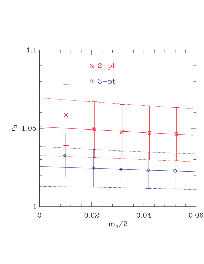
Figure 2: The ratio $r_{3}$ as a function of $\tilde{m}_{3}/2$, after linear extrapolation to $\tilde{m}_{1}=\tilde{m}_{2}=0$. The intercept and slope give $Z_{P}^{0}/(Z_{S}^{0}Z_{A}^{0})$ and $\tilde{b}_{P}-\tilde{b}_{S}$, respectively. The fit excludes the lightest point.

The last mixing coefficient $c_{T}$ is determined from eq. (27). There is a good signal in all correlation functions and only $c_{A}$ and $Z_{A}^{0}$ are needed beforehand. The error is dominated by the uncertainty in $c_{V}$ which feeds in through $Z_{A}^{0}$.

Further information, and consistency checks on the previous results, are provided by the WI using two-point functions. Equation (33) gives a result for $Z_{P}^{0}/Z_{S}^{0}Z_{A}^{0}$, consistent with that from above, with similar errors. It also gives a very accurate result for the combination $\tilde{b}_{A}-\tilde{b}_{P}+\tilde{b}_{S}/2$, with little dependence on $c_{A}$. There is, however, an additional uncertainty due to the choice of $\kappa_{c}$. The two remaining equations, (34) and (37), which do not require $\kappa_{c}$, give rather poor determinations. An important technical point is that the $O(a)$ correction in eq. (35) is large when the source $J^{(21)}$ is chosen to be $S^{(21)}$ as $M_{scalar}a\approx 1$. In order to get results consistent with those from the choice $J^{(21)}=\sum_{\vec{z}}P^{(23)}(\vec{z},z_{4})P^{(31)}(0)$, we needed to use a five-point discretization of $\partial_{\mu}V_{\mu}$ when using the source $J^{(21)}=S^{(21)}$.

	LANL	ALPHA	Pert. Th.
$C_{SW}$	1.4755	1.769	$+1$
$Z^{0}_{V}$	$+0.745(1)(1)$	0.7809(6)	$+0.810$
$Z^{0}_{A}$	$+0.76(2)(1)$	0.7906(94)	$+0.829$
$Z^{0}_{P}/Z^{0}_{S}$	$+0.77(4)(1)$	N.A.	$+0.949$
$c_{A}$	$-0.005(15)(20)$	$-0.083(5)$	$-0.013$
$c_{V}$	$-0.66(27)(02)$	$-0.32(7)$	$-0.028$
$c_{T}$	$+0.17(7)(1)$	N.A.	$+0.020$
$\tilde{b}_{V}$	$+1.57(2)(1)$	N.A.	$+1.106$
$b_{V}$	$+1.62(3)(1)$	1.54(2)	$+1.273$
$\tilde{b}_{A}-\tilde{b}_{V}$	$-0.56(9)(8)$	N.A.	$-0.002$
$\tilde{b}_{P}-\tilde{b}_{S}$	$-0.09(9)(3)$	N.A.	$-0.066$
$\tilde{b}_{P}-\tilde{b}_{A}$	$-0.20(9)(7)$	N.A.	$+0.002$
$\tilde{b}_{A}-\tilde{b}_{P}+\tilde{b}_{S}/2$	$+0.48(1)(2)$	N.A.	$+0.584$
$b_{A}-b_{P}+b_{S}/2$	$+0.49(2)(2)$	N.A.	$+0.673$
$\tilde{b}_{A}$	$+1.01(09)(09)$	N.A.	$+1.104$
$\tilde{b}_{P}$	$+0.81(14)(16)$	N.A.	$+1.105$
$\tilde{b}_{S}$	$+0.90(17)(13)$	N.A.	$+1.172$

Table 2: Our best estimates for normalization and improvement coefficients, compared to previous results where available, and to tadpole improved 1-loop perturbation theory (using $u_{0}=0.8778$). An estimate of the perturbative errors is $\alpha_{s}^{2}\sim 0.02$. The first error is statistical, the second an estimate of the $O(a^{2})$ error. See text for details.

We collect our best results in Table 2. These are obtained using the two-point derivative in $\delta S_{I}$. The difference between two- and three-point discretization is added as an additional error. Our results are compared to previous non-perturbative results, and to those of tadpole-improved 1-loop perturbation theory. The latter are obtained using 1-loop results available in the literature [13, 14, 15, 16]. We note that for the $c_{X}$ and the $\tilde{b}_{X}$ tadpole improvement is equivalent to using the boosted coupling $g^{2}/u_{0}^{4}$ in the 1-loop result. The same is not true for the $Z_{X}$ and $b_{X}$. The conversion factor between the two definitions of the mass-dependent improvement coefficients, $\tilde{b}_{X}/b_{X}=Z_{A}^{0}Z_{S}^{0}/Z_{P}^{0}$, turns out to be very close to unity (see Table 1). Thus, with the exception of $b_{V}$ and $b_{A}-b_{P}+b_{S}/2$, which are determined quite accurately, we do not convert our results back to the standard definition $b_{X}$.

We draw the following conclusions. First, the method we have introduced appears to have practical utility. In the best channels, the statistical and systematic errors in the determination of the differences $\tilde{b}_{A}-\tilde{b}_{V}$ and $\tilde{b}_{P}-\tilde{b}_{S}$ are small compared to the values, $\tilde{b}_{X}\approx 1$, of the coefficients themselves. Second, $c_{V}$ is determined rather poorly using our WI, and this accounts for a substantial fraction of the errors in $Z_{A}^{0}$, $Z_{P}^{0}/Z_{S}^{0}$, and $c_{T}$. For $c_{A}$ and $c_{V}$, the Schrödinger functional method [9, 10, 11, 12] gives results with much smaller errors. Third, we have found, in some cases, substantial disagreement between the perturbative predictions and our non-perturbative results. The most striking cases are $b_{V}$ and $b_{A}-b_{V}$. These differences could be effects of $O(a^{2})$, and we intend to investigate this issue by repeating the calculations at different values of $a$. Finally, there are also differences between our results and those of the ALPHA Collaboration. We anticipate that these differences are due in part to our use of an action that is not fully $O(a)$ improved. We have initiated simulations at $c_{SW}=1.769$ to verify this.

We acknowledge the support of the Advanced Computing Laboratory at Los Alamos. This work was supported in part by the U.S. Department of Energy grants DE-LANL-ERWE161, DE-FG02-96ER40945, and DE-FG03-96ER40956. SS is very grateful to the Center for Computational Physics at the University of Tsukuba for the hospitality received there while completing this work.