Phase diagram and Debye mass in thermally reduced QCD

Abstract

At temperatures well above the transition QCD admits a thermally reduced version in 3D, which reproduces the long distance physics. We analyze the phase diagram, point out the relevance of Z(3) symmetry in the location of the transition and suggest a way out to reconcile this with the data. Related to this symmetry is the existence of an observable, the Z(N) wall, or rather its 3D version, and discuss some of its advantages over other observables.

1 Introduction

One of the main challenges of thermal QCD is to get reliable numbers. Though the gauge coupling may be small, Linde’s argument[3] tells us that perturbation theory will fail. The powerlike infrared divergencies one meets in perturbation theory will off-set the powers of the coupling constant. At what order in perturbation theory this will happen depends on the observable in question. For the free energy this happens when the static sector starts to dominate, and a simple dimensional argument shows this will happen at $O(g^{6})$. For the Debye mass Linde’s phenomenon starts already at next to leading order. So the problem is certainly not academic! One should bear in mind that Linde’s argument does not deny the existence of a perturbation series. It says that from a certain order on the coefficients are no longer obtained by evaluating a finite number of diagrams of a given loop order.

So we are faced with evaluating non-perturbative effects from the three dimensional sector defined by the static configurations. It was realized some time ago [2] that one could take the static part of the 4D action combined with induced effects by the non-static configurations. This theory gives at large distances the same physics as the 4D theory, and has the advantage of relatively straightforward lattice simulations[6]. In section 2 we discuss the relation between the 4D and the 3D theory. In particular we show how the phase diagram of the 3D theory has a remarkable property: the curve of 4D physics, and the critical curve as determined by perturbation theory do coincide to one and two loop order. However, perturbation theory has no reason to be trustworthy in determining the critical curve, and this is probably the reason why the fit to the numerical determination is problematic.

In section 3 we discuss the physics of the domain wall in some detail.

2 Effective 3D action and symmetry in 4D

Construction of the effective action proceeds along familiar lines. In the case of QCD with $n_{f}$ quarks its form is given by integrating out the heavy modes of $O(T)$:

$$S_{3D}=S_{YM,n=0}+S_{ind}$$ (1)

The first term is the static sector of the pure Yang-Mills theory in 4D with coupling constant $g_{3}=g\sqrt{T}$.

The second term in eq. 1 must contain the symmetries of the original QCD action, as long as they are respected by the reduction process.

So we expect the induced action to be of the form:

$$S_{ind}=V(A_{0})+\mbox{ terms involving derivatives}$$ (2)

$V(A_{0})$ should be invariant under static gauge transformations, C, CP ($A_{0}\to-A_{0}^{T}$) and this reduces it to a sum of traces of even powers of $A_{0}$:

$$V(A_{0})=m^{2}TrA_{0}^{2}+\lambda_{1}(TrA_{0}^{2})^{2}+\lambda_{2}TrA_{0}^{4}+....$$ (3)

Only one independent quartic coupling survives for SU(2) and SU(3). We take it to be ${TrA_{0}^{2}}^{2}$. Note that we lost a symmetry present in the 4D action for gluons alone, and less and less conserved when quarks get lighter and lighter: Z(N) symmetry.

Remember from the lattice formulation of pure Yang-Mills that one can multiply at a given time slice in the original 4D action all links in the time direction with a factor $\exp{\pm i\ {2\pi\over 3}}$. This will not change the form of the action, but will change by the same factor the value of the Wilson line $P$ wrapping around the periodic time direction:

$$P(A_{0})={\cal{P}}{\exp{i\int A_{0}d\tau}}$$ (4)

Clearly in eq. 3 this symmetry has gone. Apparently the reduction process does not respect $Z(3)$ symmetry! The reason for this is twofold:

i)the reduction process does not include the static modes.

ii)the values of $A_{0}/T$ in the effective action are order $g$, whereas the Z(N) symmetry equates the free energy in $A_{0}/T$ and $A_{0}/T+O(2\pi/3)$.

To understand this better – and to prepare the way for the discussion of the domain wall observable in the last section 3 – we recall some familiar facts in 4D for SU(3).

2.1 Z(3) symmetry and domain walls in 4D gauge theory

The free energy $U$ as a function of the Wilson line invariants $TrP,TrP^{2}$ is naturally defined through:

$$\exp{-{VU(t_{1},t_{2})\over T}}=\int DA_{0}D\vec{A}\ \delta(t_{1}-\overline{TrP})\delta(t_{2}-\overline{TrP^{2}})\ \exp{-{S(A)\over{g^{2}}}}$$ (5)

where $\overline{TrP}$ is the normalized space average of the trace over the volume $V$. A natural parametrization of the parameters $t_{1}$ and $t_{2}$ suggests itself: define the phase matrix $\exp{iC}$ with $C$ being a traceless diagonal 3x3 matrix with entries $C_{i}\ ,(i=1,2,3)$ and $\sum_{i}C_{i}=0$, because we have SU(N), not U(N).

Consider pure Yang-Mills. A gauge transformation that is periodic modulo a phase in Z(3) will only change the arguments in the delta functions in eq. 5. Hence the potential $U$ has degenerate minima in all points of the C-plane, where $\exp{iC}=1$, or $\exp{\pm i2\pi/3}$. This is called Z(3) symmetry (and the degeneracy is lifted by the presence of quarks).

This statement is independent of perturbation theory. In fact the potential in eq. 5 has been computed in perturbation theory including two loop order. And this potential includes the static modes. Propagators acquire a mass proportional to the phases $C$, because it acts like a VEV of the adjoint Higgs $A_{0}$.

Hence, for small $C$, eventually Linde’s argument will apply and the perturbative evaluation becomes impossible.

For SU(3) the direction in which the Wilson line phase causes minimal breaking is in the hypercharge direction $C={1\over 3}diag(q,q,-2q)$. Minimal breaking means the maximal number of unbroken massless excitations, that do not contribute to the potential. Hence this is at the same time the valley through which the system tunnels from one minimum to the next. In this ”q- valley” the combined 1 and 2 loop result is exceedingly simple:

$$U^{(1)}+U^{(2)}={4\pi^{2}\over 3}T^{4}(N-1)\left(1-5{g^{2}N\over{(4\pi)^{2}}}\right)q^{2}(1-q)^{2}$$ (6)

For use in the reduced theory we isolate the static part of the one and two loop contribution in the q-valley from eq. 6:

$$\left(U^{(1)}+U^{(2)}\right)_{(n=0)}=-T^{4}(N-1){4\pi^{2}\over 3}\left(2q^{3}+3{g^{2}N\over{(4\pi)^{2}}}q^{2}\right)$$ (7)

Note that the two loop contribution is quadratic in q in contrast to the one loop which is cubic. The two-loop cubic part in eq. 6 comes from a combination of static and non-static modes.

If we prepare the 4D system conveniently this symmetry will give rise to domain walls. Profile and energy of these wall have been computed semi-classically a long time ago[14]. The method of twisted boundary conditions triggers walls and is most economic computerwise. We will discuss them in the context of the lattice formulation in section 3. Be it enough to mention that these boundary conditions force the Wilson lines to change by a Z(N) phase in going from one side to another side of the volume in some a priori fixed space direction. This will trigger a wall profile for the loop in this direction.

It is the long range behaviour of this profile that contains the information on the Debye mass. To one loop order this behaviour comes entirely from the slope of the potential, see above. But to two loop order we have to take the one-loop renormalization of the gradient part of the Wilson line phase into account, and this suffers the Linde effect: there is an infinity of many-loop diagrams contributing to the gradient part. So to next to leading order there are already non perturbative effects in the long range tail of the wall, and hence in the Debye mass, as we mentioned earlier.

On the other hand we know that the effective 3D action correctly reproduces the large distance behaviour of the 4D theory. So a 3D projection of the twist should produce a wall with the same tail as the 4D one. The inside of the wall in both formulations may be quite different but the inside is anyway computable by perturbation theory.

2.2 3D action and 4D physics

The parameters of the 3D theory ($m^{2}$ and $\lambda\equiv\lambda_{1}+\lambda_{2}$ for SU(3)) in eq. 3 can be calculated in perturbation theory by integrating out all modes in a path integral except the mode $A_{\mu}(\vec{x},n=0)$. To one loop order we have the well known result for the Debye mass and for the four point coupling $\lambda$. All higher order terms have a coefficient zero [9]. To two loop order one has to take care not only of the two loop graphs, but also of the 1-loop renormalization of the three dimensional gauge coupling $g_{3}$ and the renormalization of the $A_{0}$ field in the gradient terms. The latter renormalization is taking care of gauge dependence in the two loop graphs.

The result [8] in the $\overline{MS}$ scheme is that both parameters are expressed in the renormalized 4D coupling $g(\mu)$ where $\mu$ is the subtraction point. Eliminating the 4D coupling gives for the dimensionless quantities $x\equiv{\lambda\over{g_{3}^{2}}}$ and $y={{m^{2}}\over{g_{3}^{4}}}$ the result for N=3:

$$xy_{4D}={3\over{8\pi^{2}}}(1+{3\over 2}x)$$ (8)

whereas for N=2:

$$xy_{4D}={2\over{9\pi^{2}}}(1+{9\over 8}x)$$ (9)

Note the absence of explicit $\mu$ dependence in this relation. The variable $x$ has a $\mu\over T$ dependence such that as T becomes large $x$ becomes small.

In conclusion, it is along this line that we have to simulate the 3D system, in order to get information about the 4D theory. Before we do this, we still have to settle an important question: where are – in the $xy$ versus $x$ diagram – possible phase transitions?

2.3 Phase diagram of the 3D theory

To get the phase diagram we must first decide what order parameters to take. In the case of SU(3) there are two: $TrA_{0}^{2}$ and $TrA_{0}^{3}$. Strictly speaking, only the latter is an order parameter, since it flips sign under C. We will study the analogue of eq.5:

$$\exp{-VS_{eff}(D,E)}=\int DA\delta\left(g_{3}^{2}D-\overline{TrA_{0}^{2}}\right)\delta\left(g_{3}^{3}E-\overline{TrA_{0}^{3}}\right)\exp{-S}$$ (10)

Again as for the Wilson line we parametrize D and E in terms of $D=Tr\left[C^{2}\right]$ and $E=Tr\left[C^{3}\right]$ respectively. Let us first state the result one gets for $S_{eff}$ to one and two loop order:

$$S_{eff}={U(n=0)\over T}\hskip 28.45274pt\hbox{one and two loop only}$$ (11)

The one and two loop result equals the static part of the 4D Z(3) potential,eq. 5! This static part was explicitely written in the q-valley, eq.7. It has to be added to the tree result and one gets in terms of the dimensionless variables x and y for N= 2 or 3 colours, absorbing a factor $2\pi$ in q:

$${S_{eff}\over{g_{3}^{6}}}=y\left({N-1\over N}\right)q^{2}+x\left({N-1\over N}\right)^{2}q^{4}-(N-1)\left({1\over{3\pi}}q^{3}+{N\over{(4\pi)^{2}}}q^{2}\right)$$ (12)

The question is now: for what values of x and y we have degenerate minima for q? Keeping only the 1 loop result cubic in q we see that it must be of the order of magnitude of the quartic term of the tree result to get a second degenerate minimum. So q must be of $O({1\over x})$ in that minimum. Thus the quadratic two loop result contributes $O(x)$ less.

From eq.12 we find the potential develops two degenerate minima for N=3 when:

$$xy_{c}={3\over{8\pi^{2}}}(1+{3\over 2}x)$$ (13)

For N=2:

$$xy_{c}={2\over{9\pi^{2}}}(1+{9\over 8}x)$$ (14)

This is important: slope and intercept of the physics line 8 are identical with those of the critical line 13, at least if we can take the low order loop results for the critical line seriously. This was numerically found in ref.[13, 8] The intercept equality is just due to the Z(N) potential in 4D and the effective potential $S_{eff}$ in 3D being identical to one loop. But to two loop order this simple explanation is no longer true. The cubic term in eq.6 is appearing also in the two loop result, but not in the two loop result for the 3D effective action. It is however true that also in 2 loops the leading contribution is the static part of the Z(N) potential, eq.7.

2.4 Saddle point of the effective potential in 3D

In this subsection we will investigate in more detail the computation of the 3D effective potential. The saddle point is found by admitting $A_{0}$ fluctuates around a diagonal and constant background B:

$$A_{0}=B+Q_{0}$$ (15)

whereas the spatial gauge fields fluctuate around zero:

$$A_{i}=Q_{i}.$$ (16)

One then goes through the usual procedure of expanding the effective action 10. The equations of motion fix the background B to be equal to the matrix C, and the part quadratic in the fluctuations will not contain any reference to the Higgs potential $V(A_{0})$. This is clear because the quadratic constraint tells the mass term not to fluctuate. Only the Higgs component parallel to C , $TrCQ_{0}$, has a mass term due to the Higgs potential, $4\lambda TrC^{2}$. So apart from this the quadratic part comes entirely from the static part of the 4D action. We can make a convenient gauge choice, namely the static form of the covariant gauge fixing:

$$S_{gf}=Tr\left([ig_{3}B,Q_{0}]+\partial_{k}Q_{k}\right)^{2}$$ (17)

This gives propagators which are precisely the static version of the propagators appearing in the Wilson line potential 5. Only the component $Q_{0}$ parallel to C is the exception: its propagator has a mass from the Higgs potential and can be written as the the sum of the static propagator and a remaining part (“massive”) containing the mass term:

$${1\over{\vec{p}}^{2}}+{1\over{\vec{p}}^{2}+4\lambda TrC^{2}}-{1\over{\vec{p}}^{2}}$$ (18)

The static propagator dominates in diagrams over the rest. The massive propagator will give rise to half integer powers of x in the perturbative expansion of the potential; gauge couplings contribute $O(1)$ in dimensionless units, whereas Higgs couplings contribute $O(x)$.

As long as we are interested in intercept and slope of the critical curve, it follows that only the static part of the Feynman rules contributes.

Hence the result 11.

Let’s from now on work in the q-valley where we evaluate the effective action 12.

Then two remarks are crucial:

i)The broken minimum occurs for $q=O(1/x)$. Power counting then reveals that from $O(x^{3/2})$ on an infinite number of diagrams contributes to each order.

ii)From five loop order on, the potential starts to develop poles in $q=0$.

We are bringing this up, because insisting on the low order result 13 and fitting numerically the coefficients of $x^{3/2}$ and higher order gives an unexpected result: the numerical coefficients are orders of magnitude larger[8] than the first two in 13. In fig. 1, taken from ref. [8], the situation is shown. Only for very small x the critical and the 4D physics line are allowed to become tangent. It seems that this constraint affects the quality of the fit. Dropping it altogether necessitates numerical determination of transition points at $x\leq 0.04$.

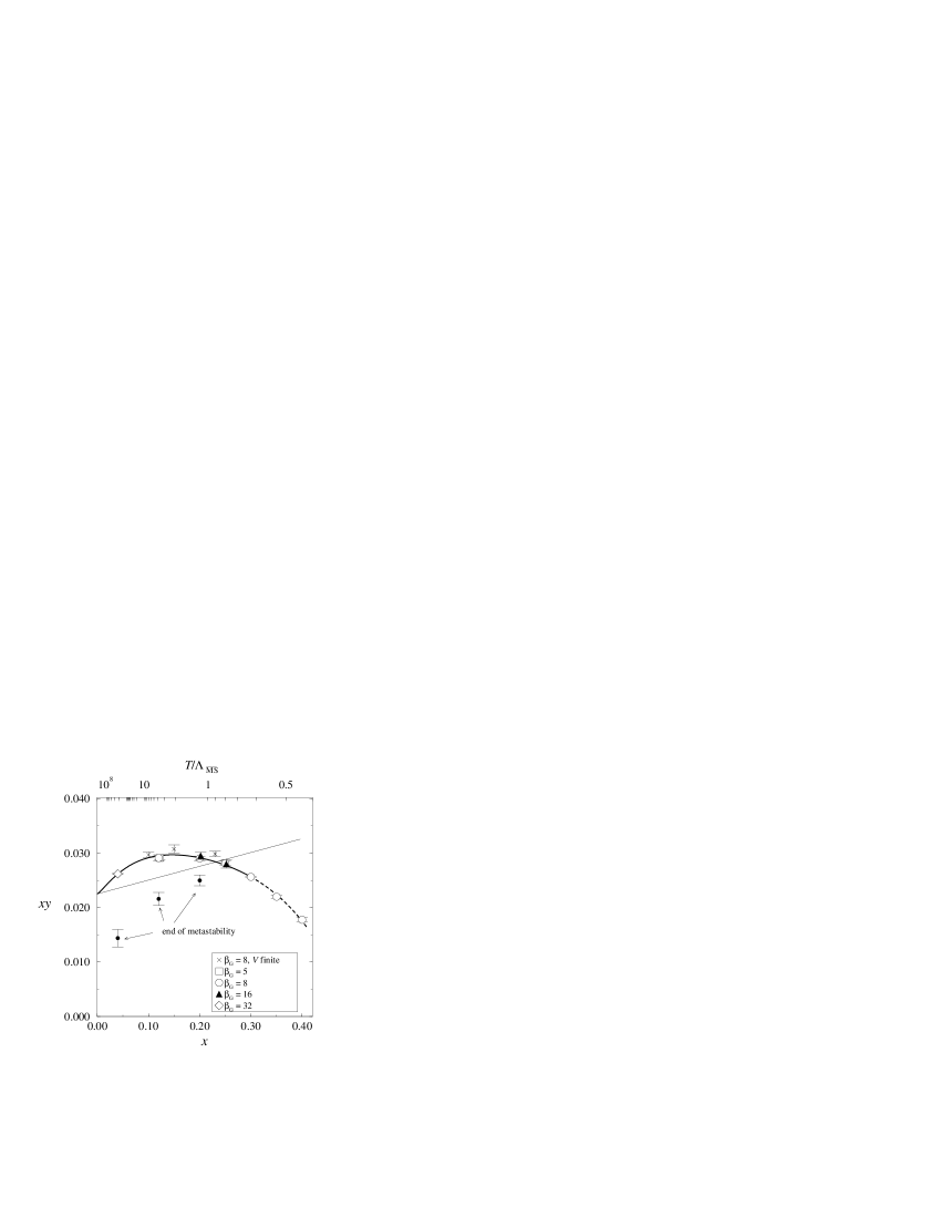
Figure 1: Phase diagram in the SU(2) case, from ref. 9. The straight line is the 4d $\rightarrow$ 3d curve of eq.9. The thick line is a 4th order fit to the data. The dashed line marks the region where the transition turns into a cross-over.

3 Debye mass from a 3D domain wall

After this long discussion of where the physics line lies with respect to the critical curve we have to come to grips with the domain wall method.

The idea here is extremely simple and has been explained elsewhere[11]. Twisted boundary conditions in 4D [16] have a very simple and intuitive form in the reduced theory. Remember that a twisted plaquette in the time-space direction is of the form $Tr(1-\Omega U(P))$, with $\Omega=\exp{i2\pi/N}$.

Thus intuitively one would say that all one has to do in the reduced action is to modify the kinetic part of the Higgs field by the twist, because that’s what the plaquette in the time space direction is reducing to.

In the next subsection we work out this idea in more detail.

3.1 Construction of the wall

In this section we want to make more precise the action that defines the wall.

We follow the notation of ref.[10], specifically that of hep-lat/9811004 and write the kinetic part of the action as:

$${\cal L}_{kin} = {36\over\beta}\sum_{\vec{x}}Tr\left[A^{2}({\vec{x}})\right]\ -\ {12\over\beta}\sum_{{\vec{x}},j}Tr\left[A({\vec{x}})U_{j}({\vec{x}})A({\vec{x}}+a{\vec{e}_{j}})U_{j}^{+}({\vec{x}})\right]$$

$$= {12\over\beta}\sum_{{\vec{x}},j}Tr\left[{1\over 2}\left(A^{2}({\vec{x}})+A^{2}({\vec{x}}+a{\vec{e}_{j}})\right)-A({\vec{x}})U_{j}({\vec{x}})A({\vec{x}}+a{\vec{e}_{j}})U_{j}^{+}({\vec{x}})\right]$$

where $\vec{x}$ is a vector with three components $(x,y,z)$.

Consider the following expression:

$${\cal X}\ =\ 1\ -\ {1\over{\rm N}}{\cal R}e\ Tr\left[e^{{\rm i}\alpha A(x,y,0)}Ue^{-{\rm i}\alpha A(x,y,1)}U^{+}\right]$$

If $\alpha A$ is small we get:

$${\cal X}={1\over{\rm N}}\alpha^{2}Tr\left[{1\over 2}A^{2}(0)+{1\over 2}A^{2}(1)-A(0)UA(1)U^{+}\right]$$

This is precisely the kind of expression that appears in eq. (19). ¿From this follows the expression for the modified kinetic energy in the plane $(x,y,0)$:

$${\cal L}_{kin}^{mod}={12\over\beta}\kern-11.38092pt\sum_{{\vec{x}},j\atop(z,j)\neq(0,3)}\kern-8.5359ptTr\left[{1\over 2}\left(A^{2}({\vec{x}})+A^{2}({\vec{x}}+a{\vec{e}_{j}})\right)-A({\vec{x}})U_{j}({\vec{x}})A({\vec{x}}+a{\vec{e}_{j}})U_{j}^{+}({\vec{x}})\right]$$

$$+\ {12\over\beta}\ {{\rm N}\over\alpha^{2}}\ \sum_{x,y}\left\{1-{1\over{\rm N}}{\cal R}e\ Tr\left[e^{{\rm i}\alpha A(x,y,0)}U_{3}(x,y,0)e^{-{\rm i}\alpha A(x,y,1)}U_{3}^{+}(x,y,0)\right]\right\}$$

So all we need is to put a twist $\Omega\ \in Z({\rm N})\$ in order to get a wall:

$${\cal L}_{kin}^{wall}={12\over\beta}\kern-11.38092pt\sum_{{\vec{x}},j\atop(z,j)\neq(0,3)}\kern-8.82028ptTr\left[{1\over 2}\left(A^{2}({\vec{x}})+A^{2}({\vec{x}}+a{\vec{e}_{j}})\right)-A({\vec{x}})U_{j}({\vec{x}})A({\vec{x}}+a{\vec{e}_{j}})U_{j}^{+}({\vec{x}})\right]$$

$$+{12N\over\beta\alpha^{2}}\sum_{x,y}\left\{1-{1\over{\rm N}}{\cal R}e\left(\Omega\ Tr\left[e^{{\rm i}\alpha A(x,y,0)}U_{3}(x,y,0)e^{-{\rm i}\alpha A(x,y,1)}U_{3}^{+}(x,y,0)\right]\right)\right\}$$

What is now the actual value of $\alpha$ to use? We recover the kinetic term in the continuum if we relate the field $A$ on the lattice to the field $A_{cont}$ in the continuum by the relation:

$$A\ =\ {A_{cont}\over g_{3}}$$

This is not the usual normalization for the lattice fields. Usually we have: $A_{latt}\ =\ ag_{3}A_{cont}$ and $A_{latt}\ \rightarrow\ 0$ in the continuum limit.

Here this is not anymore the case. Remember that to expand the modified action we had to suppose that $\alpha A$ was small. To enforce this condition it seems natural to put : $\alpha\ =\ ag_{3}^{2}$; in this manner terms of the kind $e^{{\rm i}\alpha A}$ become $e^{{\rm i}ag_{3}^{2}A}$. That is to say, they become of the usual sort : $e^{{\rm i}ag_{3}A_{cont}}$.

With this choice the term in the exponential indeed goes to zero as the lattice spacing goes to zero, so:

$$\alpha\ \equiv\ ag_{3}^{2}\ =\ {6\over\beta}$$

In the end we obtain as final expression for the kinetic part of the action supporting the wall:

$${\cal L}_{cin}^{wall}=\displaystyle{12\over\beta}\kern-11.38092pt\sum_{{\vec{x}},j\atop(z,j)\neq(0,3)}\kern-8.82028ptTr\left[{1\over 2}\left(A^{2}({\vec{x}})+A^{2}({\vec{x}}+a{\vec{e}_{j}})\right)-A({\vec{x}})U_{j}({\vec{x}})A({\vec{x}}+a{\vec{e}_{j}})U_{j}^{+}({\vec{x}})\right]$$

$$\displaystyle+\beta\sum_{x,y}\left\{1-{1\over{\rm N}}{\cal R}e\left(\Omega\ Tr\left[e^{{\rm i}{6\over\beta}A(x,y,0)}U_{3}(x,y,0)e^{-{\rm i}{6\over\beta}A(x,y,1)}U_{3}^{+}(x,y,0)\right]\right)\right\}$$

(22)

3.2 Excitations of the wall

Now the system with the wall is defined by adding the 3D gauge field action and the Higgs potential V(A) to eq. 22. Let us call the resulting twisted action $S_{t}$.

Both twisted and untwisted action have periodic boundary conditions. When we compute the average of an observable $O$ in the twisted box we average the observable over the $(x,y)$ plane at the point $z$, written as $\overline{O(z)}$, and compute in the twisted box (action $S_{t}$). It is quite trivial to relate this average to the correlation of the wall and $O$ in the untwisted box (action $S$):

$$\langle\overline{O(z)}\rangle_{S_{t}}=\langle\exp{-(S_{t}-S)}\overline{O(z)}\rangle_{S}$$ (23)

There is no difference between the two actions except at $z=0$, at the location of the wall.

The twist is C and P odd, but T even. This means we can expect a signal for the Debye mass by taking any observable $O$ C odd (a necessary condition[5]). Whatever operator gives the lowest mass in the correlation 23 is the preferred one. Thus one and the same updating with the twisted box can be used for various operators.

4 Conclusions

Once we know the 4D physics line we can do a simulation of the twisted box with some convenient observable, and measure the mass through eq. 23. Care should be taken, as emphasized by Kajantie et al. [6], that we start in the symmetric phase and then move to the 4D physics line. In so doing we will stay on the physical branch of the hysteresis curve for the mass, that we will meet when crossing the transition curve.

Nethertheless our discussion of the location of the critical curve underlines the importance to know wether the 4D physics line lies for small x in the symmetric phase or in the broken phase.

References

References

- [1] S. Bronoff, R. Buffa, C. P. Korthals Altes, hep-ph/9809452, Contributing paper to the proceedings of the 5th International Workshop on Thermal Field Theories and their Applications, Regensburg, Germany, August 10-14, 1998.
- [2] T.Applequist, R.D. Pisarski, Phys. Rev D 23 (1981) 2305 P. Ginsparg, Nucl. Phys B 170 (1980), 388; L. Karkainen, P. Lacock, D. E. Miller, B. Petersson and T. Reisz, Nucl. Phys B 418 (1994), 3.
- [3] A. D. Linde, Phys. Lett.B96(1980),289.
- [4] A. M. Polyakov, Nucl. Phys. B120(1977),429.
- [5] P. Arnold, L. Yaffe, Phys. Rev. D52 (1995) 7208.
- [6] K. Kajantie, M. Laine, J. Peisa, A. Rajantie, K. Rummukainen and M. Shaposhnikov, Phys. Rev. Lett. 79 (1997) 3130; M. Laine, O. Philipsen, Nucl.Phys.B523, (1998), 267, F. Karsch, M. Oevers, P. Petrecky, hep-lat/9807035.
- [7] S. Bronoff and al., in preparation.
- [8] K. Kajantie, M. Laine, K. Rummukainen, M. Shaposhnikov, Nucl. Phys. B503, 1997, 357.
- [9] S.Bronoff, thesis, and S.Bronoff, R. Buffa and C. P. Korthals Altes, in preparation. This fact was known to M.Laine, private communication.
- [10] F. Karsch, in preparation, P. Boucaud, in preparation. K. Kajantie, M. Laine, A. Rajantie, K. Rummukainen and M. Tsypin, hep-lat/9811004.
- [11] S. Bronoff, C. P. Korthals Altes, hep-lat/9808042.
- [12] W. Buchmuller, Z. Fodor, A. Hebecker, Phys.Lett.B331,131,1994, hep-ph/9403391
- [13] J. Polonyi, S. Vasquez, Phys. Lett. B240,183,1990.
- [14] T. Bhattacharya, A. Gocksch, C.P. Korthals Altes and R. D. Pisarski, Phys. Rev. Lett.66(1991),998, Nucl. Phys.B383(1992),487.
- [15] C.P. Korthals Altes, Nucl. Phys.B420(1994),637.
- [16] J. Groeneveld, J. Jurkiewicz and C.P. Korthals Altes, Physica Scr ipta 23, Nr 5, 1022.