Lattice Fields and Extra Dimensions

Michael Creutz

(creutz@bnl.gov)

Physics Department

Brookhaven National Laboratory

Upton, NY 11973

Abstract

Lattice gauge theory is now well into its third decade as a major subfield of theoretical particle physics. I open these lattice sessions with a brief review of the motivations for this formulation of quantum field theory. I then comment on the recent drive of lattice theorists to include a fictitious “fifth” dimension to treat issues of chiral symmetry and anomalies.

PACS: 11.15.Ha

Keywords: lattice gauge theory, domain-wall fermions

Lattice gauge theory, now a mature subject, continues to attract considerable attention as a first principles “solution” of hadronic physics. The basic formulation goes back to Wilson’s classic 1974 paper[1]. The subject remained fairly quiet until an explosive growth in the early 1980’s. The field is currently dominated by numerical simulations, although there is considerable opportunity for analytical developments. We now have an annual lattice conference, moving around the world and attracting typically over 300 participants.

The goals of the lattice community are indeed grandiose. We are attempting first-principles calculations in non-perturbative field theories. Among the most successful targets are direct calculations of hadronic spectra, weak matrix elements relevant to extracting the parameters of the standard model, and the parameters of a new phase of matter, the quark gluon plasma. The next few talks will expand on these calculations. Here I set the stage with a few comments on the basic formulation, trying to explain why we go to a lattice at all. I then turn to some exciting recent developments driving the community to simulations in more than four space time dimensions.

So, if space is continuous, why do we go to a lattice? This is primarily due to two familiar facts. First is the importance of non-perturbative phenomena in strong interaction physics. Quark confinement is inherently non-perturbative; an interacting theory of hadrons is qualitatively different from a perturbation on free quarks and gluons. Second, quantum field theory is rampant with ultraviolet divergences requiring regularization. The issue is that most cutoff schemes are based on perturbation theory. You calculate Feynman diagrams, and when one is infinite you cut it off. However, Feynman diagrams are perturbation theory. It is the need for a non-perturbative regularization that drives us to the lattice.

If you get nothing else from this talk, remember that the purpose of our space-time lattice is nothing but a non-perturbative cutoff. It is a mathematical trick. On a lattice there is a minimum wavelength, given by the lattice spacing $a$; see Fig. 1. In Fourier space, this corresponds to a maximum momentum of $\pi/a$. The scheme gives a mathematically well defined system, allowing numerical computations. This last point has come to dominate the field, but at a deeper level is secondary to providing a definition of the theory.

I now sketch some of the elegant features of Wilson’s [1] original formulation. The concept of a gauge theory means different things to different people. One way to think of a gauge theory is as a theory of phases. As it travels through space time, a charged particle’s wave function acquires a phase

$$U_{i,j}\sim\exp(i\int_{x_{i}}^{x_{j}}A^{\mu}dx_{\mu})$$ (1)

where the line integral is along the path of the particle. From this point of view, natural lattice variables are phase factors associated with the links along which a quark hops. This approach also makes the generalization to a non-Abelian gauge theory particularly simple; the phases are replaced with unitary matrices. For the strong interactions, on any link connecting nearest neighbors we have a 3 by 3 unitary matrix $U_{ij}\in SU(3)$. See Fig. 2. The size of the matrix, 3, is determined by the empirical spectroscopic fact that there are 3 quarks in a proton.

For dynamics, we need a field strength analogous to $F_{\mu\nu}$ in the continuum. Since this is a generalized curl, we are naturally led to consider small loops. Our basic action is a sum over elementary squares, called“plaquettes”

$$S=\int d^{4}xF^{\mu\nu}F_{\mu\nu}\longrightarrow-{1\over 3}\sum_{p}{\rm ReTr}(U_{p})$$ (2)

where the four sides of a given plaquette are multiplied as in Fig. 3. The variable

$$U_{p}=U_{1,2}U_{2,3}U_{3,4}U_{4,1}$$ (3)

represents the flux through the corresponding plaquette.

Given our variables and action, we want to do quantum mechanics. Here the basic approach is via path integrals. We exponentiate the action and integrate over everything

$$Z=\int(dU)e^{-\beta S}$$ (4)

Since our variables are in a Lie group, it is natural to define $dU$ as the invariant group measure. The parameter $\beta$ defines the bare gauge charge

$$\beta={6\over g_{0}^{2}}.$$ (5)

Numerical simulation has dominated lattice gauge theory for most of its history. The algorithms derive from the mathematical equivalence of our path integral with a partition function in statistical mechanics. In this analogy, the link variables correspond to spins, interacting with a four-spin coupling at a “temperature” $1/\beta$. A computer simulation sweeps through stored configurations of a finite system. With pseudo-random numbers, the program makes random changes biased by the Boltzmann weight. This evolution proceeds towards a set of configurations mimicking “thermal equilibrium”

$$P(C)\sim e^{-\beta S}$$ (6)

What is so enticing about this method is that the computer memory contains the entire configuration; in principle the theorist can measure anything desired. Of course it is not always so simple, Monte Carlo simulations have statistical fluctuations. Theorists are faced with the novel situation of having error bars!

In addition to the statistical errors are several sources of systematic uncertainties. These include finite volume and finite lattice spacing corrections. Furthermore, present algorithms only work efficiently for heavy quarks, requiring quark mass extrapolations. In addition, many simulations make what is called a valence approximation for the quark fields. This neglects feedback of the quark fields on the gluons, saving perhaps two orders of magnitude in computer time.

A full inclusion of dynamical quark fields remains not completely understood. Some problems arise directly from the anti-commuting nature of fermion fields. The path integral is no longer a classical statistical mechanics problem, but involves operator manipulations in a Grassmann space. This complication is usually evaded by integrating the fermionic fields analytically as a determinant via the famous formula [2]

$$Z =\int dA\ d\bar{\psi}d\psi\ \exp(S_{g}+\bar{\psi}(\hbox to0.0pt{\hbox to8.55695pt{\hfil/\hfil}\hss}D+m)\psi)$$ (8)

$$=\int dA\ e^{S_{g}}\ |\hbox to0.0pt{\hbox to8.55695pt{\hfil/\hfil}\hss}D+m|$$

This determinant, however, is of an extremely large matrix, tedious to calculate. While many clever tricks have been developed, existing schemes remain, in my opinion, ugly and awkward.

The fermion issue becomes considerably worse when a chemical potential is present. This is the case for studies of a background baryon density. Then the determinant is not positive-definite, wreaking havoc with Monte Carlo methods. In this case, except for very small systems or special toy models, no viable simulation algorithms are known. This is the primary unsolved conceptual problem in lattice gauge theory.

In addition to the algorithmic issues, fermion fields raise fascinating questions in connection with chiral symmetry. Here the difficulties are intertwined tied with the so called “chiral anomalies” of quantum field theory. Of the extensive recent activity in this area, my favorite approaches involve extending space-time to more than four dimensions, making our 4d world an interface in 5d. I turn to this subject for the remainder of this talk.

To see how these higher-dimensional schemes work, I sneak up on the problem by studying an amusing ladder molecule in an applied field [3]. Consider two rows of atoms connected by vertical, horizontal, and diagonal bonds, as sketched in Fig. 4. On such a lattice, an electron initially placed on one atom will spread through the lattice much like water poured in a cell of a metal ice cube tray (Feynman used this analogy in his Caltech lectures of the mid 60’s). Now apply a magnetic field of strength one half flux unit per plaquette orthogonal to the plane of this molecule. This introduces gauge dependent phases on the bonds; one convention for these factors is shown in Fig. 5.

Through interference effects, the magnetic field inhibits the spreading of an electron’s wave function. One consequence is a pair of special states bound on the ends of the ladder. One corresponding wave function is shown in Fig. 6. A symmetric state is bound on other end; its wave function is obtained by inverting this figure.

Symmetry considerations drive these special states to zero energy. The ends of the chain are symmetric under a flip of the system around an axis parallel to the field; so, the end states must have equal energy $E_{L}=E_{R}$. On the other hand, the overall sign of the Hamiltonian can be flipped in two steps. First make a gauge change by multiplying all fermion operators on the lower side of the ladder by $-1$. This changes the signs of all vertical and diagonal bonds. Then change the signs of the horizontal bonds with a left right interchange of the ladder ends. The overall modification implies $E_{L}=-E_{R}$. The only way both conditions can be true is if the states are at exactly zero energy.

This symmetry argument shows that these zero modes are robust under renormalizations. No fine tuning of bond strengths is required. If the chain is not infinitely long, there can be a small, exponentially suppressed, mixing of these states. This will result in energies $E\sim e^{-\alpha L}$, where the parameter $\alpha$ depends on the details of the bond strengths and $L$ is the length of the chain.

These zero modes lie at the heart of the domain-wall fermion approach [4]. We promote the spinor components of a Dirac field on each space time site into a chain as discussed above. One can imagine the chain extending into a fictitious “fifth” dimension. The “zero modes” are then interpreted as the physical quarks. The basic picture is sketched in Fig. 7. The robust nature of these zero modes means that massless fermions remain so when interactions are turned on. Any mass renormalization is proportional to the bare mass, with no additive contributions. This is precisely the role played by chiral symmetry in the “continuum.”

Going back to the ladder analogy, it is easy to see why these modes are automatically chiral. For this we first create a “device” by joining one such ladder onto the side of another, as illustrated in Fig. 8. In this figure, the side chain is our fifth dimension, while the straight chain represents one of the physical space-time dimensions. We augment the model, replacing the factors of $i$ on the horizontal spatial bonds with $i$ times a Pauli spin matrix. The direction in which a surface mode moves is then determined by the direction of its spin. This device is a helicity separator. For more details, see Ref. [3].

I now remark on the exact symmetries of this domain-wall formalism. The zero modes require a surface to exist. If we were to follow the old Kaluza-Klein [5] picture and curl the fifth dimension up into a circle, they would be eliminated. We must cut the circle somewhere, as in Fig. 9. If the size of the extra dimension is finite, the modes mix slightly. Indeed, this is crucial because otherwise there would be no anomalies.

For two flavors, I can obtain the needed zero modes by cutting the circle twice, as in Fig. 10. Now there is one exact chiral symmetry coming from the fact that the fifth dimension involves two topologically distinct pieces. Following the notation from the figure, the number of $u_{L}+d_{R}$ particles is absolutely conserved, as is $u_{R}+d_{L}$. In more usual notation, the axial-vector current

$$j_{\mu 5}^{3}=\overline{\psi}\gamma_{\mu}\gamma_{5}\tau^{3}\psi$$ (9)

is rigorously conserved, even with finite $L_{5}$. There does, however, remain a small flavor breaking. Since they are different components of the same fields, $u_{L}$ and $d_{R}$ will have an exponentially suppressed mixing. This existence of one rigorous chiral symmetry and a small flavor breaking is reminiscent of Kogut-Susskind [6] fermions; however, now we have the length of the fifth dimension to control the size of the flavor breaking.

This scheme gives two flavors from a single five-dimensional field. This naturally leads to speculations about more zero modes and more complicated manifolds. Could this be a route to the flavor/family structure of the standard model? Fig. 11 sketches a conceptual scheme for obtaining three colors of quark and a lepton from a single field.

The question mark in this figure must involve some mechanism for the baryon decay anomaly of the ’t Hooft process. Also, for gauge invariance, appropriate quantum numbers should be transferred between the various singularities giving the physical fermions. One proposed scheme is sketched in Fig. 12, representing the rendition of the model of [7] as presented in [8].

In conclusion, I hope I have convinced you that the lattice provides a powerful non-perturbative regularization, allowing controlled calculations of hadronic processes. I am occasionally asked if the lattice might actually be real. I don’t particularly like this option, which would lead to an uncomfortable flexability. Requiring a continuum limit should limit physical results to renormalizable field theories. Of course, ultimately experiment will have to decide.

Despite the maturity of the field, old unresolved fermion issues remain. The existing algorithms are rather awkward, and none are known for dealing with a background baryon density. Chiral gauge theories remain controversial, but domain-wall fermions appear to be making progress. Some more speculative questions on which the lattice may eventually shed light are whether mirror species[9], such as massive right handed neutrinos, should exist, and whether true chiral theories must be spontaneously broken, as observed in the standard model.

I hope I have at least amused you about the helpful nature of extra dimensions for chiral symmetry. There is some hope that similar techniques can give natural lattice formulations of super-symmetry; an intriguing scheme [10] has been proposed for a lattice formulation of super-symmetric Yang-Mills theory, where the low energy spectrum has all masses protected from fine tuning. Of course, the use of extra dimensions also suggests connections with the recent activities in string theory. Chiral fermions on higher-dimensional membranes are in much the same spirit as the domain-wall fermion approach.

So, well into its third decade, lattice gauge theory remains a thriving industry. While dominated by numerical work, the field is considerably broader. The unsolved problems, particularly with fermionic fields, show that despite the maturity of the subject we still need new ideas!

Acknowledgement: This manuscript has been authored under contract number DE-AC02-98CH10886 with the U.S. Department of Energy. Accordingly, the U.S. Government retains a non-exclusive, royalty-free license to publish or reproduce the published form of this contribution, or allow others to do so, for U.S. Government purposes.

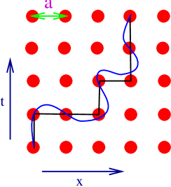
FIG. 1.: Lattice gauge theory approximates quark world-lines by sequences of hops through a four-dimensional lattice. The spacing must be extrapolated to zero for physical results.

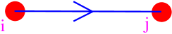
FIG. 2.: On each link connecting two nearest neighbors is a 3 by 3 unitary matrix $U_{ij}\in SU(3)$.

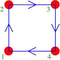
FIG. 3.: Multiplying the phase factors around a plaquette gives the flux through that plaquette. This is used to construct the action.

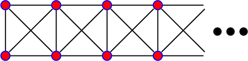
FIG. 4.: The basic ladder molecule discussed in the text.

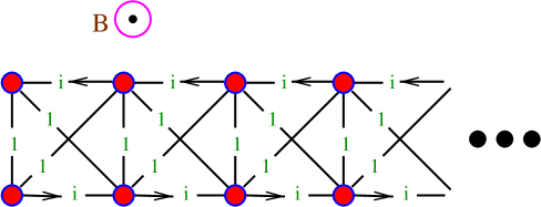
FIG. 5.: Applying a field of one half flux unit per plaquette gives phases on the bonds. One convenient gauge choice is shown here.

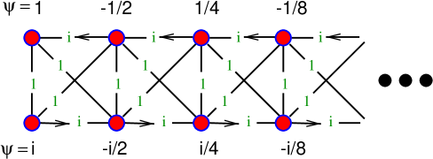
FIG. 6.: The wave function for a zero energy state bound on the end of the ladder molecule.

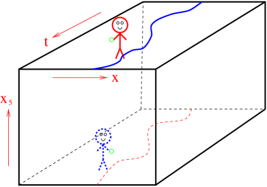
FIG. 7.: For domain-wall fermions, our four-dimensional world is interpreted as a surface on a five-dimensional manifold. Zero modes on this surface are the physical quark degrees of freedom.

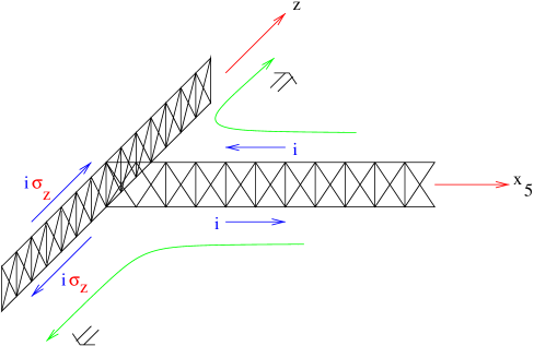
FIG. 8.: A device constructed by joining ladder molecules. Inserting Pauli matrices in the spatial directions creates a helicity filter.

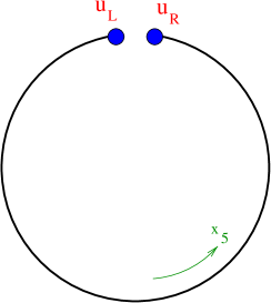
FIG. 9.: A compact fifth dimension must be cut in order to generate the chiral zero modes of the domain-wall formalism.

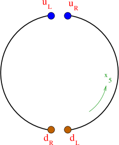
FIG. 10.: Cutting the compact fifth dimension twice gives two flavors of fermion. With the identifications here, one flavored chiral symmetry is exact, even when the lattice spacing and the size of the fifth dimension are finite.

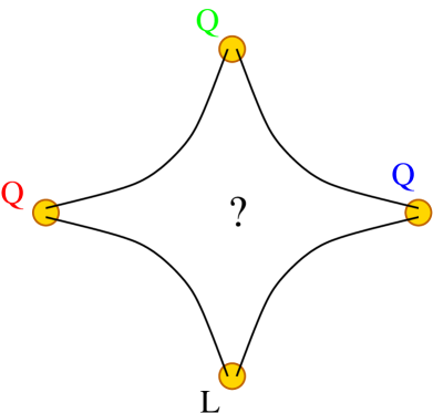
FIG. 11.: Perhaps all fermions in a generation are special modes of a single higher-dimensional field. Here the three quark fields might represent different values of the internal $SU(3)$ symmetry, and $L$ could represent a lepton from the same family.

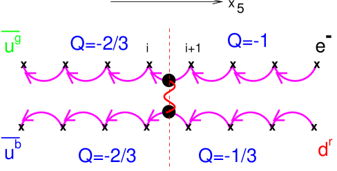
FIG. 12.: One specific model with three quark colors and a lepton all being manifestations of a single five-dimensional fermion field.

REFERENCES

- [1] K. Wilson, Phys. Rev. D10, 2445 (1974).
- [2] P. T. Matthews and A. Salam, Nuovo Cim. 12, 563 (1954).
- [3] M. Creutz, hep-lat/9902028.
- [4] D. Kaplan, Phys. Lett. B288 (1992) 342; V. Furman and Y. Shamir, Nucl. Phys. B439, 54 (1995).
- [5] Th. Kaluza, Sitzungsber. Preuss. Akad. Wiss. Leipzig, 966 (1921); O. Klein, Z. Phys. 37, 895 (1926).
- [6] J. Kogut and L.Susskind, Phys. Rev. D11, 395 (1975).
- [7] M. Creutz, C. Rebbi, M. Tytgat, and S.-S. Xue, Physics Letters B402, 341 (1997).
- [8] M. Creutz, Nuclear Physics B (Proc.Suppl.) 63A-C, 599 (1998).
- [9] I. Montvay, Nucl. Phys. B (Proc. Suppl.) 30, 621 (1993); Phys. Lett. 199B, 89 (1987).
- [10] J. Nishimura, Phys. Lett. B406, 215 (1997); N. Maru, J. Nishimura,Int. J. Mod. Phys. A13 2841 ( 1998); T. Hotta, T. Izubuchi, and J. Nishimura, Mod. Phys. Lett. A13, 1667 (1998).