DESY-99-023

OUTP-99-07P

Hadron masses and matrix elements from
the QCD Schrödinger functional

Marco Guagnelli^a, Jochen Heitger^b, Rainer Sommer^b and Hartmut Wittig^c,
a Dipartimento di Fisica, Università di Roma Tor Vergata
and INFN, Sezione di Roma II
^b DESY-Zeuthen
Platanenallee 6, D-15738 Zeuthen, Germany
^c Theoretical Physics, University of Oxford
1 Keble Road, Oxford OX1 3NP, UK
Abstract

We explain how masses and matrix elements can be computed in lattice QCD using Schrödinger functional boundary conditions. Numerical results in the quenched approximation demonstrate that good precision can be achieved. For a statistical sample of the same size, our hadron masses have a precision similar to what is achieved with standard methods, but for the computation of matrix elements such as the pseudoscalar decay constant the Schrödinger functional technique turns out to be much more efficient than the known alternatives.

March 1999

1 Introduction

In recent years, lattice QCD calculations in the quenched approximation have reached a new quality [?,?,?]. The renormalization of many local composite operators can be treated non-perturbatively, and the leading discretization errors have been removed. Consequently one would now like to perform continuum extrapolations for various hadron masses and matrix elements in the improved theory [?,?,?,?,?,?] and compare to recent results obtained with more standard techniques [?]. In particular, the problem of a determination of the light quark masses can be addressed with confidence, since the complete renormalization is known non-perturbatively [?].

However, continuum extrapolations require masses and matrix elements for finite values of the lattice spacing which are sufficiently accurate [?]. Efficient methods are needed to obtain such precise results. Standard methods use correlation functions in a sufficiently large box with periodic boundary conditions [?]. Usually one seeks to enhance the dominance of the low lying hadrons by using tuned hadron wave functions [?,?,?,?,?,?,?,?,?,?], possibly combined with variational techniques [?,?,?].

In this paper we investigate an alternative to these standard methods. Again we choose a sufficiently large box but impose Dirichlet boundary conditions in time, as they are used to formulate the QCD Schrödinger functional . We shall demonstrate that correlation functions in the Schrödinger functional are dominated by hadron intermediate states at large Euclidean time. Moreover, it is shown that a time extent of 3 fm for the box is sufficient to extract masses and matrix elements. An advantage compared to the standard methods is that the pre-asymptotic decay of Schrödinger functional correlation functions is very slow, which means that a large signal remains at large separations.

In the following, we briefly discuss the foundation of the method (Section 2) and test its applicability in practice in the quenched approximation (Section 3). We also attempt to quantify the efficiency compared to more standard calculations (Section 4). Finally we discuss open questions as well as possible further improvements.

2 Correlation functions at large time separations

We now derive explicit expressions for the representation of Schrödinger functional correlation functions in terms of intermediate physical states. Throughout this section we assume that the lattice Schrödinger functional  is defined using the standard Wilson action as in ref. [?]. In this situation the relations presented here hold exactly. If one considers the ${\rm O}(a)$ improved theory, as we will do later, we cannot derive the equations given in this section directly from the transfer matrix. However, universality implies that the renormalized correlation functions of the improved theory and the unimproved theory agree in the continuum limit. Since the correlation functions considered below are renormalized multiplicatively, their time dependence (bare or renormalized) is given by the expressions derived for the Wilson theory up to lattice spacing effects. For the ${\rm O}(a)$ improved theory this means that all relations derived in this section are valid for physical distances large compared to the lattice spacing (up to corrections of order $a^{2}$).

The correlation functions considered here have been introduced before [?,?,?]. In those references the emphasis was largely on the perturbative regime, which means choosing small extensions of the space-time volume. By contrast, in this work we are interested in the correlation functions for intermediate to large volumes, i.e. extensions which are significantly larger than typical QCD scales. Provided that the pion mass is not too small, such typical QCD scales are of order $1~{}{\rm fm}$.

The QCD Schrödinger functional is defined as the QCD partition function in a cylindrical geometry, i.e. periodic boundary conditions with periodicity length $L$ in three of the four Euclidean dimensions, and Dirichlet boundary conditions in time at the hypersurfaces $x_{0}=0$ and $x_{0}=T$. Its quantum mechanical interpretation has first been discussed for the pure gauge theory [?] and subsequently for the theory with quarks [?]. In these references it was shown that the Schrödinger functional partition function can be written as

$${{\cal Z}}=\langle{\rm f}|{\rm e}^{-T\mathbb{H}}\,\mathbb{P}\,|{\rm i}\rangle\,,$$ (2.1)

with states $|{\rm i}\rangle$ and $|{\rm f}\rangle$ which are given in terms of the boundary values specified at $x_{0}=0$ and $x_{0}=T$, respectively. In the above equation $\mathbb{H}$ denotes the Hamilton operator of QCD formulated on a torus of volume $L^{3}$. More precisely, in the lattice theory it is proportional to the (negative) logarithm of the transfer matrix.

Of course, the same operator describes the correlation functions when the Dirichlet boundary conditions are replaced by periodic boundary conditions in time. The projector $\,\mathbb{P}\,$ projects onto the gauge invariant subspace of the Hilbert space [?,?]; only gauge invariant intermediate states are physical and can contribute.

For our present investigation, we have considered only the case of homogeneous boundary conditions, where the spatial components of the gauge potentials are set to zero at the boundaries and also the fermion boundary fields are taken to vanish. In this case we have $|{\rm i}\rangle=|{\rm f}\rangle=|{\rm i}_{0}\rangle$ and this state carries the quantum numbers of the vacuum. Other choices for the boundary conditions may be of interest as well and can be treated similarly.

As an example we will discuss two specific correlations, which allow for a calculation of the pion mass and decay constant. The generalization to other channels and other matrix elements is straightforward.

We start from the dimensionless fields

$${\cal O}={{a^{6}}\over{L^{3}}}\sum_{{\it\bf y},{\it\bf z}}\bar{\zeta}_{\rm u}({\it\bf y})\gamma_{5}\zeta_{\rm d}({\it\bf z})\,,\quad{\cal O}^{\prime}={{a^{6}}\over{L^{3}}}\sum_{{\it\bf y},{\it\bf z}}\bar{\zeta}\kern 1.0pt^{\prime}_{\rm d}({\it\bf y})\gamma_{5}\zeta\kern 1.0pt^{\prime}_{\rm u}({\it\bf z})$$ (2.2)

and a local composite (gauge invariant) field $X(x)$ (which will have mass dimension three in our applications) to define the gauge invariant correlation functions

$$f_{X}(x_{0}) = -{L^{3}\over 2}\langle X(x)\,{\cal O}\rangle\,,$$ (2.3)

$$f_{1} = -{1\over 2}\langle{\cal O}^{\prime}\,{\cal O}\rangle\,,$$ (2.4)

where the average denotes the usual path integral average and ${\rm u,d}$ are flavour indices. The “boundary quark fields”, $\zeta,\ldots,\bar{\zeta}\kern 1.0pt^{\prime}$, have been discussed in [?]. In the lattice theory, $\zeta$ is given explicitly in terms of the gauge fields connecting hypersurfaces $x_{0}=0$ and $x_{0}=a$ and the quark fields on the hypersurface $x_{0}=a$. Analogous properties hold for the other boundary quark fields. Our choices for $X$ are $X=A_{0}$ (defining, through eq. (2.3), the correlation function $f_{\rm A}$) and $X=P$ (which gives $f_{\rm P}$), where

$$A_{0}(x) = \overline{\psi}_{\rm d}(x)\gamma_{0}\gamma_{5}\psi_{\rm u}(x)\,,$$ (2.5)

$$P(x) = \overline{\psi}_{\rm d}(x)\gamma_{5}\psi_{\rm u}(x)\,.$$ (2.6)

The correlation functions $f_{X}$ have the quantum mechanical representation

$$f_{X}(x_{0})={\cal Z}^{-1}\,{L^{3}\over 2}\,\langle{\rm i}_{0}|{\rm e}^{-(T-x_{0})\mathbb{H}}\,\mathbb{P}\,{\,\mathbb{X}\,}{\rm e}^{-x_{0}\mathbb{H}}\,\mathbb{P}\,|{\rm i}_{\pi}\rangle\,,\;a\leq x_{0}\leq T-a\,,$$ (2.7)

where ${\,\mathbb{X}\,}$ is the corresponding operator in the Schrödinger picture, and the state $|{\rm i}_{\pi}\rangle$ has the quantum numbers of the $\pi^{+}$ with momentum zero. To conclude that eq. (2.7) holds, one only requires that the combination of fields ${\cal O}$, eq. (2.2), has support for $x_{0}\leq a$ and that it carries the quantum numbers of a $\pi^{+}$. The former is guaranteed by the very construction of the boundary fields $\zeta,\bar{\zeta}$ [?]. Furthermore we have

$$f_{1}={\cal Z}^{-1}\,\hbox{$1\over 2$}\,\langle{\rm i}_{\pi}|{\rm e}^{-T\mathbb{H}}\,\mathbb{P}\,|{\rm i}_{\pi}\rangle\,.$$ (2.8)

It is now apparent that (for large separations $x_{0}$ and $T-x_{0}$) the mass of the pion and its decay constant can be extracted. To see this explicitly we insert a complete set of eigenstates of the Hamiltonian,

$$|n,q\rangle\,,\quad n=0,1,\ldots\;,$$ (2.9)

$$\mathbb{H}\,|n,q\rangle=E^{(q)}_{n}|n,q\rangle\,,$$ (2.10)

with normalization $\langle n^{\prime},q^{\prime}|n,q\rangle=\delta_{n,n^{\prime}}\,\delta_{q,q^{\prime}}$. Here the energy levels in the sector of the Hilbert space with internal quantum numbers $q$ are enumerated by $n$. Only quantum numbers $q=\pi$, a shorthand for $(J,P,C,I,I_{3})=(0,-,+,1,1)$, and $q=0$, which denotes vacuum quantum numbers are considered in the following. We do not indicate the momentum of the states $|n,q\rangle$, since both $|{\rm i}_{0}\rangle$ and $|{\rm i}_{\pi}\rangle$ are invariant under spatial translations and only states $|n,q\rangle$ with vanishing (spatial) momentum contribute.

The representations given so far hold for arbitrary $L$, $T$ and $x_{0}$. In this paper, we shall be interested in the special case of the asymptotic behavior of $f_{\rm A}(x_{0}),f_{1}$ for large values of both $x_{0}$ and $T-x_{0}$, while $L$ remains unspecified at this stage. We include the first non-leading corrections but neglect any contributions which are suppressed by terms of order

$$\exp(-TE^{(0)}_{1}),\;\exp(-x_{0}E^{(\pi)}_{1}-(T-x_{0})E^{(0)}_{1}),\;\exp(-(T-x_{0})E^{(0)}_{2})\;{\rm and}\;\exp(-x_{0}E^{(\pi)}_{2})\,,$$

compared to the leading terms in the correlation functions. In this approximation we obtain

$$f_{X}(x_{0}) \approx \hbox{$L^{3}\over 2$}\,\rho\,\langle 0,0|{\,\mathbb{X}\,}|0,\pi\rangle\,{\rm e}^{-x_{0}m_{\pi}}\times\left\{1+\eta_{X}^{\pi}{\rm e}^{-x_{0}\Delta}+\eta_{X}^{0}{\rm e}^{-(T-x_{0})m_{\rm G}}\right\},$$ (2.11)

$$f_{1} \approx \hbox{$1\over 2$}\,\rho^{2}\,{\rm e}^{-Tm_{\pi}}\,,$$ (2.12)

where we have introduced the ratios

$$\rho = {\langle 0,\pi|{\rm i}_{\pi}\rangle\over\langle 0,0|{\rm i}_{0}\rangle},$$ (2.13)

$$\eta_{X}^{\pi} = {\langle 0,0|{\,\mathbb{X}\,}|1,\pi\rangle\langle 1,\pi|{\rm i}_{\pi}\rangle\over\langle 0,0|{\,\mathbb{X}\,}|0,\pi\rangle\langle 0,\pi|{\rm i}_{\pi}\rangle}\,,$$ (2.14)

$$\eta_{X}^{0} = {\langle{\rm i}_{0}|1,0\rangle\langle 1,0|{\,\mathbb{X}\,}|0,\pi\rangle\over\langle{\rm i}_{0}|0,0\rangle\langle 0,0|{\,\mathbb{X}\,}|0,\pi\rangle}\,.$$ (2.15)

The energy difference $m_{\rm G}=E^{(0)}_{1}-E^{(0)}_{0}$ is the mass of the $0^{++}$ glueball and $\Delta=E^{(\pi)}_{1}-E^{(\pi)}_{0}$ is an abbreviation for the gap in the pion channel. As indicated above, we have dropped contributions of higher excited states which decay even faster as $x_{0}$ and $T-x_{0}$ become large.

Considering the special case of $f_{\rm A}$, we find that it is proportional to the matrix element $\langle 0,0|{\,\mathbb{A}_{0}}|0,\pi\rangle$, which is related to the pion decay constant $F_{\pi}$ through

$$Z_{\rm A}\langle 0,0|{\,\mathbb{A}_{0}}|0,\pi\rangle=F_{\pi}m_{\pi}(2m_{\pi}L^{3})^{-1/2}\,.$$ (2.16)

Here, $Z_{\rm A}$ is the renormalization constant of the isovector axial current, and the factor $(2m_{\pi}L^{3})^{-1/2}$ takes account of the conventional normalization of one-particle states (in our convention the experimental value of the pion decay constant is 132 MeV).

Eq. (2.11) is used to determine $m_{\pi}$, while the pion decay constant, $F_{\pi}$, may be conveniently extracted from the ratio

$$Z_{\rm A}\,f_{\rm A}(x_{0})/\sqrt{f_{1}} \approx \hbox{$1\over 2$}F_{\pi}\,(m_{\pi}\,L^{3})^{1/2}{\rm e}^{-(x_{0}-T/2)m_{\pi}}$$ (2.17)

$$\times\left\{1+\eta_{\rm A}^{\pi}{\rm e}^{-x_{0}\Delta}+\eta_{\rm A}^{0}{\rm e}^{-(T-x_{0})m_{\rm G}}\right\}\,.$$

The above formulas show explicitly how masses and matrix elements can be obtained from Schrödinger functional correlation functions. Before we describe the numerical tests of the practicability, we wish to point out some properties of the present method and list the differences to conventional approaches.

• Equations (2.11,2.12) can be expected to be rather accurate when all time separations are larger than typical hadronic length scales (say, $1\,{\rm fm}$, provided $m_{\pi}$ is not too small). Schrödinger functional correlation functions decay slowly for small $x_{0}$, leaving a large and precise signal at separations of $1-2\,{\rm fm}$. This is easily seen by applying asymptotic freedom and a simple dimensional analysis.
  As a comparison, consider correlation functions of standard local composite fields such as $\sum_{{\it\bf x}}\langle\Phi^{\dagger}(x)\Phi(0)\rangle$, with $\Phi(x)=\overline{\psi}_{\rm u}(x)\Gamma\psi_{\rm d}(x)$, $\Phi^{\dagger}(x)=\overline{\psi}_{\rm d}(x)\gamma_{0}\Gamma\gamma_{0}\psi_{\rm u}(x)$. At distances $x_{0}\approx 1\,{\rm fm}$, such correlation functions are typically very small which usually means low statistical precision. The reason why they are small is because they decay like $(x_{0})^{-3}$ for short time separations, as may be inferred by the same arguments used above. This qualitative difference arises from the fact that in the Schrödinger functional a dimensionless (non-local) field, $\int{\rm d}{{\it\bf y}}\,\,\bar{\zeta}_{\rm u}({\it\bf y})\gamma_{5}\zeta_{\rm d}({\bf 0})$, is used to create hadronic states at the boundary.

• The ratio $\rho$, eq. (2.13) is divergent, since the state $|{\rm i}_{\pi}\rangle$ involves the bare boundary quark fields. However, in the final quantities of interest $\rho$ is cancelled explicitly (see eq. (2.17)).

• In particular, the combination $Z_{\rm A}\,f_{\rm A}(x_{0})/\sqrt{f_{1}}$ has a continuum limit for all values of $x_{0}$. One may therefore choose some (not too large) value of the lattice spacing to determine the time separations $x_{0}$ and $T-x_{0}$ where the contamination due to excited states is small. The same separations (in physical units) can then be used for other values of the lattice spacing. This holds also for the “local masses” which are commonly used to extract hadron masses. When one applies smearing or fuzzing the validity of such a statement is not immediately evident.

• Spatial translation invariance is used fully and reduces statistical errors.

• The present approach is similar to using “wall sources” to create hadronic states [?], but here we keep gauge invariance in all stages of the formulation!

3 Extraction of masses and decay constants

In this section we demonstrate the practicability of the method in the case of quenched lattice QCD.

3.1 Computational details

We work in ${\rm O}(a)$ improved QCD as detailed in [?], using the non-perturbative estimates of the improvement coefficients $c_{\rm sw}$ and $c_{\rm A}$ reported in ref. [?].

The full ${\rm O}(a)$ improvement of the Schrödinger functional correlation functions requires also ${\rm O}(a)$ counterterms (with coefficients $c_{\rm t},\widetilde{c}_{\rm t}$) at the boundary [?]. These do not affect the lattice spacing dependence of hadron masses and matrix elements, and therefore their coefficients are not very important in the present context. The only place where they do play a role is the size of the correction terms in eq. (2.11), since the lattice spacing errors in the amplitude ratios $\eta_{X}^{\pi},\eta_{X}^{0}$ are ${\rm O}(a^{2})$ when $c_{\rm t},\widetilde{c}_{\rm t}$ are chosen appropriately. Otherwise cutoff effects of order $a$ remain in these excited state contributions. We used one-loop estimates for $c_{\rm t},\widetilde{c}_{\rm t}$ [?,?]. For these values the ${\rm O}(a)$ effects are expected to be quite small [?,?].

In the pseudoscalar channel we consider the correlation functions $f_{\rm P}(x_{0})$ and $f_{\rm A}^{\rm I}(x_{0})$, where the latter is obtained from eq. (2.3) by inserting the time component of the improved axial current [?,?], viz.

$$(A_{\rm I})_{\mu}(x)=A_{\mu}(x)+ac_{\rm A}\hbox{$1\over 2$}\left(\partial^{*}_{\mu}+\partial_{\mu}\right)P(x).$$ (3.18)

The correlation function in the vector channel is defined by

$$k_{\rm V}^{\rm I}(x_{0}) = -a^{6}\sum_{{\it\bf y},{\it\bf z}}\hbox{$1\over 6$}\sum_{k}\langle(V_{{\rm I}})_{k}(x)\;\bar{\zeta}_{\rm u}({\it\bf y})\gamma_{k}\zeta_{\rm d}({\it\bf z})\rangle\,,$$ (3.19)

where

$$(V_{{\rm I}})_{\mu}(x) = \overline{\psi}_{\rm d}(x)\gamma_{\mu}\psi_{\rm u}(x)+ac_{\rm V}\hbox{$i\over 2$}(\partial_{\nu}+\partial_{\nu}^{*})[\overline{\psi}_{\rm d}(x)\sigma_{\mu\nu}\psi_{\rm u}(x)]\,$$ (3.20)

is the ${\rm O}(a)$ improved vector current. For the improvement coefficient $c_{\rm V}$ we have used the values from its non-perturbative determination reported in [?].

We have chosen the parameters of our simulations such that $L\approx 1.5\,{\rm fm}$ and $T\approx 3\,{\rm fm}$. Our calculations have been performed for four different values of the lattice spacing, but for the purpose of demonstrating the practicability of the method we restrict ourselves to results obtained at $\beta=6.0$ and $\beta=6.2$. These couplings correspond to lattice spacings $a=0.093\,{\rm fm}$ and $a=0.068\,{\rm fm}$, when $r_{0}=0.5\,{\rm fm}$ is used to set the scale [?,?]. For these parameters a direct comparison with results obtained using conventional methods [?,?,?,?] can be made.

Figure 1: The effective mass of the correlation function $f_{\rm A}^{\rm I}$, as defined in eq. (3.21). The three sets of data points correspond to $(\beta,\kappa)=(6.2,0.1349),(6.0,0.1342),(6.2,0.1352)$ from top to bottom. In all cases the time extent is $T\approx 3\,{\rm fm}$.

The numerical computations of Schrödinger functional correlation functions have been explained earlier [?], and further details can be found in that reference. Here we only mention that in addition to the previously used even/odd preconditioned version of the BiCGStab solver, we have also implemented SSOR-preconditioning [?,?]. The latter reduced the number of BiCGStab iterations needed to solve the Dirac equation by more than a factor 2. This turned into a gain in CPU-time of a factor of around $1.5$ in our implementation on the APE-100 machines.

Our statistical samples consist of 1000 “measurements” of Schrödinger functional correlation functions at $\beta=6.0$ and 800 measurements at $\beta=6.2$. All statistical errors were computed using the jackknife method.

3.2 Plateaux

Let us first get a rough impression of the range of $x_{0}$, where the leading term in eq. (2.11) dominates. To this end we follow the tradition of looking for a plateau in the effective mass,

$$m_{\rm eff}(x_{0}+\hbox{$a\over 2$})={1\over a}\ln\left(f(x_{0})/f(x_{0}+a)\right)\,.$$ (3.21)

Here, $f$ denotes any of the two-point correlation functions defined above. In the pseudoscalar channel we use $f=f_{\rm A}^{\rm I}$, and the resulting effective masses are shown in Fig. 1. There is good evidence for plateaux starting at $x_{0}\approx 1\,{\rm fm}$ and extending to approximately $T-x_{0}\approx 1\,{\rm fm}$. As expected, the location of the plateaux is approximately independent of the lattice spacing.

Turning to the vector channel, we use eq. (3.21) with $f=k_{\rm V}^{\rm I}$. In this channel the effective mass, shown in Fig. 2, turns into a plateau only at $x_{0}\approx 1.5\,{\rm fm}$. Furthermore, statistical errors grow more rapidly as $x_{0}$ becomes large. By comparing Fig. 1 and Fig. 2 one may anticipate that it is more difficult to obtain a reliable determination of the vector meson mass than it is to compute $m_{\pi}$. However, this is not much different when standard methods are employed.

Figure 2: The effective mass of the correlation function $k_{\rm V}^{\rm I}$ for $a\approx 0.07\,{\rm fm}$.

3.3 Excited state corrections – averaging intervals

Let us now discuss the extraction of masses and matrix elements in some detail. A standard method is to perform fits to the leading term in eq. (2.11). Alternatively one can average the effective mass over the plateau region. Both of these procedures reduce the error in the mass compared to just taking one point of the effective mass in the plateau. One must then ensure that the final statistical error is not accompanied by a noticeable systematic error due to a small contamination by excited states. In other words, one needs a rough estimate of the size of the contribution of excited states in the region of $x_{0}$ considered.

In order to arrive at such an estimate, one requires some information about the values of $m_{\rm G}$ and the gap $\Delta$ in eq. (2.11) and the analogous equation for the vector channel. Glueball masses from the literature [?], combined with $r_{0}/a$ [?], give

$$m_{\rm G}r_{0}\approx 4.3\,.$$ (3.22)

In addition, we have obtained a rough estimate for $\Delta$ in the pseudoscalar channel by analyzing correlation functions with periodic boundary conditions in time, which were made available to us by the Tor Vergata group [?]. Since this analysis is not of immediate interest for our discussion of Schrödinger functional correlation functions we relegate the details to the appendix.

The typical uncertainties associated with the gaps and the scalar glueball mass are of order $10\%$ for the range of quark masses considered here. The gaps and $m_{\rm G}$ can now be used to take a closer look at the effective masses and obtain estimates for the excited state contributions and the range of $x_{0}$ where these are small compared to the statistical errors. We discuss this separately for the two channels.

3.4 The pseudoscalar channel

The analysis described in the appendix yields

$$r_{0}\Delta\approx 3.2\,,$$ (3.23)

which agrees with an estimate of the same quantity using data by UKQCD [?]. Using eq. (2.11), the time dependence of the effective mass is given by

$$m_{\rm eff}(x_{0}) \approx m_{\pi}\,\left\{1+\hbox{$2\sinh(a\Delta/2)\over am_{\pi}$}\eta_{\rm A}^{\pi}{\rm e}^{-x_{0}\Delta}-\hbox{$2\sinh(am_{\rm G}/2)\over am_{\pi}$}\eta_{\rm A}^{0}{\rm e}^{-(T-x_{0})m_{\rm G}}\right\}$$ (3.24)

$$\approx m_{\pi}\,\left\{1+\hbox{$\Delta\over m_{\pi}$}\eta_{\rm A}^{\pi}{\rm e}^{-x_{0}\Delta}-\hbox{$m_{\rm G}\over m_{\pi}$}\eta_{\rm A}^{0}{\rm e}^{-(T-x_{0})m_{\rm G}}\right\},$$

where the second line is valid close to the continuum limit ($a\Delta\ll 1$, $am_{\rm G}\ll 1$). In order to check whether this time dependence is reproduced by the data, we plot the effective masses directly against the expected form of the asymptotic correction terms, ${\rm e}^{-x_{0}\Delta}$ and ${\rm e}^{-(T-x_{0})m_{\rm G}}$ in Fig. 3.

Figure 3: The effective mass of the correlation function $f_{\rm A}^{\rm I}$ against the two leading corrections. Small values of $x_{0}$ are omitted in the right half of the graph and large values of $x_{0}$ in the left half. Data are for a lattice spacing of $a\approx 0.07\,{\rm fm}$; the dashed lines indicate the agreement with linear behaviour.

channel	$\epsilon$	$t_{\rm min}/r_{0}$	$(T-t_{\rm max})/r_{0}$
$f_{\rm A}^{\rm I}$	0.2%	2.6	2.3
$f_{\rm A}^{\rm I}/f_{\rm P}$, $f_{\rm P}$	0.1%	2.8	2.5
$k_{\rm V}^{\rm I}$	0.2%	3.0	2.2

Table 1: Ranges of $x_{0}$, where (relative) excited state contribution are smaller than $\epsilon$.

One observes that the data fall approximately onto straight lines. It is important to bear in mind that $m_{\rm G}$, $\Delta$ on the one hand and $m_{\rm eff}(x_{0})$ on the other, have been obtained independently from correlation functions computed for different boundary conditions where excited state corrections have different amplitudes. The apparent compatibility of the data with the expected form of the correction terms is therefore non-trivial, and we conclude that we have a semi-quantitative understanding of the excited state corrections.

It is now easy to deduce values for $t_{\rm min}$ and $T-t_{\rm max}$ such that for $t_{\rm min}\leq x_{0}\leq t_{\rm max}$ these corrections are below a certain margin, $\epsilon$, which is allowed as a systematic uncertainty. We list $t_{\rm min}$ and $T-t_{\rm max}$ together with the chosen values for $\epsilon$ in Table 1. Reliable estimates for $m_{\pi}$ are then obtained by averaging $m_{\rm eff}$ for $t_{\rm min}\leq x_{0}\leq t_{\rm max}$, and representative results are collected in Table 2.

A widely used method to extract hadron masses is to fit the correlation functions, using the expected asymptotic behaviour as an ansatz. In order to check the consistency of results obtained by averaging $m_{\rm eff}$ for $t_{\rm min}\leq x_{0}\leq t_{\rm max}$, we have also performed single exponential fits to $f_{\rm A}^{\rm I}(x_{0})$ over the same interval. A comparison of the two methods shows that the estimates for $m_{\pi}$ are entirely consistent. Furthermore, the quality of the fits is very good, with typical values of the correlated $\chi^{2}/n_{\rm df}$ in the range $0.6-0.9$. Moreover, the stability of the fits under variations of the fitting interval has been used as an additional check that our values of $t_{\rm min},\,t_{\rm max}$ were chosen appropriately. In Table 2 we compare our results for $am_{\pi}$ to those obtained using conventional techniques and find good agreement.

$\beta$	$\kappa$	$am_{\pi}$		ref.[?]		ref.[?]		ref.[?]
6.0	0.1338	0.	3529(11)
	0.1342	0.	3001(12)	0.	2988(17)
6.2	0.1349	0.	2430(6)	0.	2444(9)			0.	2440(21)
	0.1352	0.	2004(6)	0.	2016(11)	0.	2007(40)	0.	2007(26)

$\beta$	$\kappa$	$m_{\pi}F_{\pi}^{\rm bare}\over G_{\pi}^{\rm bare}$		$aF_{\pi}^{\rm bare}$		ref.[?]		ref.[?]
6.0	0.1338	0.	2125(7)	0.	0943(4)
	0.1342	0.	1794(8)	0.	0905(4)	0.	0907(8)
6.2	0.1349	0.	2165(5)	0.	0721(3)	0.	0727(9)	0.	0740(35)
	0.1352	0.	1769(5)	0.	0687(3)	0.	0690(30)	0.	0706(46)

Table 2: Results in the pseudoscalar channel compared to values from the literature

Figure 4: Influence of excited states on the ratio ${f_{\rm A}^{\rm I}(x_{0})/f_{\rm P}(x_{0})}$ for $a\approx 0.07\,{\rm fm}$ (open circles) and $a\approx 0.09\,{\rm fm}$ (filled circles).

Next, we discuss the bare pion decay constant, $F_{\pi}^{\rm bare}$, which is obtained from an average of

$$F_{\pi}^{\rm bare}=2(m_{\pi}\,L^{3})^{-1/2}{\rm e}^{(x_{0}-T/2)m_{\pi}}\,{f_{\rm A}^{\rm I}(x_{0})\over\sqrt{f_{1}}}\,,$$ (3.25)

over the same interval of $x_{0}$, with $m_{\pi}$ taken from the previous analysis. Values for $F_{\pi}^{\rm bare}$ are also included in Table 2. Note that in the improved theory which we consider, the renormalized decay constant is given by $F_{\pi}=Z_{\rm A}(1+b_{\rm A}\,am_{\rm q})F_{\pi}^{\rm bare}$ [?].

A further example for the determination of matrix elements is the combination $m_{\pi}F_{\pi}^{\rm bare}/G_{\pi}^{\rm bare}$ which is related to the ratio $f_{\rm A}^{\rm I}/f_{\rm P}$ via

$${f_{\rm A}^{\rm I}(x_{0})\over f_{\rm P}(x_{0})}\approx{m_{\pi}F_{\pi}^{\rm bare}\over G_{\pi}^{\rm bare}}{\left\{1+\eta_{\rm A}^{\pi}{\rm e}^{-x_{0}\Delta}+\eta_{\rm A}^{0}{\rm e}^{-(T-x_{0})m_{\rm G}}\right\}\over\left\{1+\eta_{\rm P}^{\pi}{\rm e}^{-x_{0}\Delta}+\eta_{\rm P}^{0}{\rm e}^{-(T-x_{0})m_{\rm G}}\right\}}\,.$$ (3.26)

Again one may average the l.h.s. over a range of $x_{0}$ where excited state corrections are negligible. To find the proper range for the ratio ${f_{\rm A}^{\rm I}(x_{0})/f_{\rm P}(x_{0})}$, we literally repeat the analysis performed before for $m_{\rm eff}$. As shown in Fig. 4 the corrections of order ${\rm e}^{-x_{0}\Delta}$ are of the same order as before. They originate predominantly from the denominator, since the PCAC relation predicts

$$\eta_{\rm P}^{\pi}={\Delta+m_{\pi}\over m_{\pi}}\eta_{\rm A}^{\pi}\,.$$ (3.27)

This enhancement factor compensates for the missing factor ${\Delta\over m_{\pi}}$ compared to eq. (3.24), and a similar value of $t_{\rm min}$ has to be chosen (see Table 1). Results for $m_{\pi}F_{\pi}^{\rm bare}/G_{\pi}^{\rm bare}$ are included in Table 2.

3.5 The vector channel

Figure 5: The effective mass of the correlation function $k_{\rm V}^{\rm I}$ against the leading correction. The meaning of the symbols is as in Fig. 4.

In analogy to the pseudoscalar case, the analysis of the correlation function $k_{\rm V}^{\rm I}$ requires information about the gap in the vector channel. The effective masses are plotted in Fig. 5. Here, the estimate for $\Delta$ has been obtained by tuning its value until a roughly linear behaviour was observed. Thus, unlike the case of the pseudoscalar, the gap is not known independently through a separately determined correlation function. However, from additional runs performed on a larger volume, we know that the contribution from excited states has approximately the same magnitude for $L=2.2\,{\rm fm}$, which adds further credibility to the analysis of the gaps presented here.

Our statistical errors are too large to observe a significant signal for the glueball contribution at large $x_{0}$. The value of $t_{\rm max}$ was therefore determined by requiring that the maximally allowed glueball amplitude be contained within the statistical errors in the range of $x_{0}$ corresponding to $\exp(-(T-x_{0})m_{\rm G})\leq 0.002$. As before, our results for $m_{\rho}$ obtained using the averaging procedure were consistent with single exponential fits to $k_{\rm V}^{\rm I}$. All parameters and numerical results are listed in the tables.

$\beta$	$\kappa$	$am_{\rho}$		ref.[?]		ref.[?]		ref.[?]
6.0	0.1338	0.	508(3)
	0.1342	0.	480(4)	0.	487(3)
6.2	0.1349	0.	359(3)	0.	363(4)			0.	363(8)
	0.1352	0.	335(4)	0.	343(5)	0.	353(15)	0.	335(12)

Table 3: Vector meson masses

The comparison of our estimates for $m_{\rho}$ to results employing standard methods in Table 3 shows that our numbers are slightly lower, although the difference is mostly not statistically significant. In view of the many checks of our analysis, we are confident that the vector mass has been extracted correctly. It is well known that in general the determination of the mass in the vector channel is not easy, so that differences at the level of around 1.5 standard deviations are not too surprising.

4 Numerical efficiency

We can now assess the numerical efficiency of our method in relation to results obtained using conventional techniques. Comparing the errors in Tables 2 and 3, one has to take into account that the statistics for the simulation in [?] is approximately the same as ours, whereas in refs. [?] and [?] the number of “measurements” is smaller by roughly a factor 8. If one compensates for trivial statistical factors, the tables demonstrate that correlation functions computed in the Schrödinger functional allow for the determination of hadron masses with similar precision compared to conventional methods. This is also the case for ratios of correlation functions like $f_{\rm A}^{\rm I}(x_{0})/f_{\rm P}(x_{0})$, which serves to extract the combination $m_{\pi}F_{\pi}^{\rm bare}/G_{\pi}^{\rm bare}$ [?,?].

Another relevant issue for the overall precision is the tolerated maximum contamination by excited states, $\epsilon$. In order to avoid the total error to be noticeably affected by systematic effects, the averaging or fitting intervals must be chosen such that the statistical error is still significantly larger than $\epsilon$. It then turns out that in our approach one can use very small values for $\epsilon$ without compromising the statistical accuracy. This is illustrated by a direct comparison to the results of ref. [?] in the pseudoscalar channel. From the formulas in the appendix we have

$$\epsilon=\chi_{\rm P}^{2}\,{\rm e}^{\Delta t_{\rm min}},$$ (4.28)

for the analysis of [?]. Inserting our estimates for $\Delta$ and $\chi_{\rm P}$ obtained from fits described in the appendix and the value of $t_{\rm min}$ used in [?], one obtains $\epsilon\approx 0.6\%$ in the pseudoscalar channel for ref. [?]. Thus, in our simulation both the statistical error and the residual contamination by excited states is smaller by about a factor three.

The overall errors of the observables discussed above are similar to the ones achievable with standard methods, but perhaps – as we just argued – the Schrödinger functional correlation functions give somewhat more precise results. In addition the Schrödinger functional enables one to compute the pseudoscalar decay constant with much better precision compared to what is usually achieved with conventional correlation functions. The reason for this is not entirely clear, but it may be because $F_{\pi}^{\rm bare}$ defined in eq. (3.25) is obtained from a straight ratio of correlation functions times a function involving $m_{\pi}$ only.

5 Discussion

In this paper we have shown how correlation functions with Schrödinger functional boundary conditions can be used to compute hadronic quantities like meson masses and matrix elements with high precision. An integral part of our analysis was the detailed investigation of the influence of excited states: in the pseudoscalar channel we have used independent information about the gap $\Delta$ and the lightest glueball mass to select the appropriate averaging intervals.

As explained in Section 2, correlation functions with Schrödinger functional boundary conditions decay slowly, resulting in accurate results for masses and matrix elements. In particular, we have seen that our method produces very precise results for the pion decay constant. One may expect that a similarly good efficiency applies to pseudoscalar-to-pseudoscalar matrix elements such as $B_{\rm K}$. Such applications should be investigated in the future. Furthermore, completely different channels like the nucleon are accessible and should be tried.

All our detailed investigations have been done for $L\approx 1.5\,{\rm fm}$. How does the size of excited state corrections depend on $L$? For smaller $L$, we expect the dominance by the ground state to be similar or even better. For significantly larger $L$, however, our correlation functions might receive bigger contributions from excited states and the efficiency might deteriorate. We have investigated also $L\approx 2.2\,{\rm fm}$ (keeping $T$ fixed) for two different pairs of $(\beta,\kappa)$. The magnitude of excited state corrections is hardly different from our results on the smaller system. So the location of the window of $x_{0}$, which allows for an extraction of physical masses and matrix elements, is independent of $L$ between $1.5\,{\rm fm}\leq L\leq 2.2\,{\rm fm}$. Even larger values of $L$ can not be reached with our computing resources but are also not necessary for the quantities studied here.

Further improvements of the method are possible. So far we have used only the simplest implementation of composite boundary fields in the calculation of $f_{1},f_{\rm A}^{\rm I}$ and $k_{\rm V}^{\rm I}$. More refined choices of sources involving the boundary fields, such as tuned hadron wavefunctions, can surely be made, whilst preserving gauge invariance at all stages of the calculation. This might further enhance the efficiency of the method.

Acknowledgements. This work is part of the ALPHA collaboration research programme. We thank DESY for allocating computer time on the APE/Quadrics computers at DESY-Zeuthen and the staff of the computer centre at Zeuthen for their support. We are grateful to the Tor Vergata group and to the UKQCD collaboration for access to their data. We also thank R. Horsley and D. Pleiter for a discussion of their results [?] and U. Wolff for a critical reading of the manuscript.

Appendix A Determination of $\Delta$

Here we describe the determination of the gap $\Delta$ in the pseudoscalar channel using correlation functions with periodic boundary conditions in all four space-time directions. The quark propagators were made available by the Tor Vergata group, and more details about the simulation can be found in [?]. Here we only state that $\Delta$ has been determined at $\beta=6.2$ on a lattice of size $24^{3}\times 48$, with the ${\rm O}(a)$ improved action. In order to distinguish the correlation function computed using periodic boundary conditions from those defined within the Schrödinger functional , we use the letter ‘$C$’, defining

$$C_{\rm PP}(x_{0}) = a^{3}\sum_{\bf x}\langle P(x)P^{\dagger}(0)\rangle,$$ (A.29)

$$C_{\rm AP}(x_{0}) = a^{3}\sum_{\bf x}\langle(A_{\rm I})_{0}(x)P^{\dagger}(0)\rangle,$$ (A.30)

$$C_{\rm AA}(x_{0}) = a^{3}\sum_{\bf x}\langle(A_{\rm I})_{0}(x)(A_{\rm I}^{\dagger})_{0}(0)\rangle,$$ (A.31)

with $P(x)$ and $(A_{\rm I})_{0}(x)$ as given in eqs. (2.6) and (3.18). Furthermore, we here use $P^{\dagger}(x)=-\overline{\psi}_{\rm u}(x)\gamma_{5}\psi_{\rm d}(x)$, and similarly for $A_{\rm I}^{\dagger}$. The spectral decomposition of the correlation functions in terms of the two lowest intermediate states is

$$C_{XX}(x_{0}) \approx \xi_{X}^{2}\,{\rm e}^{-x_{0}m_{\pi}}\times\left\{1+\chi_{X}^{2}\,{\rm e}^{-x_{0}\Delta}\right\},\;X={\rm A,\,P}$$ (A.32)

$$C_{\rm AP}(x_{0}) \approx \xi_{\rm A}\xi_{\rm P}\,{\rm e}^{-x_{0}m_{\pi}}\times\left\{1+\chi_{\rm A}\chi_{\rm P}\,{\rm e}^{-x_{0}\Delta}\right\},$$ (A.33)

when terms proportional to $\exp(-m_{\pi}(T-x_{0}))$ and $\exp(-m_{G}(T-x_{0}))$ can be neglected. We now consider the ratio

$$R_{\rm AP}(x_{0})={{C_{\rm PP}(x_{0})C_{\rm AA}(x_{0})}\over{[C_{\rm AP}(x_{0})]^{2}}},$$ (A.34)

which – in the same approximation – is given by

$$R_{\rm AP}(x_{0})-1\approx(\chi_{\rm P}-\chi_{\rm A})^{2}{\rm e}^{-\Delta x_{0}}.$$ (A.35)

As in eq. (3.27), $\chi_{\rm P}$ and $\chi_{\rm A}$ are related by the PCAC relation,

$$\chi_{\rm P}={{\Delta+m_{\pi}}\over{m_{\pi}}}\chi_{\rm A},$$ (A.36)

and hence

$$R_{\rm AP}(x_{0})-1\approx\chi_{\rm P}^{2}\left({{\Delta}\over{m_{\pi}}}\right)^{2}{\rm e}^{-\Delta x_{0}}\,.$$ (A.37)

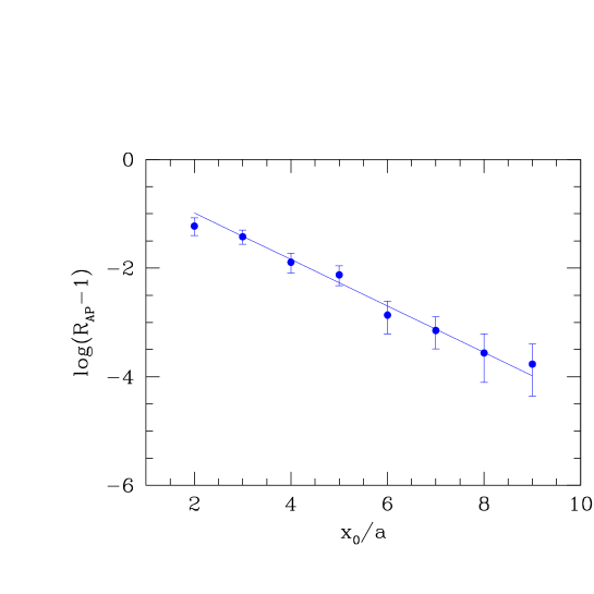
Figure 6: $R_{\rm AP}-1$ for $\kappa=0.1345$, $\beta=6.2$. The line represents a fit in the window $3a\leq x_{0}\leq 8a$.

By fitting $(R_{\rm AP}(x_{0})-1)$ to the above functional form in the appropriate range of $x_{0}$, one can extract the gap $\Delta$. A typical fit is shown in Fig. 6 from which we obtain the result quoted in the text,

$$r_{0}\Delta\approx 3.2\,.$$ (A.38)

It turns out that $\Delta$ depends very little on the bare quark mass, so that this result is used in the analysis of correlation functions in Section 3 at all values of the quark mass.

References

- [1] M. Lüscher, (1997), hep-ph/9711205.
- [2] R.D. Kenway, (1998), hep-lat/9810054.
- [3] CP-PACS Collaboration, R. Burkhalter et al., (1998), hep-lat/9810043.
- [4] M. Göckeler et al., Phys. Rev. D57 (1998) 5562 , hep-lat/9707021.
- [5] A. Cucchieri, M. Masetti, T. Mendes and R. Petronzio, Phys. Lett. B422 (1998) 212, hep-lat/9711040.
- [6] A. Cucchieri, T. Mendes and R. Petronzio, J. High Energy Phys. 05 (1998) 006, hep-lat/9804007.
- [7] R.G. Edwards, U.M. Heller and T.R. Klassen, Phys. Rev. Lett. 80 (1998) 3448, hep-lat/9711052.
- [8] D. Becirevic et al., (1998), hep-lat/9809129.
- [9] UKQCD Collaboration, K.C. Bowler et al., in preparation (1999).
- [10] ALPHA Collaboration, S. Capitani, M. Lüscher, R. Sommer and H. Wittig, (1998), hep-lat/9810063.
- [11] R. Gupta, (1997), hep-lat/9807028.
-
[12]
P. Bacilieri et al.,
Phys. Lett. B214 (1988) 115;
APE Collaboration, P. Bacilieri et al., Nucl. Phys. B317 (1989) 509. -
[13]
G. Kilcup,
Nucl. Phys. B (Proc. Suppl.) 9 (1988) 201;
R. Gupta, G. Guralnik, G.W. Kilcup and S.R. Sharpe, Phys. Rev. D43 (1991) 2003. - [14] T.A. DeGrand and R.D. Loft, Comput. Phys. Commun. 65 (1991) 84.
- [15] F. Butler, H. Chen, J. Sexton, A. Vaccarino and D. Weingarten, Nucl. Phys. Proc. Suppl. 26 (1992) 287.
- [16] T. DeGrand and M. Hecht, Phys. Lett. B275 (1992) 435.
- [17] A. Duncan et al., Phys. Rev. D51 (1995) 5101, hep-lat/9407025.
-
[18]
S. Güsken,
Nucl. Phys. B (Proc. Suppl.) 17 (1990) 361;
S. Güsken et al., Phys. Lett. B227 (1989) 266. - [19] C. Alexandrou, S. Güsken, F. Jegerlehner, K. Schilling and R. Sommer, Nucl. Phys. B414 (1994) 815, hep-lat/9211042.
- [20] UKQCD Collaboration, C.R. Allton et al., Phys. Rev. D47 (1993) 5128, hep-lat/9303009.
- [21] UKQCD Collaboration, P. Lacock, A. McKerrell, C. Michael, I.M. Stopher and P.W. Stephenson, Phys. Rev. D51 (1995) 6403, hep-lat/9412079.
- [22] C. Michael, Nucl. Phys. B259 (1985) 58.
- [23] M. Lüscher and U. Wolff, Nucl. Phys. B339 (1990) 222.
- [24] S. Sint, Nucl. Phys. B421 (1994) 135, hep-lat/9312079.
- [25] K. Jansen et al., Phys. Lett. B372 (1996) 275, hep-lat/9512009.
- [26] M. Lüscher, S. Sint, R. Sommer and P. Weisz, Nucl. Phys. B478 (1996) 365, hep-lat/9605038.
- [27] S. Sint and P. Weisz, Nucl. Phys. B502 (1997) 251, hep-lat/9704001.
- [28] M. Lüscher, R. Narayanan, P. Weisz and U. Wolff, Nucl. Phys. B384 (1992) 168, hep-lat/9207009.
- [29] M. Lüscher, Commun. Math. Phys. 54 (1977) 283.
- [30] M. Lüscher, S. Sint, R. Sommer, P. Weisz and U. Wolff, Nucl. Phys. B491 (1997) 323, hep-lat/9609035.
- [31] M. Lüscher, R. Sommer, P. Weisz and U. Wolff, Nucl. Phys. B413 (1994) 481, hep-lat/9309005.
- [32] M. Lüscher and P. Weisz, Nucl. Phys. B479 (1996) 429, hep-lat/9606016.
- [33] J. Heitger, (1999), hep-lat/9903016.
- [34] M. Guagnelli and R. Sommer, (1997), hep-lat/9709088.
- [35] R. Sommer, Nucl. Phys. B411 (1994) 839, hep-lat/9310022.
- [36] ALPHA Collaboration, M. Guagnelli, R. Sommer and H. Wittig, Nucl. Phys. B535 (1998) 389, hep-lat/9806005.
- [37] S. Fischer et al., Comp. Phys. Commun. 98 (1996) 20, hep-lat/9602019.
- [38] W. Bietenholz et al., (1998), hep-lat/9807013.
- [39] M.J. Teper, (1998), hep-th/9812187.
- [40] UKQCD Collaboration, C.R. Allton et al., Phys. Rev. D49 (1994) 474, hep-lat/9309002.