DESY 98-201
hep-lat/9903039

Confronting Instanton Perturbation Theory
with QCD Lattice Results

We exploit a recent lattice investigation (UKQCD) on the topological structure of the (quenched) QCD vacuum, in order to gain information on crucial building blocks of instanton perturbation theory. A central motivation is to further constrain our previous predictions of instanton-induced hard scattering processes. First, we address the generic problem of extracting quantitative information from cooled lattice data. We find a new scaling variable, interpreted as a “cooling radius”, which allows to combine lattice data for a whole range of lattice spacings and cooling sweeps. This variable strongly helps to extract information on the uncooled distributions of interest. After performing the continuum extrapolation of the instanton size and instanton-anti-instanton distance distributions, we find striking agreement with the theoretical predictions from instanton-perturbation theory, for instanton sizes $\mbox{\,\raisebox{1.29167pt}{$<$}$\!\!\!\!\!$\raisebox{-3.87495pt}{$\sim$}\,}0.5$ fm and distances $\mbox{\,\raisebox{1.29167pt}{$>$}$\!\!\!\!\!$\raisebox{-3.87495pt}{$\sim$}}\,0.5$ fm, respectively. These results imply first direct support for the validity of the known valley interaction between instantons and anti-instantons.

1. Non-abelian gauge theories like QCD are known to exhibit a rich vacuum structure. The latter includes topologically non-trivial fluctuations of the gauge fields, carrying an integer topological charge $Q$. The simplest building blocks of topological structure are instantons ($Q=+1$) and anti-instantons ($Q=-1$) which are well-known explicit solutions of the euclidean field equations in four dimensions [1].

Instantons are widely believed to play an important rôle in various long-distance aspects [2] of QCD:

First of all, they may provide a solution of the famous $U_{A}(1)$ problem [3] ($m_{\eta^{\prime}}\gg m_{\eta}$), with the corresponding pseudoscalar mass splitting related to the topological susceptibility in the pure gauge theory by the well-known Witten-Veneziano formula [4]. Moreover, a number of authors have attributed a strong connection of instantons with chiral symmetry breaking [5, 2] as well as the hadron and glueball spectrum.

However, there are also very important short-distance implications [?–?] of QCD instantons:

They are known to induce certain processes which violate chirality in accord with the general axial-anomaly relation [3] and which are forbidden in conventional perturbation theory. Of particular interest in this context is the deep-inelastic scattering (DIS) regime. Here, hard instanton-induced processes may both be calculated [?–?] within instanton-perturbation theory and possibly be detected experimentally [7, 11, 12, 13]. Since an experimental discovery of instanton-induced events would clearly be of basic significance, our ongoing theoretical and phenomenological study of the discovery potential of instanton-induced DIS events is well motivated.

On the other hand, there has been much recent activity in the lattice community to “measure” topological fluctuations in lattice simulations [14] of QCD. Being independent of perturbation theory, such simulations provide “snapshots” of the QCD vacuum including all possible non-perturbative features like instantons. They may be exploited to provide crucial support for important prerequisites of calculations in DIS, like the validity of instanton-perturbation theory and the dilute instanton-gas approximation for small instantons of size $\rho\leq{\mathcal{O}}(0.3)$ fm. Along these lines, we were able [9] to translate the lattice constraints into a “fiducial” kinematical region for our predictions of the instanton-induced DIS cross-section based on instanton-perturbation theory.

The purpose of the present letter is to present a more thorough confrontation of predictions from instanton-perturbation theory with recent lattice simulations. Specifically, we concentrate on recent high-statistics results from the UKQCD collaboration [15, 16], try to carefully discuss the effects of cooling and perform an extrapolation to the continuum before drawing our conclusions.

2. Let us start by considering various important quantities relevant for instanton ($I$)-induced scattering processes, that may both be calculated in $I$-perturbation theory and measured in lattice simulations. In $I$-perturbation theory one expands the path integral for the generating functional of the Green’s functions about the known, classical instanton solution $A_{\mu}=A^{(I)}_{\mu}+\ldots$ instead of the trivial vacuum $A^{(0)}_{\mu}=0$ (pQCD) and obtains a corresponding set of modified Feynman rules. Like in conventional pQCD, the strong gauge coupling $\alpha$ has to be small.

The $I$-induced contribution to hard scattering processes is typically encoded in the total cross-section [9, 10] associated with an $I$-induced partonic subprocess $q^{\prime}\,p\Rightarrow X$,

$$\sigma^{(I)}(q^{\prime}\,p\Rightarrow X) = \int d^{4}R\ \int\limits_{0}^{\infty}d\rho\int\limits_{0}^{\infty}d\overline{\rho}\ D(\rho)\,D(\overline{\rho})\int dU\,{\rm e}^{{-\frac{4\pi}{\alpha}}\,\Omega\left(U,\frac{R^{2}}{\rho\overline{\rho}},\frac{\overline{\rho}}{\rho}\right)}\,\{\ldots\}\,$$

$$\times F(\sqrt{-q^{\prime\,2}}\,\rho)\,F(\sqrt{-q^{\prime\,2}}\,\overline{\rho})F(\sqrt{-p^{2}}\,\rho)\,F(\sqrt{-p^{2}}\,\overline{\rho})\,{\rm e}^{{\rm i}\,(p+q^{\prime})\cdot R}\ .$$

$\sigma^{(I)}$ involves integrations over all $I\,[\overline{I}]$-“collective coordinates”, including the $I\,[\overline{I}]$-sizes $\rho\,[\overline{\rho}]$, the $I\overline{I}$-distance 4-vector $R_{\mu}$ and the $I\overline{I}$ relative colour orientation $U$. With each initial-state parton, there is an associated “form factor” [8, 9],

$$F(x)=x\,K_{1}(x)\ \left\{\begin{array}[]{lcllcll}&\sim&\sqrt{\pi/(2\,x)}\exp(-x)&{\rm\ for}&x&\rightarrow+\infty;\\[5.69054pt] &=&1&{\rm\ for}&x&=0;\\[5.69054pt] &&{\rm oscillating}&{\rm\ for}&x&{\rm\ imaginary}.\\ \end{array}\right.$$

An important quantity entering Eq. ( DESY 98-201 hep-lat/9903039 Confronting Instanton Perturbation Theory with QCD Lattice Results) as generic weight is the (reduced) $I$-size distribution in the dilute gas approximation, $D(\rho)$. It is known in the framework of $I$-perturbation theory for small $\alpha(\mu_{r})\ln(\rho\,\mu_{r})$, where $\mu_{r}$ is the renormalization scale. After its pioneering evaluation at 1-loop [3] for $N_{c}=2$ and its generalization [17] to arbitrary $N_{c}$, it is meanwhile available [18] in 2-loop renormalization-group (RG) invariant form, i.e. $D^{-1}\,dD/d\ln(\mu_{r})=\mathcal{O}(\alpha^{2})$,

$$D({\rho}) = \frac{d_{\overline{\rm MS}}}{\rho^{5}}\left(\frac{2\pi}{\alpha_{\overline{\rm MS}}(\mu_{r})}\right)^{2\,N_{c}}\exp{\left(-\frac{2\pi}{\alpha_{\overline{\rm MS}}(\mu_{r})}\right)}(\rho\,\mu_{r})^{\beta_{0}+(\beta_{1}-4\,N_{c}\beta_{0})\frac{\alpha_{\overline{\rm MS}}(\mu_{r})}{4\pi}},$$ (2)

$$d_{\overline{\rm MS}} = \frac{2\,{\rm e}^{5/6}}{\pi^{2}\,(N_{c}-1)!(N_{c}-2)!}\,{\rm e}^{-1.511374\,N_{c}+0.291746\,n_{f}}\ \ \mbox{(Ref.~{}\cite[cite]{[\@@bibref{}{dMS}{}{}]})};$$ (3)

$$\beta_{0} = \frac{11}{3}N_{c}-\frac{2}{3}n_{f};\hskip 28.45274pt\beta_{1}=\frac{34}{3}N_{c}^{2}-\left(\frac{13}{3}N_{c}-\frac{1}{N_{c}}\right)\,n_{f};\hskip 28.45274pt\gamma_{0}=3\frac{N_{c}^{2}-1}{N_{c}}.$$ (4)

For the case $n_{f}=0$, relevant for our comparison with lattice results below, the reduced size distribution $D(\rho)$, Eq. (2), equals the proper size distribution, i.e. the number of instantons per unit volume per unit size, $dn_{I}/d^{4}x\,d\rho$, (in the dilute gas approximation). On the other hand, for $n_{f}>0$, the proper size distribution reads

$$\frac{dn_{I}}{d^{4}x\,d\rho}\simeq\,D_{m}({\rho})=D({\rho})\,\prod_{i=1}^{n_{f}}(\rho\,m_{i}(\mu_{r}))\,(\rho\,\mu_{r})^{n_{f}\,\gamma_{0}\frac{\alpha_{\overline{\rm MS}}(\mu_{r})}{4\pi}},$$ (5)

for small $\rho\,m_{i}(\mu_{r})$, where $m_{i}(\mu_{r})$ are the running quark masses. However, even for $n_{f}>0$, only the reduced size distribution $D(\rho)$ appears in cross-sections like Eq. ( DESY 98-201 hep-lat/9903039 Confronting Instanton Perturbation Theory with QCD Lattice Results), since for small $m_{i}$, the mass-dependent factor in Eq. (5) is cancelled by corresponding terms from the external quarks.

The powerlaw behaviour of the (reduced) $I$-size distribution,

$$D({\rho})\sim\rho^{\beta_{0}-5+\mathcal{O}(\alpha)},$$ (6)

generically causes the dominant contributions to the $I$-size integrals to originate from the infrared (IR) regime (large $\rho$) and thus often spoils the applicability of $I$-perturbation theory. In deep-inelastic scattering, however, one parton $q^{\prime}$ say, carries a spacelike virtuality, such that the contribution of large instantons to the integrals ( DESY 98-201 hep-lat/9903039 Confronting Instanton Perturbation Theory with QCD Lattice Results) is exponentially suppressed (c. f. Eq. ( DESY 98-201 hep-lat/9903039 Confronting Instanton Perturbation Theory with QCD Lattice Results)),

$$F(\sqrt{-q^{\prime\,2}}\,\rho)\,F(\sqrt{-q^{\prime\,2}}\,\overline{\rho})\propto{\rm e}^{-Q^{\prime}\,(\rho+\overline{\rho})};\hskip 8.61108pt{\rm for\ }Q^{\prime}=\sqrt{-q^{\prime\,2}}>0,$$ (7)

and the predictivity of $I$-perturbation theory is retained for sufficiently large $Q^{\prime}$.

A second important ingredient into Eq. ( DESY 98-201 hep-lat/9903039 Confronting Instanton Perturbation Theory with QCD Lattice Results) is the function $\Omega(U,R^{2}/(\rho\overline{\rho}),\overline{\rho}/\rho)$, appearing in the exponent with a large numerical coefficient $4\pi/\alpha$. It incorporates the effects of final-state gluons. Within strict $I$-perturbation theory, it is given in form of a perturbative expansion [9, 20] for large $R^{2}$, while in the so-called $I\overline{I}$-valley approximation${}^{\ref{iai}}$ [21] $\Omega$ is associated with an analytically known closed expression [23] for the interaction between $I$ and $\bar{I}$, $\Omega=\alpha/(4\pi)S[A^{I\overline{I}}_{\mu}]-1$,

$$\Omega\left(U(v,z,\ldots),\frac{R^{2}}{\rho\overline{\rho}},\frac{\overline{\rho}}{\rho}\right)=\left(\frac{1}{2}-2\,z\right)\left(1+{v}^{2}\right)\Sigma_{{1}}+\left(\left(\frac{1}{2}-2\,z+4\,{z}^{2}\right)\left(1+{v}^{2}\right)^{2}+2\,{v}^{2}\right)\Sigma_{{2}}$$ (8)

with

$$\begin{array}[]{lclcl}\Sigma_{{1}}&=&-2\,{\frac{1-{\lambda}^{4}+4\,{\lambda}^{2}\ln(\lambda)}{\left({\lambda}^{2}-1\right)^{3}}};\hskip 38.74988pt\Sigma_{{2}}&=&{\frac{1-{\lambda}^{2}+\left(1+{\lambda}^{2}\right)\ln(\lambda)}{\left({\lambda}^{2}-1\right)^{3}}};\\[17.22217pt] \lambda&=&\frac{1}{2}\,\xi+\frac{1}{2}\,\sqrt{{\xi}^{2}-4};\hskip 38.74988pt\xi&=&\frac{R^{2}}{\rho\overline{\rho}}+\frac{\overline{\rho}}{\rho}+\frac{\rho}{\overline{\rho}}\,.\end{array}$$ (9)

The $I\overline{I}$-valley interaction (8) only depends on two of the four angle variables necessary in general to parametrize the relative color orientation $U$ (see e.g. Ref. [24]). In terms of these variabels ($v=\cos\alpha,\ z=\cos(\delta)^{2}$) and an additional azimuthal angle variable $\phi$, the integration over the $SU(3)$ group measure then takes the form [10]

$$\int dU=\frac{4}{\pi}\,\int_{-1}^{1}\!\mid v\mid\left(1-{v}^{4}\right){dv}\int_{0}^{\pi}d\phi\!\int_{0}^{\frac{1}{2}\,{\frac{1-2\,v\cos(\phi)+{v}^{2}}{1+{v}^{2}}}}\!\frac{dz}{1-2\,v\cos(\phi)+{v}^{2}}=1.$$ (10)

With these prerequisites in mind, let us next consider the group-averaged distribution of $I\overline{I}$ pairs, $dn_{I\overline{I}}/d^{4}x\,d^{4}R\,d\rho\,d\overline{\rho}$. This quantity is of basic interest for $I$-induced scattering processes ( DESY 98-201 hep-lat/9903039 Confronting Instanton Perturbation Theory with QCD Lattice Results), crucially depends on the $I\overline{I}$-interaction $\Omega$ and may be measured on the lattice. For the pure gauge theory ($n_{f}=0$) and in the dilute-gas approximation, it takes the form [9, 10]

$$\frac{dn_{I\overline{I}}}{d^{4}x\,d^{4}R\,d\rho\,d\overline{\rho}}\simeq D_{I\overline{I}}(R,\rho,\overline{\rho})=D(\rho)\,D(\overline{\rho})\ \int dU\,\exp\left[-\frac{4\pi}{\alpha_{\overline{\rm MS}}(s_{I\overline{I}}/\,\sqrt{\rho\overline{\rho}})}\,\Omega\left(U,\frac{R^{2}}{\rho\overline{\rho}},\frac{\overline{\rho}}{\rho}\right)\right],$$ (11)

with the scale factor $s_{I\overline{I}}=\mathcal{O}(1)$ parametrizing the residual scheme dependence.

In the deep-inelastic regime, relevant for instanton searches at HERA, the collective coordinate integrals involved in the hard cross-section ( DESY 98-201 hep-lat/9903039 Confronting Instanton Perturbation Theory with QCD Lattice Results) are known to be dominated by a unique saddle point [9]. Therefore, the Bjorken variables ($Q^{\prime},{x^{\prime}}$) of the $I$-induced subprocess in $e^{\pm}P$ scattering are effectively related in a one-to-one correspondence to the collective coordinates as (c. f. also Eqs. ( DESY 98-201 hep-lat/9903039 Confronting Instanton Perturbation Theory with QCD Lattice Results), (7)),

$$\rho\sim\overline{\rho}\sim 1/Q^{\prime}\ {\rm and}\ R^{2}\sim 1/(p+q^{\prime})^{2}\ \Rightarrow\ \rho\overline{\rho}/R^{2}\sim(p+q^{\prime})^{2}/Q^{\prime 2}=1/{x^{\prime}}-1.$$ (12)

Restrictions on the collective coordinates obtained from confronting predictions of $I$-perturbation theory with lattice results may thus be directly translated into a fiducial kinematical region for the predicted rate of $I$-induced processes at HERA [9]. This fact illustrates the great importance of lattice simulations for $I$-induced scattering processes and largely motivates the present analysis.

3. Before turning to our concrete analysis, we first have to address various topical problems associated with lattice data on instantons. The recent quenched QCD results ($n_{f}=0$) from the UKQCD collaboration [15, 16], which we shall use here, involve a lattice spacing $a=0.05-0.1$ fm and (roughly constant) volumes $V=l_{\rm space}^{\,3}\cdot l_{\rm time}$ of $32^{3}\,64\,a^{4}$ at $\beta(a)\equiv 6/g^{2}_{0}(a)=6.4$, $24^{3}\,48\,a^{4}$ at $\beta=6.2$ and $16^{3}\,48\,a^{4}$ at $\beta=6.0$.

In principle, such a lattice allows to study the properties of an ensemble of topological gauge field fluctuations ($I$’s and $\overline{I}$’s) with sizes $a<\rho<V^{1/4}$. However, in the raw data, ultraviolet fluctuations of wavelength $\mathcal{O}(a)$ dominate and completely mask the topological effects which are expected to be of much larger size. In order to make the latter visible, a certain “cooling” procedure has to be applied first. Cooling is a technique for removing the high-frequency non-topological excitations of the gauge-field, while affecting the topological fluctuations of much longer wavelength $\rho\gg a$ comparatively little. After cooling, $I$’s and $\overline{I}$’s can clearly be identified as bumps in the topological charge density and the Lagrange density. By applying sophisticated pattern-recognition algorithms, various distributions characterizing the ensemble of $I$’s and $\overline{I}$’s may be extracted.

However, during cooling instantons are also removed; either if they are very small (lattice artifacts) or through $I\bar{I}$ annihilation. In Ref. [15], so called under-relaxed (or slow) cooling is used to reduce the latter problem. Generically, the cooling procedure introduces substantial uncertainties in the extraction of physical information on the topological structure of the QCD vacuum. No objective criterium is yet available on the quantitative amount of “vacuum damage” introduced by it (see Refs. [14, 15]).

Since one is interested in the physics of the uncooled vacuum, it appears suggestive (at first) to try and extrapolate [14] the measured distributions to the limit of a vanishing number of cooling sweeps, $n_{\rm cool}\to 0$. However, to do so would be to ignore the fact that the pattern-recognition procedures become increasingly unreliable near that limit, since the extracted instanton density appears to strongly increase for decreasing $n_{\rm cool}$. Below a certain minimal number of cools, $(n_{\rm cool})_{\rm min}\,$, even the total topological charge $Q=n_{I}-n_{{\overline{I}}}$ starts to deviate from the plateau value it has for a whole range of larger $n_{\rm cool}$.

In view of these objections, we follow the alternative strategy of Ref. [15] to extract information about the physical vacuum. The method incorporates certain scaling studies that are important for the continuum limit $a\to 0$ and consists in the following steps: First, at $\beta=6.0$, say, one picks the smallest number of cooling sweeps for which the pattern-recognition starts to become reliable and the cooling history of the total topological charge enters a plateau. For straight cooling, one finds $(n_{\rm cool})_{\rm min}\simeq 10$ corresponding to $\simeq 23$ under-relaxed cools [16]. The next step is to search for further, so-called equivalent pairs $(\beta,n_{\rm cool})$, for which shape and normalization of specific distributions (expressed in physical units) essentially remain the same (see also Ref. [25]). The result of Ref. [15] were the pairs $(\beta,n_{\rm cool})=(6.0,23),\ (6.2,46),\ (6.4,80)$. With these equivalent, scaling data sets, the continuum limit is then performed with hopefully little “vacuum damage” due to cooling.

Yet, the crucial question remains at this point, whether the choice $(\beta,n_{\rm cool})=(6.0,23)$ as a “starting pair” for the equivalent data is somehow distinguished, i. e. physically meaningful. In this context, let us present an intriguing line of arguments:

“Equivalent” data should first of all be characterized by a similar amount of cooling. For $n_{\rm cool}$ cooling sweeps, an effective “cooling radius” $r_{\rm cool}$ in physical units${}^{\ref{sommer}}$ may be defined, via a (qualitative) random walk argument, as

$$\frac{r_{\rm cool}}{2\,r_{0}}={\rm const}\,(\sqrt{n_{\rm cool}})^{1+\delta}\,\frac{a}{2\,r_{0}};\hskip 25.83325pt\delta{\rm\ small}.$$ (13)

The three equivalent pairs $(\beta,n_{\rm cool})$ above, indeed, turn out to have a very similar value of $r_{\rm cool}$ (see Table 1).

($\beta,n_{\rm cool}$)	($6.0,23$)	($6.2,46$)	($6.4,80$)
$\sqrt{n_{\rm cool}}\,\frac{a}{2r_{0}}$	0.447(2)	0.460(2)	0.459(2)

Table 1: The “cooling radius” for the equivalent data sets is similar.

Amazingly, the usefulness of the variable (13) seems to be much greater. In Fig. 1, we illustrate that the average instanton size $\langle\rho\rangle$ in physical units from Ref. [15], for all available values of ($\beta,n_{\rm cool}$), fits onto a single

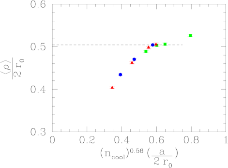
Figure 1: The average instanton size from Ref. [15] in physical units for $\beta=6.0\,[\Box]$, $6.2\,[\circ]$, $6.4\,[\triangle]$ and for all available values of $n_{\rm cool}$ as a function of the effective cooling radius (13). There is a clear indication of a plateau corresponding to $\langle\rho\rangle\simeq 0.5$ fm, which is interpreted in the text. The quantity $r_{0}$ denotes the Sommer scale${}^{\ref{sommer}}$ with $2\,r_{0}\simeq 1$ fm.

smooth curve as function of $r_{\rm cool}$ in Eq. (13) with $\delta$ small. In contrast, one obtains three widely spaced curves, if $\langle\rho\rangle/2r_{0}$ is displayed as a function of $n_{\rm cool}$ alone for fixed $\beta=6.0,\,6.2$ and $6.4$, respectively. The same scaling with $r_{\rm cool}$ holds practically for all quantities extracted in Ref. [15], characterizing the instanton ensemble on the lattice.

Perhaps the most striking feature of Fig. 1 is the clear indication of a plateau corresponding to $\langle\rho\rangle\simeq 0.5$ fm. Let us try to provide some interpretation for it. Suppose, the localized fluctuations on the lattice are a mixture of two distinct ensembles, separated by a certain gap in their respective average sizes. For example, one expects fluctuations that are lattice artifacts typically located around smaller sizes $\mathcal{O}({\rm few}\cdot a)$, while the physical instanton sizes are peaking around $\rho\simeq r_{0}\simeq 0.5$ fm. By gradually increasing the cooling radius $r_{\rm cool}$, we first filter out the smaller artifacts, leading clearly to a corresponding increase in the effective $\langle\rho\rangle$. When the radius of our filter further increases, one then expects a plateau in $\langle\rho\rangle$ to indicate that the small artifacts have been mostly wiped out, while the much larger physical instantons are not yet strongly affected. Eventually, the instantons will also start to be erased, leading again to an increase in $\langle\rho\rangle$.

In conclusion, we think that the plateau region is the correct regime for extracting physical information about instantons. The equivalent data sets of Ref. [15] are precisely located around the plateau.

Our scaling variable $r_{\rm cool}$ allows to combine lattice data for a whole range of lattice spacings $a$ and cools $n_{\rm cool}$, which strongly helps to increase the separation power between the $a$-dependent artifacts and the instantons of a certain physical size. In future analyses, it may be worthwhile to determine the unknown constant in the definition (13) of $r_{\rm cool}$, e. g. by means of calibration via cooling an isolated instanton until it disappears.

4. We are now ready to discuss the continuum limit of the UKQCD data for the size distribution of $I$’s and ${\overline{I}}$’s, $dn_{I+{\overline{I}}}/d^{4}x\,d\rho$, and to compare it with the dilute-gas prediction $D_{I+{\overline{I}}}(\rho)=2\,D(\rho)$ of $I$-perturbation theory, Eq. (2), for $n_{f}=0$.

We note, first of all, that the (small) residual $a$ dependence of the equivalent data for the size distribution in physical units may be parametrized as

$$(2\,r_{0})^{5}\,\frac{dn_{I+{\overline{I}}}}{d^{4}x\,d\rho}=\mbox{\ function}\,\left(\frac{\rho}{\langle\rho(a)\rangle}\right).$$ (14)

The continuum limit of Eq. (14) can thus be performed quite reliably, by simply rescaling the arguments $\rho\to\langle\rho(0)\rangle/\langle\rho(a)\rangle\cdot\rho$. Here, $\langle\rho(0)\rangle/2r_{0}=0.518(5)$ denotes the continuum limit of the weakly varying average $\rho$ values, $\langle\rho(a)\rangle$. As in Ref. [15], $\langle\rho(a)\rangle/2r_{0}$ was extrapolated linearly in $(a/r_{0})^{2}$. The resulting continuum size distribution obtained by the above rescaling from the three equivalent data sets is displayed in Fig. 2. It scales nicely.

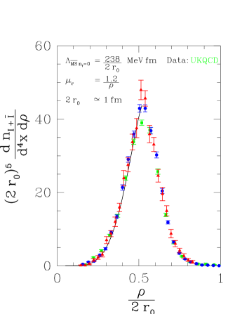
Figure 2: Continuum limit of “equivalent” UKQCD data [15] for the ($I+\overline{I}$)-size distribution at $(\beta,n_{\rm cools})=(6.0,23)\,[\Box],\ (6.2,46)\,[\circ],\ (6.4,80)\,[\triangle]$. The striking agreement with $2\,D(\rho)$ of $I$-perturbation theory from (2) is apparent. The 3-loop form of $\alpha_{\overline{\rm MS}}$ with $\Lambda_{\overline{\rm MS}\,n_{f}=0}$ from ALPHA [28] was used. (a) Log-log plot to exhibit the expected power law $\sim\rho^{6}$ and the agreement in magnitude for small $\rho$ over a wide range of $\mu_{r}$. The dashed error band results from varying $\Lambda_{\overline{\rm MS}\,n_{f}=0}$ and $\mu_{r}$ within its error and given range, respectively; (b) For $\mu_{r}=1.2/\rho$, the agreement extends up to the peak.

We are now ready to perform a quantitative comparison with $I$-perturbation theory. The corresponding prediction (2) is a power law for small $\rho$, i. e. approximately $D\sim\rho^{6}$ for $n_{f}=0$. Due to its 2-loop RG-invariance the normalization of $D_{I+\overline{I}}(\rho)$ is practically independent of the renormalization scale $\mu_{r}$ over a wide range. It is strongly dependent on $r_{0}\,\Lambda_{\overline{\rm MS}}$, for which we take the most recent, accurate lattice result by the ALPHA collaboration [28], $2\,r_{0}\,\Lambda_{\overline{\rm MS}\,n_{f}=0}=(238\pm 19)$ MeV fm. In Fig. 2 (a) we display both this parameter-free prediction (2) of $I$-perturbation theory and the continuum limit of the UKQCD data in a log-log plot, to clearly exhibit the expected power law in $\rho$. The agreement in shape and normalization for $\rho/2r_{0}\mbox{\,\raisebox{1.29167pt}{$<$}$\!\!\!\!\!$\raisebox{-3.87495pt}{$\sim$}\,}0.3$ is striking, indeed, notably in view of the often criticized cooling procedure and the strong sensitivity to $\Lambda_{\overline{\rm MS}}$. One may argue that a choice $\rho\mu_{r}=\mathcal{O}(1)$ is theoretically favoured, since it tends to suppress $\ln(\rho\mu_{r})$ corrections. Indeed, as apparent from Fig. 2 (b), the agreement extends in this case up to the peak around $\rho/2r_{0}\simeq 0.5$.

At this point, an interesting way to proceed is to define a non-perturbative “instanton-scheme” for $\alpha$ by the requirement that the theoretical expression (2) for the size distribution $D_{I+\overline{I}}(\rho)$ precisely reproduces the corresponding lattice data,

$$\rho^{5}\,\frac{dn_{I+{\overline{I}}}}{d^{4}x\,d\rho}\equiv 2\,d_{\overline{\rm MS}}\left(\frac{2\pi}{\alpha_{\rm I}(\frac{1}{\rho})}\right)^{2\,N_{c}}\exp{\left(-\frac{2\pi}{\alpha_{\rm I}(\frac{1}{\rho})}\right)}s_{\rm I}^{\beta_{0}+\frac{\alpha_{\rm I}(\frac{1}{\rho})}{4\pi}(\beta_{1}-4\,N_{c}\beta_{0})}.$$ (15)

By comparing in the perturbative regime with the $\overline{\rm MS}$ form (2) for $\mu_{r}=s/\rho$, we arrive at a standard scheme conversion formula,

$$\alpha_{\overline{\rm MS}}(s/\rho)=\alpha_{\rm I}(1/\rho)-\frac{\beta_{0}}{2\pi}\ln(s/s_{\rm I})\,\alpha_{\rm I}(1/\rho)^{2}+\mathcal{O}(\alpha_{\rm I}(1/\rho)^{3}),$$ (16)

with

$$s_{\rm I}=\frac{\Lambda_{\overline{\rm MS}}}{\Lambda_{\rm I}}\hskip 28.45274pt\mbox{\ and\ }\hskip 28.45274pt\alpha_{\overline{\rm MS}}(s_{\rm I}/\rho)\simeq\alpha_{\rm I}(1/\rho).$$ (17)

Next, we note that as a function of $\alpha_{\rm I}$, $D_{I+\overline{I}}(\rho)$ has a peak structure like the lattice data, with maximum at

$$\alpha_{\rm I\,\mid max}=\frac{\pi}{N_{c}}\,\frac{2}{1+\sqrt{1+\frac{1}{N_{c}}\ln(s_{\rm I})(2\beta_{0}-\frac{\beta_{1}}{2N_{c}})}}.$$ (18)

The scale factor $s_{\rm I}$ of the $I$-scheme is non-perturbatively and uniquely determined by the peak value of the lattice data for the size distribution. Using the very good Gaussian fit to all data in Fig. 2 (b),

$$(2\,r_{0})^{5}\,\frac{dn_{I+{\overline{I}}}}{d^{4}x\,d\rho}_{\mid{\rm fit}}=\frac{(a\rho)^{6}\exp\left(-(c\rho)^{2}\right)}{(1+(b\rho)^{p})};\hskip 25.83325pt\left\{\begin{array}[]{lcl}a&=&4.908(40)/2r_{0}\\ b&=&1.683(15)/2r_{0}\\ c&=&2.525(52)/2r_{0}\\ p&=&12.43(25)\end{array}\right.$$ (19)

we find

$$s_{\rm I}=1.18\mbox{\ and\ }\alpha_{\rm I\,\mid max}=0.98.$$ (20)

In the perturbative regime, the $I$-scheme is thus quite close to the $\overline{\rm MS}$-scheme (c. f. Eq. (17)).

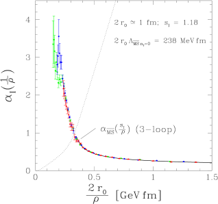
Figure 3: (a) Running coupling $\alpha_{\rm I}$ in the “instanton” scheme, extracted via Eq. (15) from the $I+{\overline{I}}$ size distribution. The same UKQCD data as in Fig. 2 have been used. The dotted line denotes a possible second solution vanishing in the IR limit. The excellent agreement with the corresponding 3-loop perturbative $\alpha_{\overline{\rm MS}}(s_{\rm I}/\rho)\simeq\alpha_{\rm I}(1/\rho)$ down to $1/\rho\simeq 0.4$ GeV is apparent (solid line). (b) At large distances, $\alpha_{\rm I}$ from (a) appears to be quite close to $\alpha_{\rm q\overline{q}}$ defined via the static $q\overline{q}$ potential, with $(4/3r^{2})\,\alpha_{\rm q\overline{q}}(1/r)$ approaching the string tension $\sigma$ for large $r$ and [27] $2\,r_{0}\,\sqrt{\sigma}=(472.4\pm 4.3)$ MeV fm.

We are now able to extract for each data point of the $I+{\overline{I}}$ size distribution a corresponding value of $\alpha_{\rm I}$, as illustrated in Fig. 3. Actually, besides the asymptotically free solution [$\alpha_{\rm I}$] to Eq. (15), there is a second one [$\alpha^{(2)}_{\rm I}$] (dotted line in Fig. 3), with a monopole-like relation to $\alpha_{\rm I}$,

$$\alpha^{(2)}_{\rm I}\cdot\alpha_{\rm I}=\mathcal{O}(1),$$ (21)

vanishing in the IR-limit and increasing like $\alpha^{(2)}_{I}(\mu)\propto(\mu/\Lambda)^{\beta 0/2N_{c}}$ in the UV-limit. This observation may be of interest in the context of Ref. [29].

It is remarkable that in the non-perturbative long-distance regime, $\rho/2r_{0}\mbox{\,\raisebox{1.29167pt}{$>$}$\!\!\!\!\!$\raisebox{-3.87495pt}{$\sim$}}\,0.5$, $\alpha_{\rm I}(1/\rho)$ from the $I+{\overline{I}}$ size distribution tends to approach $\alpha_{\rm q\overline{q}}(1/\rho)$ defined via the static $q\overline{q}$ potential, $V_{\rm q\overline{q}}$,

$$\frac{4}{3}\frac{\alpha_{\rm q\overline{q}}(1/r)}{r^{2}}\equiv\frac{dV_{\rm q\overline{q}}(r)}{dr}\simeq\ \sigma+\frac{\pi}{12}\frac{1}{r^{2}}\stackrel{{\scriptstyle r\rightarrow\infty}}{{\Rightarrow}}\sigma,$$ (22)

with string tension $\sigma$. This is illustrated in Fig. 3 (b).

In summary, $\alpha_{\rm I}$ as non-perturbatively defined through Eq. (15), is close to the $\overline{\rm MS}$-scheme in the perturbative short-distance region and to the $q\overline{q}$-scheme in the non-perturbative long-distance regime. Figs. 2 (b) and 3 (b) illustrate that the transition between perturbative and confinement-sensitive physics seems to be rather sharp and located where the instanton density peaks, around $\rho\simeq 0.5$ fm.

The above results also suggest the following working hypothesis [30], which might considerably enlarge the region of applicability of predictions like ( DESY 98-201 hep-lat/9903039 Confronting Instanton Perturbation Theory with QCD Lattice Results) and (11) for observables associated with sufficiently dilute instantons. Whenever one encounters the $I$-size distribution $D(\rho)$ within the perturbative calculus, one may try to replace the indefinitely growing perturbative expression $D(\rho)\sim\rho^{\beta_{0}-5}$ for the $I$-size distribution by the functional form actually extracted from the lattice (see e.g. Eq. (19)). Obviously, such an attempt eliminitates the problematic IR divergencies of $I$-size integrals. Due to the strong peaking of the measured size distribution (19), only $I$’s of size $\rho\simeq 0.5$ fm effectively contribute to the observables of interest and the dilute gas approximation may well continue to hold qualitatively up to the peak around $0.5$ fm.

5. As an immediate first application of this strategy, let us turn to the group-averaged distribution of $I\overline{I}$-pairs, $D_{I\overline{I}}(R,\rho,\overline{\rho})$, in the dilute gas approximation, Eq. (11). While the conservative prediction of instanton perturbation theory is restricted to $\rho,\overline{\rho}\mbox{\,\raisebox{1.29167pt}{$<$}$\!\!\!\!\!$\raisebox{-3.87495pt}{$\sim$}\,}0.3-0.5$ fm, UKQCD lattice results [15, 16] are available up to now only for the $I\overline{I}$-distance distribution, integrated over all values of $\rho,\overline{\rho}$,

$$\frac{dn_{I\overline{I}}}{d^{4}x\,d^{4}R}=\int\,\int d\rho\,d\overline{\rho}\,\frac{dn_{I\overline{I}}}{d^{4}x\,d^{4}R\,d\rho\,d\overline{\rho}}\,.$$ (23)

This is the point to exploit the above working hypothesis: We now replace in the theoretical expression for the $I\overline{I}$-distance distribution (23) along with Eq. (11) the perturbative form for $D(\rho)$ by the Gaussian fit (19) to the UKQCD lattice data. We are left with only one free parameter, the scale factor $s_{I\overline{I}}=\mathcal{O}(1)$ in the running coupling $\alpha_{\overline{\rm MS}}(s_{I\overline{I}}/\sqrt{\rho\overline{\rho}})$. On account of the peaking of the size distributions in Eq. (11), the running coupling at a momentum scale around $\mathcal{O}(0.3)$ GeV enters significantly. In this region, we make use of the non-perturbatively extracted coupling in the $I$-scheme (Fig. 3), with

$$\alpha_{\overline{\rm MS}}\left(\frac{s_{I\overline{I}}}{\sqrt{\rho\overline{\rho}}}\right)\Rightarrow\alpha_{I}\left(\frac{s_{I\overline{I}}}{s_{I}}\frac{1}{\sqrt{\rho\overline{\rho}}}\right);\hskip 25.83325pts_{I}=1.18,$$ (24)

as a smooth continuation of the perturbative $\overline{\rm MS}$ coupling (c. f. Eq. (17)). In the quantitative evaluation of Eqs. (23) and (11), we perform two integrals of the group integration and the two integrals over the $I$- and ${\overline{I}}$-sizes numerically.

Before being able to compare this theoretical prediction of the $I\overline{I}$-distance distribution with lattice results, we have to perform the continuum limit of the respective UKQCD data [16]. This we do in complete analogy to the method described in Sect. 4., Eq. (14), for the $I$-size distribution. Unfortunately, the equivalent data for $\beta=6.4$ are missing in this case [16]. The equivalent data for the remaining two $\beta$ values, $(\beta,n_{\rm cool})=(6.0,23)$ and $(6.2,46)$, again are well compatible with a scaling law, like Eq. (14),

$$\frac{dn_{I\overline{I}}}{d^{4}x\,d^{4}R}\,\Bigg{/}\frac{dn_{I\overline{I}}}{d^{4}x\,d^{4}R}_{\mid\,R\ {\rm large}}=\ {\rm function}\left(\frac{R}{r(a)}\right).$$ (25)

By extrapolating the scaling factor $\lambda(a)\equiv r(a)/r_{\mid\,\beta=6.2}$ linearly in $(a/r_{0})^{2}$, we find from requiring best overall scaling (25) of the two equivalent data sets, $\lambda_{I\overline{I}}(a)=1.32-69.75(a/2r_{0})^{2}$. The resulting “continuum data” obtained from the simple rescaling of the arguments, $R\to r(0)/r(a)\,R=\lambda(0)/\lambda(a)\,R$, are displayed in Fig. 4 and exhibit good scaling.

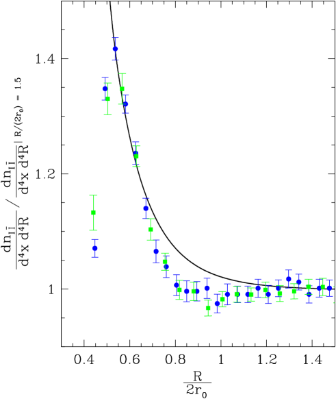
Figure 4: Continuum limit of “equivalent” UKQCD data [16] for the $I\overline{I}$-distance distribution, $dn_{I\overline{I}}/d^{4}x\,d^{4}R$, normalized to its value at $R/2r_{0}=1.5$, at $(\beta,n_{\rm cools})=(6.0,23)\,[\Box],\ (6.2,46)\,[\circ]$. As discussed in the text, the solid line denotes the theoretical prediction from instanton-perturbation theory based on the valley form of the $I\overline{I}$-interaction.

The solid line in Fig. 4 denotes the theoretical prediction discussed above with the scale factor $s_{I\overline{I}}=0.82$ being $\mathcal{O}(1)$ as expected.

We note a very good agreement with the lattice data down to $I\overline{I}$-distances $R/\langle\rho\rangle\simeq 1$, corresponding to $\xi\mbox{\,\raisebox{1.29167pt}{$>$}$\!\!\!\!\!$\raisebox{-3.87495pt}{$\sim$}}\,3$ (c. f. Eq. (9)). These results imply first direct support for the validity of the valley interaction (8) between instantons and anti-instantons.

References

- [1] A. Belavin, A. Polyakov, A. Schwarz and Yu. Tyupkin, Phys. Lett. B 59 (1975) 85.
- [2] T. Schäfer and E.V. Shuryak, Rev. Mod. Phys. 70 (1998) 323.
- [3] G. ‘t Hooft, Phys. Rev. Lett. 37 (1976) 8; Phys. Rev. D 14 (1976) 3432; Phys. Rev. D 18 (1978) 2199 (Erratum).
- [4] E. Witten, Nucl. Phys. B 156 (1979) 269; G. Veneziano, Nucl. Phys. B 159 (1979) 213.
- [5] D. Diakonov, hep-ph/9602375, Lectures at the 1995 Enrico Fermi School.
- [6] I. Balitsky and V. Braun, Phys. Lett. B 314 (1993) 237.
- [7] A. Ringwald and F. Schrempp, hep-ph/9411217, in: Quarks ‘94, Proc. 8th Int. Seminar, Vladimir, Russia, 1994, pp. 170-193.
- [8] S. Moch, A. Ringwald and F. Schrempp, Nucl. Phys. B 507 (1997) 134.
- [9] A. Ringwald and F. Schrempp, hep-ph/9806528, Phys. Lett. B 438 (1998) 217.
- [10] S. Moch, A. Ringwald and F. Schrempp, to be published.
- [11] M. Gibbs, A. Ringwald and F. Schrempp, hep-ph/9506392, in: Proc. Workshop on Deep Inelastic Scattering and QCD, Paris, 1995, pp. 341-344.
- [12] A. Ringwald and F. Schrempp, hep-ph/9610213, in: Quarks ‘96, Proc. 9th Int. Seminar, Yaroslavl, Russia, 1996, pp. 29-54.
- [13] A. Ringwald and F. Schrempp, DESY 97-115, hep-ph/9706399, in: Proc. 5th International Workshop on Deep Inelastic Scattering and QCD (DIS 97), Chicago, 1997, pp. 781-786.
- [14] see e. g.: J. Negele, hep-lat/9810053, Review at Lattice ‘98, and references cited therein.
- [15] D.A. Smith and M.J. Teper, (UKQCD Collab.), hep-lat/9801008, Phys. Rev. D 58 (1998) 014505.
- [16] M. Teper, private communication.
- [17] C. Bernard, Phys. Rev. D 19 (1979) 3013.
- [18] T. Morris, D. Ross and C. Sachrajda, Nucl. Phys. B 255 (1985) 115.
- [19] A. Hasenfratz and P. Hasenfratz, Nucl. Phys. B 193 (1981) 210; M. Lüscher, Nucl. Phys. B 205 (1982) 483; G. ‘t Hooft, Phys. Rep. 142 (1986) 357.
- [20] P. Arnold and M. Mattis, Phys. Rev. D 44 (1991) 3650; A. Mueller, Nucl. Phys. B 364 (1991) 109; D. Diakonov and V. Petrov, in: Proc. of the 26th LNPI Winter School, (Leningrad, 1991), pp. 8-64.
- [21] A. Yung, Nucl. Phys. B 297 (1988) 47.
- [22] V.V. Khoze and A. Ringwald, Phys. Lett. B 259 (1991) 106.
- [23] J. Verbaarschot, Nucl. Phys. B 362 (1991) 33.
- [24] I. Balitsky and V. Braun, Phys. Rev. D 47 (1993) 1879.
- [25] U. Sharan and M. Teper, (UKQCD Collab.), hep-lat/9812009.
- [26] R. Sommer, hep-lat/9310022, Nucl. Phys. B 411 (1994) 839.
- [27] M. Guagnelli, R. Sommer and H. Wittig, hep-lat/9806005, Nucl. Phys. B 535 (1998) 389.
- [28] S. Capitani, M. Lüscher, R. Sommer and H. Wittig, (ALPHA Collab.), hep-lat/9810063.
- [29] I. Kogan and M. Shifman, hep-th/9504141, Phys. Rev. Lett. 75 (1995) 2085.
- [30] A. Ringwald and F. Schrempp, hep-ph/9812359, in: Proc. 3rd UK Phenomenology Workshop on HERA Physics, to appear in Journal of Physics G.