Inverse Symmetry Breaking on the lattice: an accurate MC study

Abstract

We present here a new MC study of ISB at finite temperature in a $Z_{2}\times Z_{2}$ $\lambda\phi^{4}$ model in four dimensions. The results of our simulations, even if not conclusive, are favourable to ISB. Detection of the effect required measuring some critical couplings with six-digits precision, a level of accuracy that could be achieved only by a careful use of FSS techniques. The gap equations for the Debye masses, resulting from the resummation of the ring diagrams, seem to provide a qualitatively correct description of the data, while the simple one-loop formulae appear to be inadequate.

PACS: 05.70.Jk, 11.10.Wx, 98.80.Cq

Keywords: Finite temperature, Phase transitions, Inverse symmetry breaking, Symmetry non-restoration.

DFTUZ preprint 98/27     Napoli preprint 7/99     hep-lat/9903027

1 Introduction

In 1974, in his classic paper on thermal field theory, Steven Weinberg, quoting S. Coleman, reported on the unusual behavior of certain particle theory models at high temperatures. Using the example of a simple $O(N_{1})\times O(N_{2})$ scalar $\phi^{4}$ model, he showed that it is possible to induce spontaneous symmetry breaking at arbitrarily high temperatures. He named this funny phenomenon Inverse Symmetry Breaking (ISB) or Symmetry-Non-Restoration (SNR), depending on whether the ground state was disordered or ordered at zero temperature. In order to make this seemingly paradoxical statement easier to accept, he observed that in Nature there is a substance, the Rochelle salt, that does exhibit this sort of inverse behavior. Its crystals are orthorhombic below the lower Curie point (-$18^{~{}0}C$), and monoclinic above it, which means that the crystal has a $\it larger$ symmetry group at the $\it lower$ temperature! Of course, Weinberg’s statement was much stronger than this example, for he claimed that order could persist for ever, no matter how high the temperature, while the Rochelle salt, if heated enough, eventually melts.

In any case, ISB and SNR would have probably remained relegated among the amenities of field theory, if it were not for the fact that this mechanism can be implemented in realistic particle models and then applied to important cosmological issues related to the thermal history of the Early Universe. This is not the right place to discuss these very interesting applications of ISB and SNR, but to give the reader an idea of the number and relevance of the issues that have been treated , we just make a list and quote some references. Following the historical order, ISB and SNR were applied to: the breaking of CP symmetry [2], the monopole problem [3], baryogenesis [4], inflation [5], the breaking of P, strong CP and Peccei-Quinn symmetries [6] and finally supersymmetry [7].

The potential importance of ISB and SNR for cosmology induced several authors to study these phenomena more accurately, than was done in Weinberg’s original paper. His analysis relied, in fact, on a simple one-loop computation, and so it was natural to question if higher order corrections would have changed the scenario. This was not an idle question for at least two reasons. On one side, it is well known that at high temperature the reliability of perturbation theory is questionable, because powers of the temperature can compensate for powers of the coupling constants, spoiling the expansion. On the other side, and maybe more importantly, when one tries to induce ISB or SNR in realistic particle models, one is generally forced to consider rather large couplings in the scalar sector, in order to overcome the action of the gauge fields, which always work in favour of symmetry restoration at high temperature, and thus it becomes important to explore the robustness of ISB and SNR with respect to the coupling strengths.

The problem was attacked using a variety of approaches: large $N$ expansions [8], the Gaussian effective potential [9], the constraint effective potential [10], gap equations [11], the average effective action [12] and recently chiral effective Lagrangians [13]. The results were contradictory: some authors concluded that ISB and SNR are artifacts of the one-loop approximation, while others confirmed the existence of these phenomena, but observed that higher order-corrections have the effect of reducing the size of the parameter region for which they can occur.

This state of things motivated us to start a program of MC simulations to study ISB, which seemed to us the only way to carry a fully non-perturbative analysis of this problem. We chose the simplest model that can exhibit ISB, namely a $Z_{2}\times Z_{2}$ two-scalars $\phi^{4}_{d}$ theory. In the first run, we simulated the model in three dimensions [14] and afterwards we followed with four [15]. In both cases we found no sign of ISB, despite the fact that, for the values of the coupling constants that were simulated, the one-loop conditions for ISB were strongly satisfied. Recently, the authors of ref.[16] examined a $Z_{2}\times O(4)$ two-scalar $\phi^{4}$ model, in four dimensions, and claimed to have found a clear evidence that ISB was taking place.

In this paper we present the results of a new series of simulations of our $Z_{2}\times Z_{2}$ model. The strategy that we have followed is essentially the same of our previous paper [15]. Our two scalar model depends on five parameters, three coupling constants $\lambda_{1},\lambda_{2}$ and $\lambda$, and two hopping parameters $\kappa_{1}$ and $\kappa_{2}$. We fixed once and for all the values of the coupling constants: with respect to [15], this time we enforced the perturbative conditions for ISB (in the direction of the field $\phi_{2}$) much more strongly and at the same time we took smaller values in order to be closer to the perturbative region. We then studied the phase diagram as a function of the two hopping parameters. In the $(\kappa_{1},\kappa_{2})$ plane we found transition lines of first and second order, but since we were interested in ISB, we focused our efforts on the critical line for the breaking of the field $\phi_{2}$. This line is roughly parallel to the $\kappa_{1}$ axis and the aim was to determine in what direction it shifts, when the temperature is increased: ISB requires that, for $T>0$, it shifts towards smaller values of $\kappa_{2}$, at least in a neighbourhood of the scaling region.

As it is well known, finite temperatures are simulated by lattices with a finite extension $N_{t}$ in one direction, the temperature being $T=1/(N_{t}a)$, with $a$ the lattice spacing. What made the simulations very hard is the extreme smallness of the effect that we show in this paper: even at the highest temperature, which corresponds to $N_{t}=2$, in order to detect the shift reliably, it was necessary to measure the critical values of $\kappa_{2}$, both for $T=0$ and for $T>0$, with six significant digits! As it is well known, the only safe way to achieve such a huge precision is via an accurate analysis of Finite Size Scaling (FSS). This required large lattices and tremendous statistics: in one case, for example, we simulated a $20^{4}$ lattice, with $8\times 10^{6}$ iterations.

For $N_{t}=2$, the direction of the shift was favourable to ISB, but we cannot consider this result as conclusive. Due to the difficulty of the measurements, we could not simulate larger values of $N_{t}$, as it is necessary in order to make sure, via scaling analysis, that things would go in the same way for all $N_{t}$’s.

As a check, we compared the theoretical predictions with the MC value of the critical temperature for which we observed ISB. While the simple one-loop estimate is grossly incorrect, we found a reasonable agreement with the value obtained from the gap equations, which result from resumming the ring diagrams of the perturbative series [17]. These equations seem to give a qualitatively correct description of the MC data, and explain as well why we did not find ISB in our previous simulations in [15].

We close this introductory Section with a plan of the paper: in Section 2 we introduce our lattice model and discuss its phase diagram at $T=0$. In Section 3 we review the perturbative picture of ISB, while in Section 4 we discuss in detail our strategy to study ISB on the lattice. In Section 5 we discuss how the results of the simulations compare with the theoretical predictions, while Section 6 contains a discussion of the recent MC studies in [15] and [16]. Finally, Section 7 contains our concluding remarks.

2 The model and its lattice formulation

We consider the theory for two real scalar fields in $4$ euclidean dimensions, described by the bare (euclidean) action:

$$S=\int d^{4}x\Big{\{}\sum_{i=1,2}\Big{[}\frac{1}{2}(\partial_{\mu}\Phi_{i}^{(0)2})+\frac{1}{2}\overline{m}_{i}^{(0)2}\Phi_{i}^{(0)2}+\frac{g_{i}^{(0)}}{4!}\Phi_{i}^{(0)4}\Big{]}+\frac{1}{4}g^{(0)}\Phi_{1}^{(0)2}\Phi_{2}^{(0)2}\Big{\}}.$$ (1)

What will be essential for ISB and SNR, in the above action the quartic bare coupling $g^{(0)}$ can be negative. If $g^{(0)}>0$ the condition of boundedness from below of the potential is satisfied if:

$$g_{1}^{(0)}>0,~{}~{}~{}g_{2}^{(0)}>0,$$

$$g_{1}^{(0)}\;g_{2}^{(0)}>9\;g^{(0)2}.$$ (2)

When regularized on an infinite four-dimensional cubic lattice of points $\Omega$ with lattice spacing $a$, the above action is replaced by its discretized version

$$S_{L} = \sum_{x\in\Omega}a^{4}\Big{\{}\sum_{i=1,2}\Big{[}\sum_{\mu}\frac{1}{2}(\Delta^{(a)}_{\mu}\Phi_{i,L})^{2}(x)+\frac{1}{2}\overline{m}_{i}^{(0)2}\Phi_{i,L}^{2}(x)+\frac{g_{i}^{(0)}}{4!}\Phi^{4}_{i,L}(x)\Big{]}+$$ (3)

$$\;\;\;\;\;\;\;\;\;\;\;\;+\frac{g^{(0)}}{4}\;\Phi_{1,L}^{2}(x)\Phi_{2,L}^{2}(x)\Big{\}},$$

where $\Delta^{(a)}_{\mu}$ is the lattice derivative operator in the direction $\mu$:

$$\Delta^{(a)}_{\mu}\Phi_{i,L}(x)\equiv\frac{\Phi_{i,L}(x+\hat{\mu}a)-\Phi_{i,L}(x)}{a}\;.$$

We find it convenient to measure all dimensionful quantities in (3) in units of the lattice spacing; thus we define:

$$\phi_{i,L}(x)\equiv a\Phi_{i,L}(x),~{}~{}~{}m_{i}^{(0)2}\equiv a^{2}\overline{m}_{i}^{(0)2}~{}~{}.$$ (4)

In terms of the dimensionless quantities the lattice action now reads:

$$S_{L} = \sum_{x\in\Omega}\Big{\{}\sum_{i=1,2}\Big{[}\sum_{\mu}\frac{1}{2}(\Delta^{(1)}_{\mu}\phi_{i,L})^{2}(x)+\frac{1}{2}m_{i}^{(0)2}\phi_{i,L}^{2}(x)+\frac{g_{i}^{(0)}}{4!}\phi^{4}_{i,L}(x)\Big{]}+$$ (5)

$$\;\;\;\;\;\;\;\;\;\;+\frac{g^{(0)}}{4}\;\phi_{1,L}^{2}(x)\phi_{2,L}^{2}(x)\Big{\}}\;,$$

The standard lattice notation is obtained with a further redefinition of the fields and couplings in (5) according to:

$$\phi_{i,L}(x)={\sqrt{\kappa}_{i}}\phi_{i,\mbox{\scriptsize\bf$r$}},~{}~{}~{}g_{i}^{(0)}=\frac{24\lambda_{i}}{\kappa_{i}^{2}},~{}~{}~{}m_{i}^{(0)2}=2\frac{1-2\lambda_{i}-4\kappa_{i}}{\kappa_{i}}~{}~{}$$ (6)

and

$$g^{(0)}=\frac{4\lambda}{\kappa_{1}\kappa_{2}}.$$ (7)

After these redefinitions we get our final form of the lattice action

$$S_{L} =\sum_{\mbox{\scriptsize\bf$r$}\in{\bf Z^{4}}}\Big{\{}\sum_{i=1,2}\Big{[}-\kappa_{i}\sum_{\mu}\phi_{i,\mbox{\scriptsize\bf$r$}}\phi_{i,\mbox{\scriptsize\bf$r$}+\hat{\mbox{\scriptsize\bf$\mu$}}}+\lambda_{i}(\phi^{2}_{i,\mbox{\scriptsize\bf$r$}}-1)^{2}+\phi^{2}_{i,\mbox{\scriptsize\bf$r$}}\Big{]}+$$ (8)

$$~{}~{}~{}~{}~{}~{}~{}~{}~{}~{}~{}~{}~{}~{}~{}~{}~{}~{}~{}+\lambda\phi^{2}_{1,\mbox{\scriptsize\bf$r$}}\phi^{2}_{2,\mbox{\scriptsize\bf$r$}}\Big{\}}.$$

For generic values of the parameters, the action has a ${\bf Z}_{2}\times{\bf Z}_{2}$ symmetry which can be spontaneously broken. The model is expected to have only one fixed point, the Gaussian one, corresponding to $m_{1}^{(0)2}=m_{2}^{(0)2}=g_{1}^{(0)}=g_{2}^{(0)}=g^{(0)}=0$ (or $\kappa_{1}=\kappa_{2}=1/4$ and $\lambda_{1}=\lambda_{2}=\lambda=0$), which has a null attractive domain in the infrared. In $4-\epsilon$ dimensions there exist five more fixed points:

1) the Heisenberg fixed point, for $a^{\epsilon}g_{1}^{(0)}=a^{\epsilon}g_{2}^{(0)}=3a^{\epsilon}g^{(0)}=g^{*}_{H}$ and $m_{1}^{(0)2}=m_{2}^{(0)2}=m^{2*}_{H}<0$, where the symmetry of the model is enhanced to $O(2)$.

2) the three Ising fixed points, for $g^{(0)}=0$ and $a^{\epsilon}g_{i}^{(0)}=g_{I}^{*}$, $m_{i}^{(0)2}=m^{2*}_{I}$ for some $i$, where the model splits into two independent $\phi^{4}_{4}$ models.

3) the Cubic fixed point, for $a^{\epsilon}g_{i}^{(0)}=a^{\epsilon}g^{(0)}=g_{I}^{*}/2$, $m_{i}^{(0)2}=m^{2*}_{I}$, which again splits into two independent $\phi^{4}_{4}$ models, after a $\pi/4$-rotation of the fields.

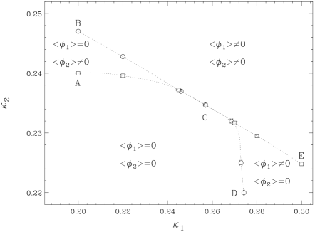
Figure 1: Phase diagram at $\lambda_{1}=0.3375,~{}\lambda_{2}=0.01125,~{}\lambda=-0.112$.

The phase diagram of the model (8) (at $T=0$), for fixed values of $\lambda_{1}$, $\lambda_{2}$ and $\lambda$, is shown in Fig. 1.

There are four distinct phases separated by four critical lines A, B, D and E: the disordered one corresponds to the lower left corner of the picture, while the upper right corner represents the totally ordered phase. The wedges in between them are partially ordered phases: in the left wedge the field $\phi_{2}$ is ordered, while $\phi_{1}$ is disordered; in the right wedge it occurs the contrary.

If there was no interaction between $\phi_{1}$ and $\phi_{2}$, we would have two independent $\phi^{4}$ models and then the critical lines would all be of second order. The lines A and E would form a straight line parallel to the $\kappa_{1}$ axis, and similarly the lines B and D would form a straight line parallel to the $\kappa_{2}$ axis. The presence of the interaction bends them as can be seen in the Figure. We managed to determine the order of the critical lines only at some distance from the region C, where the four lines merge together. The critical line A is the only one that we studied accurately: away from C, it is of second order and we observed for it Gaussian critical exponents, as it had to be expected from triviality. As for the remaining critical lines, there is a clear evidence that D is of second order, while B and E appear to be of first order. Close to C, things become unclear: while on small lattices it becomes impossible to distinguish the various phase transitions, on large ones the onset of strong metastabilities prevented us from getting any indications at all.

Understanding the phase diagram in the neighbourhood of C is of course extremely important. An important issue to address is whether the four critical lines actually meet at a single point, a double critical point that we will call ${\cal C}$, and what is its order.

Indeed, the indications coming from perturbation theory suggest that, when $g^{R}$ is negative, as required for ISB or SNR to occur, ${\cal C}$, if it exists, should be a first order critical point. This can be seen by integrating the one-loop renormalization group equations (RGE), in the scaling limit of large correlation lengths $\xi_{i}$ for both fields

$$\xi_{i}=c_{i}\;\xi\;,\;\;\;\;\xi\gg 1,$$

where $c_{i}$ are constants. In this limit the RGE of our model read:

$$\frac{dg_{1}^{R}}{dt} = -\frac{3}{16\pi^{2}}[(g_{1}^{R})^{2}+(g^{R})^{2}]\;,$$

$$\ \frac{dg_{2}^{R}}{dt} = -\frac{3}{16\pi^{2}}[(g_{2}^{R})^{2}+(g^{R})^{2}]\;,$$

$$\frac{dg^{R}}{dt} = -\frac{1}{16\pi^{2}}(g_{1}^{R}+g_{2}^{R}+4g^{R})g^{R}\;,$$ (9)

where $t=\log\xi$. Numerical integration of these equations shows that, if one starts from a set of initial values for the renormalized couplings with $g^{R}$ negative, $g_{1}^{R}$ and $g_{2}^{R}$ are driven by $g^{R}$ towards negative values in a finite interval of $t$, something that is generally believed to indicate a first-order phase transition. The fact that for negative values for the coupling $g^{R}$ the double critical point really is of first order, is shown in ref.[18], where the phase diagram of our model is studied, using a suitable truncation of the exact non-perturbative flow equations, for the particular case $g_{1}^{(0)}=g_{2}^{(0)},\;m_{1}^{(0)2}=m_{2}^{(0)2}$, when an extra $\phi_{1}\leftrightarrow\phi_{2}$ symmetry is present (this case is not directly related to ISB or SNR because this extra symmetry excludes a priori the possibility of these phenomena).

If this picture of the double phase transition for $g^{R}<0$ turns out to be correct, one may question whether in this case such a model can be used at all as an elementary particles theory. The answer to this question depends on the actual strength of the first-order phase transition. The fact that the correlation lengths of one or both fields remain finite near $\cal C$ is not necessarily a problem per se. In fact, even if $\cal C$ were of second order for both fields, triviality would prevent one from taking the correlation lengths to infinity anyway. Thus, the relevant question is to see if the correlation lengths become sufficiently large near $\cal C$, for the presence of the lattice cut-off to become negligible in low-energy amplitudes. This in turn depends on the absolute magnitude of the coupling constants. For small couplings, $\cal C$ should be only weakly first order and one should be able to achieve large correlation lengths for both fields. In realistic particle models for ISB and SNR the problem may be more serious: the presence of gauge couplings, that work in favour of symmetry restoration, usually forces one to take large negative couplings $g^{R}$, for ISB or SNR to occur [11], and this can then give rise to rather strong first order phase transitions in the scalar sector, thus spoiling the model.

3 High-T perturbation theory

In this Section we briefly review the predictions of perturbation theory on the high-temperature behavior of the model (1). We shall see that, for certain choices of the couplings, the symmetric vacuum of the theory becomes unstable at sufficiently high temperatures. In order to explore this phenomenon, we need to compute the leading high-$T$ contribution to the second derivatives of the effective potential in the origin, or equivalently the 1PI 2-point functions for zero external momenta $p$. A standard one-loop computation (in the imaginary time formalism) [19] in our model gives the result:

$$M_{1}^{2}(T) \equiv -\Gamma^{(2)}_{1}(p=0,T)=m_{1}^{2}+\frac{T^{2}}{24}\left[g_{1}^{R}h\left(\frac{m_{1}}{T}\right)+g^{R}h\left(\frac{m_{2}}{T}\right)\right]~{}~{},$$

$$M_{2}^{2}(T) \equiv -\Gamma^{(2)}_{2}(p=0,T)=m_{2}^{2}+\frac{T^{2}}{24}\left[g_{2}^{R}h\left(\frac{m_{2}}{T}\right)+g^{R}h\left(\frac{m_{1}}{T}\right)\right]~{}~{},$$ (10)

where $m_{i}^{2}$ represent the renormalized masses at $T=0$ and $h(x)$ is the function:

$$h(x)=\frac{6}{\pi^{2}}\int_{0}^{\infty}dy\;\frac{y^{2}}{(x^{2}+y^{2})^{1/2}(e^{(x^{2}+y^{2})^{1/2}}-1)}~{}.$$ (11)

It is clear that $h(x)$ is positive, monotonically decreasing and that it approaches zero when $x\rightarrow\infty$. For small values of $x$, $h(x)$ has the asymptotic expansion:

$$h(x)=1-\frac{3}{\pi}x-\frac{3}{2\pi^{2}}x^{2}\left(\ln\frac{x}{4\pi}+\gamma-\frac{1}{2}\right),$$ (12)

$\gamma$ being the Euler constant. In the limit of very high-temperatures $m_{i}/T\ll 1$, eqs.(10) reduce to:

$$M_{1}^{2}(T)=m_{1}^{2}+\frac{T^{2}}{24}(g_{1}^{R}+g^{R})~{}~{},$$

$$M_{2}^{2}(T)=m_{2}^{2}+\frac{T^{2}}{24}(g_{2}^{R}+g^{R})~{}~{}.$$ (13)

Assuming for simplicity that the bare couplings are so small that they can be identified with the renormalized ones, and recalling that the coupling $g^{(0)}\approx g^{R}$ can be negative, it is easy to see that for $g_{1}^{R}/g_{2}^{R}$ sufficiently large, the range (2) of stability for the potential includes values of $g^{R}$ such that, say, $g_{2}^{R}+g^{R}$ is negative (it can be proven easily form eqs.(2) that one cannot have $g_{1}^{R}+g^{R}<0$ at the same time). In this case we see from eq.(13) that $M_{2}^{2}(T)$ becomes negative at sufficiently high temperatures, irrespective of its value at $T=0$. This is the essence of the phenomena of SNR and ISB: in multiscalar models some Debye masses can become negative and so one can have spontaneous symmetry breaking at arbitrarily high temperatures. We now focuse on ISB, the phenomenon to be explored in this paper: in this case we take $m_{1}^{2}>0,\;m_{2}^{2}>0$, so that the vacuum is disordered at $T=0$, and again assume that $g_{2}^{R}+g^{R}<0$. If one starts increasing the temperature, it will happen that, at a certain critical temperature $T_{c}$, the field $\phi_{2}$ will undergo spontaneous symmetry breaking and will stay broken at all higher temperatures. The field $\phi_{1}$, instead, will remain disordered. The critical temperature $T_{c}$ can be estimated from eq.(13) to be:

$$\frac{T_{c}}{m_{2}}=\sqrt{-\frac{24}{g^{R}+g_{2}^{R}}}\;\;.$$ (14)

Even though they capture the main features of ISB and SNR, at a closer inspection, eqs.(13) and (14) appear unsatisfactory in two respects. First of all, the condition for the high-T instability in, say, the $\phi_{2}$ direction, $g_{2}^{R}+g^{R}<0$, as deduced from the second of eqs.(13), does not involve $g_{1}^{R}$. Since the bound (2), together with the condition $g_{2}^{R}+g^{R}<0$, typically implies a hierarchy among the couplings $g_{1}^{R}\gg|g^{R}|\geq g_{2}^{R}$, it is clear that next-to-leading order corrections involving $g_{1}^{R}$ can produce significant corrections to the lowest order result. The second fault of eqs.(13) and (14) is the most important for our study of ISB. It is the fact that the estimate (14) of the critical temperature does not involve $m_{1}^{2}$: this looks physically incorrect, for one can imagine that for $m_{1}\gg m_{2}$ the field $\phi_{1}$ should decouple from $\phi_{2}$ for temperatures $T\ll m_{1}$ and so ISB or SNR should not occur before the scale $m_{1}$ is reached. Both limitations of the one-loop picture can be overcome by performing the resummation of the so called ring diagrams.

As it is well known [17], these diagrams represent the dominant next-to-leading corrections at high temperatures and their inclusion leads to a more accurate description of both the phase transition and the high temperature behavior of the thermal masses. This infinite resummation leads to self-consistent gap equations for the Debye masses $M_{i}^{2}(T)$, which in our case read

$$x_{1}^{2} = \frac{m_{1}^{2}}{T^{2}}+\frac{g_{1}^{R}}{24}h(x_{1})+\frac{g^{R}}{24}h(x_{2})~{}~{},$$

$$x_{2}^{2} = \frac{m_{2}^{2}}{T^{2}}+\frac{g_{2}^{R}}{24}h(x_{2})+\frac{g^{R}}{24}h(x_{1})~{}~{},$$ (15)

where we defined $x_{i}=M_{i}(T)/T$. For any given temperature $T$, the symmetric vacuum is stable if the above equations admit real (positive) solutions for $x_{i}$. At sufficiently low temperatures, this is clearly the case if we take $m_{1}^{2}>0,\;m_{2}^{2}>0$. One can now gradually increase $T$ and follow the evolution of $x_{1}$ and $x_{2}$: if one of them, say $x_{2}$, approaches zero at $T=T_{c}$, and if for $T>T_{c}$ the gap equations do not admit anymore real solutions, one can argue that for $T>T_{c}$ there will be ISB in the $\phi_{2}$ direction. It is clear that this can happen only if $g^{R}$ is negative and its absolute value is large enough in comparison with $g_{2}^{R}$. A detailed study of the conditions required is given in the first of refs.[11], where it is shown that the parameter region for which ISB or SNR occur is indeed smaller than that predicted by the naive eqs.(13). An analogous result was later confirmed by studies based on different non-perturbative techniques [12].

Assuming now that at high temperatures there develops an instability in the $\phi_{2}$ direction, a better estimate of the critical temperature $T_{c}$, than that given by the one-loop equations (14), can be obtained by setting $x_{2}=0$ in eqs.(15) and then solving the system:

$$x_{1}^{2} = \frac{m_{1}^{2}}{T_{c}^{2}}+\frac{1}{24}(g_{1}^{R}h(x_{1})+{g^{R}})~{}~{},$$

$$0 = \frac{m_{2}^{2}}{T_{c}^{2}}+\frac{1}{24}(g_{2}^{R}+g^{R}h(x_{1}))~{}~{},$$ (16)

where we have used $h(0)=1$. Upon comparing the second of eqs.(16) with the second of eqs.(13), it is clear that the inclusion of the ring diagrams pushes the phase transition to higher temperatures. This is so because the negative coupling $g^{R}$, which is the cause of ISB, comes with the factor $h(x_{1})$, which is always less than one. Since $x_{1}$ is larger then $m_{1}^{2}/T_{c}^{2}$, as it is clear from the first of eqs.(16), we see that a large mass $m_{1}^{2}$ will make ISB harder to achieve. In fact, the influence of $m_{1}^{2}$ can be so strong as to cause the disappearance of the symmetry-breaking phase transition predicted by the one-loop formula. As we shall explain in greater detail in Sec. 6, this effect probably explains why we did not observe ISB in our previous work [15].

4 ISB on the lattice

We saw in the previous Section that, for $g_{2}^{R}+g^{R}$ sufficiently negative, continuum perturbation theory predicts ISB for the $\phi_{2}$ field. Even if the mass parameters are chosen in such a way that the ground state is disordered at $T=0$, the field $\phi_{2}$ should develop a non-vanishing vev above some critical temperature $T_{c}$ and should remain ordered at all higher temperatures. The field $\phi_{1}$, instead, should remain disordered.

In principle it is very simple to study ISB on the lattice. As it is well known, finite temperatures are simulated by lattices with a finite extension in the “time” direction (and infinite extension in the remaining “space” directions, as required by the thermodynamic limit), the temperature being related to the number $N_{t}$ of sites by the relation:

$$T=\frac{1}{N_{t}a}\;,$$ (17)

with $a$ the lattice spacing. So, in order to study ISB, one should simply check how the critical lines of the $T=0$ phase diagram, shown in Fig.1, shift in the $(\kappa_{1},\kappa_{2})$ plane (for fixed values of $\lambda_{1}$, $\lambda_{2}$ and $\lambda$) as a function of the temperature, which means concretely as a function of $N_{t}$ (in principle, one could vary the temperature also by varying the lattice spacing in the time direction, but we have not used this method). Since we are specifically interested in the behavior of the field $\phi_{2}$, it is sufficient to focuse our attention on the critical line of this field, the line A-E of Fig.1. If, for the selected values of $\lambda_{1}$, $\lambda_{2}$ and $\lambda$, ISB occurs, it should happen that, when the temperature is increased, namely when $N_{t}$ is diminished, the $\phi_{2}$-critical line penetrates more and more deeply in the disordered region of the $T=0$ phase diagram, at least in a neighbourhood of the double critical point ${\cal C}$. The effect should be clearest at the highest temperatures, i.e. for the smallest values of $N_{t}$. To help the reader visualize the situation, we have shown in Fig.2 the expected $N_{t}$-behavior of the $\phi_{2}$-critical line, in case of ISB. Some comments are in order.

Figure 2: Expected (qualitative) temperature-behavior of the critical line for the $\phi_{2}$ transition, in case of ISB. The region studied by us is the one to the left of C.

We expect that far from the double critical point ${\cal C}$ the $N_{t}$ behavior of the $\phi_{2}$-critical line should always be the normal one, namely the critical line should move towards greater values of $\kappa_{2}$ when $N_{t}$ is diminished. This conjecture looks reasonable, if one considers that far from $\cal C$, the field $\phi_{1}$ should be far from critical and its correlation length should become very small. This implies that the influence of the field $\phi_{1}$ over the field $\phi_{2}$, near the critical line of the latter, should be negligible and so the behavior of $\phi_{2}$ should be that of a normal $\phi^{4}$ theory, where an increase of temperature shifts the transition upwards. This means that ISB should be visible, if it happens at all, only close enough to ${\cal C}$, in the scaling region where the correlation lengths of both fields become large. This explains why, in Fig. 2, we have drawn the critical lines for $N_{t}=2,3,4,5$ below that of the $T=0$ theory ($N_{t}=\infty$) only near ${\cal C}$, while away from ${\cal C}$ they all lie above it.

Such a behavior poses a very serious problem: imagine that for the few values of $N_{t}$ simulated, one has found a result like that shown in Fig. 2, which supports ISB. How can one convince oneself that nothing will change for greater values of $N_{t}$? One could suspect that for $N_{t}$ large enough the critical line might pass entirely above that of the $T=0$ theory, thus leading to the disappearance of ISB. In practice, it is then very important to have a criterion to decide if, whatever behavior is observed with the few $N_{t}$’s that are simulated, it will not change when going to higher $N_{t}$’s. The common practice to address this question is to search for scaling in the $N_{t}$ dependence of some observable: this is what we did in [15], where, for a fixed value of $\kappa_{1}$ and several values of $N_{t}$, we measured the critical values of $\kappa_{2}$, $\kappa_{2}^{c}(N_{t})$. The values we got were all greater than the critical value $\kappa_{2}^{c}$ for $T=0$, a result against ISB (very likely, the value of $\kappa_{1}$ used for the simulations in [15] was too far from ${\cal C}$, for ISB to be visible. We were probably in the region of Fig. 2 on the left of ${\cal C}$, where the behavior of the $\phi_{2}$ critical line becomes the “normal” one. We shall have more to say on this in Sec. 6.) . The good scaling of $\kappa_{2}^{c}(N_{t})$ with $N_{t}$ convinced us that no change would have occurred for larger $N_{t}$. We think that applying this method to make sure that ISB survives for all values of $N_{t}$ would be very difficult, because we believe that in order to observe ISB for a number of values of $N_{t}$ large enough for a scaling analysis to be possible, one needs look very close to the critical point ${\cal C}$, where the large correlation lengths make it necessary to use very large lattices for a reliable measurement of the critical couplings.

$N_{t}$	$N_{s}$	# runs	Thermalization sweeps	# sweeps
2	6	1	$5\times 10^{4}$	$4\times 10^{6}$
2	8	1	$10^{5}$	$8\times 10^{6}$
2	10	1	$2\times 10^{5}$	$10^{7}$
2	12	1	$3\times 10^{5}$	$10^{7}$
2	16	2	$2\times 10^{5}$	$8\times 10^{6}$
2	20	4	$8\times 10^{4}$	$6.4\times 10^{6}$
6	6	1	$5\times 10^{4}$	$4\times 10^{6}$
8	8	1	$10^{5}$	$8\times 10^{6}$
10	10	1	$2\times 10^{5}$	$4\times 10^{6}$
12	12	1	$3\times 10^{5}$	$8\times 10^{6}$
16	16	4	$2\times 10^{5}$	$9.6\times 10^{6}$
20	20	6	$2.4\times 10^{5}$	$9.6\times 10^{6}$

Table 1: Statistics for the simulations on lattices of sizes $N_{t}\times N_{s}^{3}$.

As a matter of fact, in the new series of simulations presented here, we have been able to simulate only one value of $N_{t}$, $N_{t}=2$, and we needed a very large statistics in order to detect reliably the shift of the $\phi_{2}$ critical line.

Let us briefly explain the method we have followed, postponing the details to the next two subsections.

The first part of the method is exactly the same as that of ref.[15], but it is useful to review it here again. We fixed once and for all a set of values for $\lambda_{1},\lambda_{2}$ and $\lambda$. This time, we took $\lambda_{1}=0.16875$, $\lambda_{2}=0.0001125$, $\lambda=-0.00784$. There are two important differences with ref.[15]:

a) the new values of the couplings are smaller than the old ones [15]. This was done to be closer to the perturbative region, but it increased tremendously the difficulty of the simulations, because the shift of the critical line with $N_{t}$ was this time much smaller than before;

b) more importantly, the ratio $|\lambda|/\lambda_{2}$ is now much greater than before (more or less 70 against 10), and so there is now a much stronger push towards ISB.

After a quick analysis of the phase diagram at $T=0$, we selected a value of $\kappa_{1}$, $\kappa_{1}=0.24$, to the left of $\cal C$, and then we measured accurately the corresponding critical value $\kappa_{2}^{c}$ of $\kappa_{2}$ along the $\phi_{2}$ critical line, always at $T=0$.

Near this point, we measured the $T=0$ values of the renormalized couplings and the correlation lengths of both fields, for the same value of $\kappa_{1}$, but for a value of $\kappa_{2}$ slightly less than $\kappa_{2}^{c}$, in the disordered phase (the results of these measurements are given in Table 2). The value of $\xi_{1}\simeq 1$ that we got is not very large, but still acceptable for us to believe that we were probing the continuum region. In any case, we could not achieve larger values for $\xi_{1}$, because near to ${\cal C}$ we encountered strong metastabilities that made any simulations impossible. We notice also that the value of $g_{1}^{R}$ is quite large and not very accurate; on the contrary, what we think is the essential, we see that $g_{2}^{R}$ and $|g^{R}|$ are both very small and that the condition for ISB is implemented very strongly, since $|g^{R}|/g_{2}^{R}\simeq 10$. The one-loop formulae obviously predict that ISB should occur for these values of the couplings, and it can be checked that the ratio $|g^{R}|/g_{2}^{R}$ is large enough for ISB to survive also the inclusion of the ring diagrams. This convinced us that we had found a good simulation region.

Having performed all these measurements at $T=0$, we turned to finite values of $N_{t}$. Due to the extreme smallness of the effect, we were able to detect the shift of $\kappa_{2}^{c}$ (for $\kappa_{1}=0.24$) only for the smallest value of $N_{t}$, $N_{t}=2$. Even in this case, the shift was of the order of one part in hundred thousands and so larger values on $N_{t}$ look out of reach. Since this shift turned out to be towards smaller values of $\kappa_{2}$, our result can be considered as favourable to ISB.

In the next two Subsections, we describe the details of the numerical simulations and how we managed to measure the critical values of $\kappa_{2}$ with the high accuracy that was needed.

4.1 MC Simulation: determination of $\kappa_{2}^{c}$

Figure 3: Binder cumulants for the $2\times N_{s}^{3}$ lattices ($N_{s}=6,8,10,12,16,20$) at $\lambda_{1}=0.16875,~{}\lambda_{2}=0.0001125,~{}\lambda=-0.00784$ and $\kappa_{1}=0.24$.

For this new simulation, we used the Metropolis Algorithm (cluster was not efficient), with $3$ hits and acceptance around $60\%$. We simulated lattices of sizes $2\times N_{s}^{3}$ and $N_{s}^{4}$, with $N_{s}=6,8,10,12,16,20$. In the new region of parameters the field fluctuations are strong and the transitions for different lattice sizes are very close. We had to accumulate very large statistics in order to obtain accurate results. In Table 1 we summarize the statistics for every lattice: number of runs, sweeps left for thermalization and total number of sweeps for every run.

As we said above, all our simulations were performed for a single value of $\kappa_{1}$, $\bar{\kappa}_{1}$=$0.24$. A fast simulation on the $6^{4}$ lattice gave us the approximate position, $\kappa_{2}=0.24903$, of the phase transition of the field $\phi_{2}$ (the field $\phi_{1}$ remains disordered across the transition). All the subsequent massive simulations were performed at this point, and the results were extrapolated in a narrow $\kappa_{2}$-interval around it by means of the Spectral Density Method [22] (SDM). The observable used to locate with high precision the phase transition was the Binder cumulant:

$$U_{i}(N_{s},\kappa_{1},\kappa_{2})=\frac{3}{2}-\frac{\langle M_{i}^{4}\rangle}{2\langle M_{i}^{2}\rangle^{2}}~{},$$ (18)

where $M_{i}$ stands for the magnetization of the field $\phi_{i}$.

Figs.3 and 4 show the values of $U_{2}$ obtained by extrapolating the results of the simulations by means of the SDM. Every pair of curves ($N_{s}$ and $\hat{N_{s}}$) determines a crossing point, that gives an estimate $\kappa_{2}^{*}(N_{s},\hat{N_{s}})$ of the critical point $\kappa_{2}^{c}$. These values do not suffer from finite size effects, except for corrections to scaling, which can be parametrized and used to obtain $\kappa_{2}^{c}$, according to the scaling law:

$$\kappa^{*}_{2}(N_{s},bN_{s})-\kappa_{2}^{c}=\frac{1-b^{-\omega}}{b^{1/\nu}-1}N_{s}^{-\omega-1/\nu}~{},$$ (19)

where $\omega$ is the exponent for the corrections to scaling. In the calculation of the error, due account was taken of the fact that the pair crossings were not all independent of each other (out of the $N(N-1)/2$ crossings between $N$ curves, only $2N-3$ are independent of each other).

As for the exponents occurring in eq. (19), we had to distinguish the symmetric ($N_{s}^{4}$) lattices from the asymmetric ($2\times N_{s}^{3}$) ones. In the case of the latter, since the scaling parameter is $N_{s}$, while $N_{t}$ is fixed, according to the hypothesis of dimensional reduction and universality, we used the exponents of the Ising model in three dimensions, namely $\nu=0.63$ and $\omega=0.8$. As a check, we also computed $\nu$ directly from the data obtaining values fully compatible with the above one (see Fig. 7).

Figure 4: Binder cumulants for the $N_{s}^{4}$ lattices ($N_{s}=6,8,10,12,16,20$) at $\lambda_{1}=0.16875,~{}\lambda_{2}=0.0001125,~{}\lambda=-0.00784$ and $\kappa_{1}=0.24$.

In the case of the symmetric lattices, we used the mean field exponents $\omega=0,\nu=1/2$. As seen from eq.(19), these values imply that, apart from logarithmic corrections, all the crossings should occur for the same value of $\kappa_{2}$, and this is approximately what we found. A better estimate of $\kappa_{2}^{c}$ was then obtained by setting $\omega\neq 0$ in eq.(19) and taking the limit, for $\omega\to 0$, of the corresponding values of $\kappa_{2}^{c}$. In the process, we observed a very fast convergence.

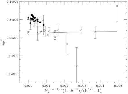
Figure 5: Fits to obtain $\kappa_{2}^{c}$ from the crossings of the Binder cumulants. The results are $\kappa_{2}^{c}(T=0)=0.249022(2)$ (filled) and $\kappa_{2}^{c}(N_{t}=2)=0.249005(2)$ (empty).

The result of the extrapolation for $N_{s}\to\infty$ is shown in Fig. 5. We got $\kappa_{2}^{c}(N_{t}=2)=0.249005(2)$ and $\kappa_{2}^{c}(T=0)=0.249022(2)$. This means that the disordered region diminishes when $T$ is increased, as ISB requires, at least for the case of the highest temperature reachable on the lattice ($N_{t}=2$).

4.2 MC Simulation: maximum of the Binder cumulant derivative

Due to the extreme smallness of the shift in the value of $\kappa_{2}^{c}$, we found it opportune to compute the two values of $\kappa_{2}^{c}$ also in another way, completely independent on the previous one. Indeed, for every value of $N_{s}$, one can determine the point $\kappa_{2}^{**}(N_{s})$ where the derivative $\partial U_{2}/\partial\kappa_{2}$ reaches its maximum value, namely $C_{v}$. It is well known that, in the limit $N_{s}\rightarrow\infty$, $\kappa_{2}^{**}(N_{s})$ approaches $\kappa_{2}^{c}$ according to the scaling law (including corrections to scaling):

$$\kappa_{2}^{**}(N_{s})-\kappa_{2}^{c}\propto N_{s}^{-1/\nu}(1-AN_{s}^{-\omega})\,$$ (20)

which allows us to compute $\kappa_{2}^{c}$. Fig.6 shows the corresponding fits. In this computation, we used the same critical exponents discussed in the previous subsection. We obtained $\kappa_{2}^{c}(N_{t}=2)=0.248997(11)$ and $\kappa_{2}^{c}(T=0)=0.249017(2)$, which are fully compatible with the previous results.

As a final check, we computed $\nu$ from the maximum of $\partial U_{i}/\partial\kappa_{2}$, $C_{v}$, which diverges with the lattice size as $N_{s}^{1/\nu}$. Again, we obtained consistent results, as can be seen in Fig. 7.

Figure 6: Fits to obtain $\kappa_{2}^{c}$ from the maximum of the Binder cumulant derivative. (The exponents used were $\nu=0.63,\omega=0.8$ for $N_{t}=2$ and $\nu=1/2$ for $N_{t}=N_{s}$).

Figure 7: Fits to obtain $\nu$ by using the maximum of the Binder cumulant derivative.

In conclusion, this time, differently from what we reported in [15], we found that, when $N_{t}=2$, the phase transition of the field $\phi_{2}$ occurs for a value of $\kappa_{2}$ which is smaller than at $T=0$. The two measures of $\kappa_{2}^{c}$ took a long time, because, for the small values of $\lambda_{2}$ and $\lambda$ used now, the shift of the critical $\phi_{2}$-line is extremely small and we had to measure both values of $\kappa_{2}^{c}$ with six significant digits, a job that took us months of computer time!

So, the results of our new simulations are favourable to ISB, but cannot be considered as conclusive because they refer to a single value of $N_{t}$.

5 Comparison with Perturbation theory

As we said in Section 3, simulating only a finite number of $N_{t}$ values is per se not sufficient to claim ISB, for one cannot rule out the possibility that the phenomenon would disappear for larger values of $N_{t}$. In fact, the case here is even worse, since we have at our disposal just one value of $N_{t}$, $N_{t}=2$. In order to increase confidence in our result, we attempted a comparison of our MC data with the perturbative predictions. While the one-loop formulae, eqs.(14), lead to an estimate of the critical temperature far from the MC value, we found a reasonable agreement with the predictions of the gap equations, eqs.(16).

$N_{s}$	$\xi_{1}$	$\xi_{2}$	$g_{1}^{R}$	$g_{2}^{R}$	$g^{R}$
6	0.9581(2)	10.78(1)	26(6)	0.0261(9)	-0.35(1)
8	0.9528(3)	11.48(2)	41(11)	0.0296(15)	-0.29(1)

Table 2: $T=0$ values of the correlation lengths and renormalized couplings for $\kappa_{1}=\bar{\kappa}_{1}\equiv 0.24$, $\kappa_{2}=\bar{\bar{\kappa}}_{2}\equiv 0.2488$ (lattice sizes $N_{s}^{4}$).

We shall now explain how this comparison was done. Let $p=(\bar{\kappa}_{1},\bar{\kappa}_{2})$ be the point of the $\phi_{2}$-critical line for $N_{t}=2$, that we identified in our simulations. As we saw, $p$ belongs to the disordered phase of the $T=0$ phase diagram. If we knew the $T=0$ values of the renormalized couplings and correlation lengths $\xi_{1}$ and $\xi_{2}$ (we measure them in units of the lattice spacing) at $p$, we could get an estimate of the critical inverse temperature $N_{t}^{c}$ by solving eq.(14) or eqs.(16), since

$$\left(\frac{T_{c}}{m_{i}}\right)^{MC}=\frac{\xi_{i}}{N_{t}^{c}}~{}.$$ (21)

If perturbation theory works, we should get for $N_{t}^{c}$ a value close to two.

This procedure, even if simple from the conceptual point of view, is difficult to carry out: since $p$ is very close to the critical line of the $T=0$ phase diagram, the correlation length $\xi_{2}$ is huge there (in our case, we estimate it to be larger than 40). Thus a measure of the $T=0$ renormalized couplings and correlation lengths at $p$ requires 4d-lattices with $N_{s}\geq 40$, which is just too much for computers available today.

In order to avoid the difficulties connected with exceedingly large correlation lengths for the field $\phi_{2}$, we measured the renormalized couplings and the correlation lengths (for $T=0$) at a point $\bar{p}=(\bar{\kappa}_{1},\bar{\bar{\kappa}}_{2})$, having the same $\kappa_{1}$ coordinate as $p$, but with $\bar{\bar{\kappa}}_{2}$ slightly less than ${\bar{\kappa}}_{2}$, and such that $\xi_{2}$ was more or less ten (see Table 2). Because of time limitations, we did not carry out the thermodynamic limit in this series of measures and contented ourselves with simple estimates on rather small lattices. The quantitative considerations that follow have to be taken, then, as simply indicative.

Afterwards, we computed the values of $g_{1}^{R}$, $g_{2}^{R}$, $g_{R}$ and of $\xi_{1}$ and $\xi_{2}$ at $p$, by integrating a set of ($T=0$) RGE’s in the interval $\bar{\bar{\kappa}}_{2}<\kappa_{2}<\bar{\kappa}_{2}$. We evaluated the $\beta$-functions to two-loops order, following a procedure strictly analogous to that discussed in [20]. Of course in our case there was a larger number of $\beta$ functions to be computed. Since the value of $\xi_{1}$ at $\bar{p}$ was only roughly one, we included in our $\beta$-functions the corrections to scaling upto one-loop order.

The reader might question the reliability of these perturbative RGE’s, since the value of $g_{1}^{R}$ at $\bar{p}$ is rather large and quite uncertain. We believe that this is not a problem, for two reasons. The first one is that the integration interval in $\kappa_{2}$ is very small. The second, and most important, is less obvious: it turns out that $g_{1}^{R}$ does not appear in any of the $\beta$ functions (at least to the two-loops order that we have examined). Its absence can be understood by considering that, since we are moving in the vertical direction in the $(\kappa_{1},~{}\kappa_{2})$ plane, $\xi_{1}$ remains finite (and practically constant).

After the numerical integration, it turned out that the running of $g_{1}^{R}$, $g_{2}^{R}$, $g^{R}$ and $\xi_{1}$ in the tiny $\kappa_{2}$ interval considered was completely negligible, while $\xi_{2}$ varied from 11 to something like 45. Since the final value of $\xi_{2}$ was very sensitive to its initial value, (and practically insensitive to the initial values of the other parameters), we took advantage of our accurate knowledge of $\kappa_{2}^{c}(T=0)$, and tuned the initial value of $\xi_{2}$ in such a way that $\kappa_{2}$ would approach the MC value of $\kappa_{2}^{c}(T=0)$ in the limit $\xi_{2}\rightarrow\infty$. The initial value of $\xi_{2}$ that we obtained in this way, $\xi_{2}=11.85(5)$, is very close to the MC one, as can be seen from Table 2. The value of $\xi_{2}$ at $p$ turned out to be $\xi_{2}(p)=45(5)$: the error is basically due to the uncertainty in the MC values of $\kappa_{2}^{c}(T=0)$ and $\kappa_{2}^{c}(N_{t}=2)$.

We thus solved eq.(14) and eqs.(16) with respect to $N_{t}^{c}$, using as inputs the values of $g_{1}^{R}$, $g_{2}^{R}$, $g^{R}$ and $\xi_{1}$ given in Table 2 and the above value of $\xi_{2}(p)$. In this way we obtained the following estimates of $N_{t}^{c}$:

$$N_{t}^{c({\rm one-loop})}=4.8(6)\;,\;\;\;\;\;\;\;N_{t}^{c({\rm gap})}=1.7(2).$$ (22)

It is clear that $N_{t}^{c({\rm one-loop})}$ is far from the MC value $N_{t}=2$, while $N_{t}^{c(gap)}$ is quite close. It seems, then, that resummed perturbation theory provides a rather accurate description of our data.

6 Some comments about recent results on ISB on the Lattice

Recently, there have been two other MC studies of ISB in four dimensions, one by our group [15] and another by Jansen and Laine [16]. While in the first one no sign of ISB was found, the latter authors claimed to have seen clear evidence of ISB and good agreement with resummed perturbation theory. We would like to make here a few comments on these works.

We shall start from our own previous work. The method followed there was very similar to that used in this paper, but the simulations were performed for a different choice of parameters. We think now that the essential reason for the negative result is the fact that the conditions for ISB were not enforced strongly enough. Near the simulation point, the absolute value of $g^{R}$ was roughly the double of the value of $g_{2}^{R}$: according to the one loop formulae (13), this was more than enough to induce ISB, but nevertheless we did not find it. The reason of the failure is hidden in the gap equations (15). Near our simulation point the correlation length of $\phi_{1}$ was approximately one. This implies that, even at highest temperature (corresponding to $N_{t}=2$) and so in the conditions most favourable to ISB, $m_{1}/T=N_{t}/\xi_{1}$ was approximately equal to two. By looking at the gap equations, it is easy to convince oneself that, with a value of $m_{1}/T\approx 2$, a $|g^{R}|$ which is twice $g_{2}^{R}$ is not enough to induce ISB. The reason is the suppressing factor $h(x_{1})$ in front of $g^{R}$ in the second of eqs.(15): since $x_{1}\approx 2$, and $h(2)\approx 0.17$ it is clear that one would have needed a $|g^{R}|$ at least six times bigger than $g_{2}^{R}$. In order to be on the safe side, in the new simulations presented in this paper, since $\xi_{1}$ was still of order one, we selected $|g^{R}|\approx 10\;g_{2}^{R}$ which now was large enough.

As for ref.[16], the authors searched for ISB in an $O(4)\times Z_{2}$ two scalar model. Their approach is very different from ours, and it is useful to briefly review it here. Using perturbation theory (with two-loops accuracy), they computed the relations giving the (bare) lattice parameters, in terms of the renormalized masses and couplings, in the symmetric phase of their model. Then, they performed a set of simulations on lattices with $N_{t}=2,4$ (the few short runs on symmetric lattices, according to the authors, should not be given much importance) for a number of values of the bare couplings, corresponding to decreasing values for the renormalized mass $m_{1}$ of the field expected to undergo ISB ($\phi_{1}$), and constant values for the remaining renormalized parameters. In this way they were able to vary the ratio $T/m_{1}$ in a large interval, even holding $N_{t}$ fixed, or varying it very little, by just varying the renormalized mass $m_{1}$. In the simulations they measured the expectation value of the modulus of $\phi_{1}$, and the results turned out to be fully compatible with the predictions of (resummed) perturbation theory. In particular, the field $\phi_{1}$ appeared to be disordered for values of $T/m_{1}$ small enough, and ordered for larger values of that ratio, which is a sign of ISB. Compared with our approach, this procedure presents the advantage of avoiding the very demanding task of an accurate determination of the critical point, but on the other side it is necessarily limited to the region of very small couplings, in order for perturbation theory to be applicable. Indeed, in ref.[16], perturbation theory was used not only to compute the relations between the bare and renormalised couplings, as we said above, but also to monitor the behavior of $<|\phi_{1}|>$ in the thermodynamical limit. In view of the long lasting debate, whether ISB and SNR are genuine effects or rather artifacts of perturbation theory, we preferred to pursue the approach presented in this paper which, even if much more expensive, in terms of computer time, does not make any recourse to perturbation theory. As a reward, we were able to probe much larger values of the coupling constants, something which is especially important in view of the applications of ISB to realistic cosmological scenarios, where large couplings in the scalar sector are usually needed in order to enforce ISB, as was pointed out at the end of Sec.2. Moreover, we could also study in detail the nature of the symmetry-breaking high-$T$ phase transition.

7 Conclusions

We have studied ISB at high temperature in four dimensions in a two-scalar $\phi^{4}$ model with $Z_{2}\times Z_{2}$ global symmetry. For fixed values of the coupling constants $\lambda_{1},\lambda_{2},\lambda$ and of the hopping parameter $\kappa_{1}$, we measured the critical value of the hopping parameter $\kappa_{2}$, for which the field $\phi_{2}$ undergoes spontaneous symmetry breaking. This measure was performed both at $T=0$ and at $T>0$. It was found that the value of $\kappa_{2}^{c}$ at $T>0$ is smaller than that for $T=0$, which is a signal of ISB. Due to the extreme smallness of the shift, it was necessary to measure the values of $\kappa_{2}^{c}$ with very high precision. This accuracy was reached via an accurate analysis of FSS on large lattices with very high statistics. The extreme difficulty of the measurements did not allow a scaling analysis of the dependence of the result on the number of sites $N_{t}$ in the time direction. For this reason, we cannot consider our results as conclusive.

In order to increase our confidence in the result, we compared the MC value of the critical temperature $T_{c}$ with the theoretical value. While the simple one-loop estimate turned out to be grossly incorrect, we found a reasonable agreement with the value of $T_{c}$ obtained from the gap equations (16), which result from the resummation of the ring diagrams.

So, in conclusion, we have found some evidence that ISB is possible and that resummed perturbation theory provides a qualitatively correct description of the phenomenon. Nevertheless, we think that our results are not conclusive and that further work is needed before ISB can be claimed with confidence.

References

- [1] S. Weinberg, Phys. Rev. D 9 (1974) 3357.
- [2] R.N. Mohapatra and G. Senjanović, Phys. Lett. B 89 (1979) 57; Phys. Rev. Lett. 42 (1979) 1651; Phys. Rev. D 20 (1979) 3390.
-
[3]
P. Salomonson, B.-S. Skagerstam and A. Stern, Phys. Lett.
B 151 (1985) 243;
G. Dvali, A. Melfo and G. Senjanović, Phys. Rev. Lett. 75 (1996) 4559;
G. Dvali and G. Senjanović, Phys. Rev. Lett. 74 (1995) 5178;
P. Langacker and S.-Y. Pi, Phys. Rev. Lett. 45 (1980) 1. -
[4]
S. Dodelson and L. Widrow, Mod. Phys. Lett A 5 (1990) 1623;
Phys. Rev. D 42 (1990) 326; Phys. Rev. Lett. 64 (1990) 340;
S.Dodelson, B.R. Greene and L.M. Widrow, Nucl. Phys. B 372 (1992) 347. - [5] J. Lee and I. Koh, Phys. Rev. D 54 (1996) 7153.
- [6] G. Dvali, A. Melfo and G. Senjanović, Phys. Rev. D 54 (1996) 7857.
-
[7]
G. Dvali and K. Tamvakis, Phys. Lett. B 378 (1996) 141;
B. Bajc and G. Senjanović, Nucl. Phys. Proc. Suppl.52A (1997) 246;
A. Riotto and G. Senjanović, Phys. Rev. Lett. 79 (1997) 349;
A. Riotto, Nucl. Phys. Proc. Suppl. 62 (1998) 253;
B. Bajc, “Susy and symmetry nonrestoration at high temperature”, hep-ph/9902470. -
[8]
Y. Fujimoto and S. Sakakibara, Phys. Lett. B 151 (1985) 260;
E. Manesis and S. Sakakibara, Phys. Lett. B 157 (1985) 287;
K. G. Klimenko, Theor. Math. Phys. 80 (1989) 929;
M.P. Grabowski, Z.Phys. C 48 (1990) 505;
J. Orloff, Phys. Lett. B 403 (1997) 309. -
[9]
G.A. Hajj and P.N. Stevenson, Phys. Rev. D 37 (1988) 413;
K.G.Klimenko, Z.Phys. C 43 (1989) 581. - [10] Y. Fujimoto, A. Wipf and H. Yoneyama, Z. Phys. C 35 (1987) 351; Phys. Rev. D 38 (1988) 2625.
-
[11]
G. Bimonte and G. Lozano,
Phys. Lett. B 366 (1996) 248; Nucl. Phys. B 460 (1996) 155;
G. Amelino-Camelia, Phys. Lett. B 388 (1996) 776; Nucl. Phys. B 476 (1996) 255. -
[12]
T. Ross, Phys. Rev. D 54 (1996) 2944;
M. Pietroni, N. Rius and N. Tetradis, Phys. Lett. B 397 (1997) 119. - [13] M.B. Gavela, O. Pne, N. Rius and S. Vargas-Castrillón, Phys. Rev. D 59 (1998) 25008.
- [14] G. Bimonte, D. Iñiguez, A. Tarancón and C.L. Ullod, Nucl. Phys. B 490 (1997) 701.
- [15] G. Bimonte, D. Iñiguez, A. Tarancón and C.L. Ullod, Phys. Rev. Lett. 81 (1998) 750.
- [16] K. Jansen and M. Laine, Phys. Lett. B 435 (1998) 166.
- [17] L. Dolan and R. Jackiw, Phys. Rev. D 9 (1974) 3320.
- [18] S. Bornholdt, N. Tetradis and C. Wetterich, Phys. Lett. B 348 (1995) 89.
- [19] J.I. Kapusta, Finite temperature Field Theory (Cambridge University Press, Cambridge, 1989).
- [20] M. Lscher and P. Weisz, Nucl. Phys. B 290 (1987) 25.
- [21] K. Binder, Z. Phys. 43 (1981) 119.
- [22] A.M. Ferrenberg and R. Swendsen, Phys. Rev. Lett. 61 (1988) 2635.