Performance of lattice QCD programs on CP-PACS

Abstract

The CP-PACS is a massively parallel MIMD computer with the theoretical peak speed of 614 GFLOPS which has been developed for computational physics applications at the University of Tsukuba, Japan. We report on the performance of the CP-PACS computer measured during recent production runs using our Quantum Chromodynamics code for the simulation of quarks and gluons in particle physics. With the full 2048 processing nodes, our code shows a sustained speed of 237.5 GFLOPS for the heat-bath update of gluon variables, 264.6 GFLOPS for the over-relaxation update, and 325.3 GFLOPS for quark matrix inversion with an even-odd preconditioned minimal residual algorithm.

, , , , , and

1 Introduction

Quarks and gluons are the building blocks of a large number of elementary particles, collectively called hadrons, that include well-known particles such as protons and neutrons. A remarkable property of quarks and gluons is confinement, that is while there is solid evidence that they exist within hadrons, they have never been observed in isolation in experiments. The theoretical principle governing the physical dynamics of quarks and gluons is described by a gauge field theory called quantum chromodynamics (QCD).

QCD is a highly non-linear quantum mechanical system in which the basic quark and gluon field degrees of freedom are defined at each point of four-dimensional space-time. While the fluctuations of the fields with short wave length are weakly coupled, the coupling becomes stronger for longer wave lengths. These features render an analytical solution of QCD an impossible arduous task. Instead progress over the past two decades came from numerical simulations using a formulation of QCD on a four-dimensional space-time lattice, known as lattice QCD[1, 2].

Approximating continuous space-time with a sufficiently fine lattice necessarily requires a large lattice size $L$, with the consequence that the number of degrees of freedom increases as $L^{4}$. When we increase $L$ we usually reduce the light quark mass such that it becomes closer to the physical value; this requires additional computations due to the critical slowing down. Taking these two factors into account, the amount of computing actually needed[3] is considered to increase, at least, as fast as $L^{(8-10)}$. The numerical simulation of lattice QCD therefore requires significant computing power. On the other hand, quark and gluon fields interact only locally in space-time in QCD. Thus lattice QCD simulations are ideally suited for parallelism in the space-time coordinates.

Exploiting this feature, a number of dedicated parallel computers has been developed since the 1980’s aiming to advance lattice QCD simulations[4]. The CP-PACS parallel computer is one of the latest efforts in this direction[5, 6]. It is worth emphasizing, however, that the parallelism inherent in lattice QCD is shared by a large number of physics problems in which space-time or space fields are the basic dynamical variable. Thus the overall objective of the CP-PACS Project is broader, encompassing astrophysics and condensed matter applications in computational physics. This is reflected in the name of the computer, which is an acronym for Computational Physics by Parallel Array Computer System. The CP-PACS has been developed in collaboration with Hitachi Ltd.

The CP-PACS started to operate for physics computations in April 1996 with 1024 processing nodes. The upgrade to the final 2048 processor system with a peak speed of 614 GFLOPS was completed in late September 1996. So far most of the CPU time has been devoted to simulations of lattice QCD. In this article we report the performance of CP-PACS for this problem based on the measurements recorded in the actual production runs.

We first performed a large scale simulation of QCD in the “quenched” approximation where the effects of quark-antiquark pair creation/annihilation are neglected in the intermediate processes. Quenched QCD calculations require a large memory size and were performed using the entire system of 2048 nodes. Physics results of the quenched simulation have been presented elsewhere[7]. We then started a systematic study of “full QCD”, progressively eliminating the quenched approximation. Full QCD simulations demand much more computer time than quenched simulations. Preliminary physics results of our full QCD simulations have been presented in [8, 9]. For a short summary of physics results from the CP-PACS, see [10].

Summarizing the results for the performance of the entire CP-PACS system, our optimized code has achieved a sustained speed of 237.5 GFLOPS for the heat-bath update of gluon variables, 264.6 GFLOPS for the over-relaxation update, and 325.3 GFLOPS for quark matrix inversion with the even-odd preconditioned minimal residual algorithm.

2 CP-PACS computer

The CP-PACS is a MIMD parallel computer with distributed memory consisting of 2048 processing nodes (PU) and 128 I/O nodes (IOU). The nodes are interconnected into an $8\times 17\times 16$ array by a 3-dimensional hyper-crossbar network of crossbar switches as shown schematically in Figure 1. Each PU has a newly made RISC processor HARP1-E with the peak speed of 300 MFLOPS for 64 bit data and 64–256 MByte of main memory. For intermediate storage a RAID-5 disk of 8.3 GByte is attached to each IOU. Thus CP-PACS as a whole has the peak speed of 614 GFLOPS, 320 GByte of main memory and 1060 GByte of distributed disk space. We list further specifications in Table 1.

Table 1: Specification of the CP-PACS computer

peak speed	614 GFLOPS (64 bit data)
main memory	320 GB
parallel architecture	MIMD with distributed memory
number of nodes	2048 PU + 128 IOU
node processor	HARP1-E
peak speed	300 MFLOPS (64 bit data)
architecture	HP PA-RISC1.1 + PVP-SW
#FP registers	128
clock cycle	150MHz
1st level cache	16KB(I) + 16KB(D)
2nd level cache	512KB(I) + 512KB(D)
network	3-d hyper-crossbar
node array	$8\times 17^{*}\times 16$
throughput	300MB/sec
latency	$\leq 3\mu$sec (hardware+software)
distributed disks	3.5” RAID-5 disk (total 1060GB)
software
OS	UNIX micro kernel
language	FORTRAN, C, C++, assembler
	PVM, MPI, Parallelware
front end	main frame connected by HIPPI
	∗ including IOU

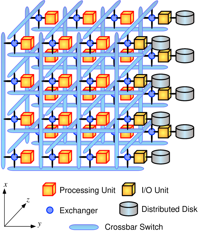
Figure 1: A schematic diagram of the CP-PACS computer.

It is well known that ordinary microprocessors cannot achieve high performance in large scientific/engineering applications because cache memory does not work effectively. In order to solve the problem of long memory access latency which becomes manifest in these applications, the processor of CP-PACS is enhanced by a feature called PVP-SW (pseudo-vector processing based on slide windowed registers) [11]. This feature consists of: (i) a large number of floating point registers (128 in the actual implementation), (ii) two new instructions which request data preloading/poststoring to/from these registers, and (iii) pipelined access to main memory. Long memory access latency can be hidden by issuing data preload instructions well in advance of data usage. Multiple data preloading operations are executed in a pipelined way. The floating point registers are addressed with the slide window mechanism so that the enhancement has upward compatibility with the PA-RISC 1.1 architecture which is taken as the base architecture of the CP-PACS processor.

The hyper-crossbar network has the advantage that it allows data transfer from a node to any other node in at most three steps, and that the system can be divided into independent subsystems easily. Internode communication is enhanced by a feature named remote DMA that executes direct transfer of data between user memory spaces of communicating nodes without using time-consuming system calls. This feature supports the transfer of block-strided data (blocks of continuous data separated by a constant stride) as well as continuous data.

The operating system of CP-PACS is UNIX. Each PU has a micro kernel based on Mach 3.0 and the IOU’s have UNIX servers. The programming languages are Fortran 90, C, C++ and assembler.

The loop-code optimization technique of the compiler is based on a software pipelining technique[11]. Since a sliding of the window changes all the register numbers simultaneously, register allocation can be resolved flexibly. This property makes the optimization technique simple and effective.

We refer to [12] for further details of the architecture of the CP-PACS and its basic performances.

3 Coding lattice QCD on CP-PACS

The basic dynamical variables of QCD are the gluon field and the quark field. On a 4-dimensional lattice of a size $N_{x}\times N_{y}\times N_{z}\times N_{t}$, the gluon field is represented by a set of complex $3\times 3$ matrices $U(n,\mu)$ where $n=(n_{x},n_{y},n_{z},n_{t})$ denotes lattice sites with $1\leq n_{x,y,z,t}\leq N_{x,y,z,t}$ and $\mu=x,y,z,t$ the four directions. The quark field in the Wilson’s formalism is represented by a 12-component complex vector $Q(n)$. The objective of lattice QCD simulations is to numerically evaluate by a Monte Carlo method the Feynman path integral

$$\langle{\cal O}\rangle=\frac{\int{\cal O}(\bar{Q},Q,U)e^{-S(\bar{Q},Q,U)}\prod_{n}d\bar{Q}(n)dQ(n)\prod_{n,\mu}dU(n,\mu)}{\int e^{-S(\bar{Q},Q,U)}\prod_{n}d\bar{Q}(n)dQ(n)\prod_{n,\mu}dU(n,\mu)}$$ (1)

where ${\cal O}(\bar{Q},Q,U)$ is a physical observable and $S(\bar{Q},Q,U)$ the action of lattice QCD describing the interaction of quarks and gluons. Typically the main simulation steps consist of the following:

• 1. Update of the gluon configuration $\{U(n,\mu)\}$ to generate the distribution $e^{-S}$.

  2. Gauge fixing to reduce statistical noise in the measurement of observables.

  3. Solver to compute the quark propagator $G=D^{-1}(U)\,B$ for a number of given quark sources $B$, where the quark matrix $D(U)$ is a sparse $12V\times 12V$ complex matrix depending on the gluon configuration and $V=N_{x}\cdot N_{y}\cdot N_{z}\cdot N_{t}$.

  4. Measurement of hadron observables by combining quark propagators.

The whole cycle is repeated several hundred to several thousand times. The algorithm for the update part differs significantly between quenched simulations, in which the back reaction of quark fields on the distribution of gluon fields is ignored, and full QCD simulations without such an approximation. For full QCD, the most time-consuming computation in the update part is the same as that in the solver part: $G=D^{-1}(U)\,B$. For both cases the computer time is mostly spent in the update part and the solver part, with the update part weighted dominantly for full QCD simulations.

Our performance evaluation data come from a quenched simulation using the entire 2048 PU’s of the CP-PACS, and from a full QCD simulation using a sub-partition consisting of 512 PU’s.

For the quenched simulation, the update part is carried out with the heat-bath [13] and the over-relaxation [14] algorithms mixed in a ratio of 1:4. For the full QCD simulation we adopt the hybrid Monte Carlo algorithm [15].

The computation of $G=D^{-1}(U)\,B$ is performed with a minimal residual algorithm or a BiCGStab algorithm [16]. In the both cases, even-odd preconditioning can be applied. For the quenched simulation we adopt the former, while for full QCD mostly the latter.

Our QCD codes for the CP-PACS are originally developed in FORTRAN90. Let ${\tt Ndimx}\times{\tt Ndimy}\times{\tt Ndimz}$ be the 3-dimensional PU array. We divide the total lattice into ${\tt Ndimx}\times{\tt Ndimy}\times{\tt Ndimz}$ sublattices, each with a size $L_{x}\times L_{y}\times L_{z}\times N_{t}$ with $L_{x}=N_{x}/{\tt Ndimx}$ etc. On each PU the gluon field is then defined as

$${\tt complex\!*\!16}\,\,\,{\tt U(3,3,0:}N_{t}{\tt+1,0:}L_{z}{\tt+1,0:}L_{y}{\tt+1,0:}L_{x}{\tt+1,4)},$$ (2)

for the case of the standard one plaquette gauge action, and

$${\tt complex\!*\!16}\,\,\,{\tt U(3,3,-1:}N_{t}{\tt+2,-1:}L_{z}{\tt+2,-1:}L_{y}{\tt+2,-1:}L_{x}{\tt+2,4)},$$ (3)

for the case of the improved gauge action [17] we adopted in full QCD simulations. For the quark field (or quark propagator to be precise) we introduce

$${\tt complex\!*\!16}\,\,\,{\tt G(3,4,0:}N_{t}{\tt+1,0:}L_{z}{\tt+1,0:}L_{y}{\tt+1,0:}L_{x}{\tt+1)}.$$ (4)

These arrays contain boundaries (ix $\leq 0$ and $\geq L_{x}+1$, etc.), which are the copies of the corresponding variables on the neighboring PU’s. After each modification of U or G, the boundary values have to be renewed. The library functions for a block-strided remote DMA transfer enable us to perform the necessary boundary copies efficiently without gather/scatter manipulations.

A characteristic feature of computations in QCD is that the number of load/store operations, multiplications, and additions are approximately the same. For the heat-bath and over-relaxation updates in quenched QCD, for example, the dominant computation is a matrix multiplication of two gluon variables of form U*U with the two U’s on neighboring links. For each column of the resulting matrix, this computation requires 24 loads, 6 stores, 36 multiplications and 30 additions. The superscalar feature of the CP-PACS processor includes a simultaneous multiplication-addition instruction which can be issued concurrently with a preload/poststore operation. A poststore operation requires two machine cycles on the CP-PACS. Thus computations of the above type can be effectively carried out. The PVP-SW feature solves the remaining problem of large memory access latency and the necessity of a large number of registers to handle a large number of data per loop index. Our compiler can schedule instructions for these loops well. With an appropriate choice of loop unrolling, the FORTRAN code achieves over 160 MFLOPS/PU for the loop, which is over 50% of peak speed.

In the the computation of $G=D^{-1}(U)\,B$ with an iterative algorithm such as minimal residual and BiCGStab, the dominant computation is executed in a subroutine called mult which computes G$\to$D(U)*G. A main part of the calculation, which may be schematically written as V=U*(G₁+G₂), is well balanced requiring 30 loads, 6 stores, 36 multiplications and 36 additions. The remaining computation is less balanced. An efficient scheduling of all these instructions is a fairly complicated task, which the present compiler can cope with only to a modest degree (see Fig. 2). Since an efficient solver is a very important ingredient of lattice QCD simulations, we have written this part of the code in the assembly language [18]. All the instructions are hand-optimized within two long loops paying attention to remove unnecessary load/store operations using the PVP-SW feature. The performance of the assembler code exceeds 190 MFLOPS/PU as shown in Fig. 2.

We emphasize that the loop length for half the peak performance is quite short for our processor, especially for the assembler code. This feature, originating from the pseudo-vectorization on a RISC processor by the software pipelining technique, is in a marked contrast with vector computers; they generally require a long loop length for peak performance, which is usually realized by a one-dimensional addressing of the multi-dimensional coordinate $n$. In our case, we use only the $t$-coordinate for pseudo-vectorization. This made the program quite easy to read and debug.

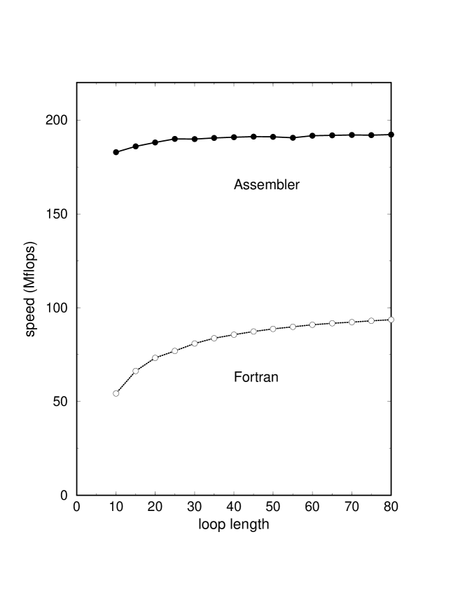
Figure 2: Performance/PU of the core subroutine mult of the solver part with assembler coding as a function of loop length. In our QCD code, the loop length is $N_{t}/2$ due to an even-odd algorithm. The peak speed of a PU is 300 MFLOPSwhen the numbers of multiplications, additions, and loads/stores are equal. Because of an imbalance of these numbers, the theoretical peak speed of this loop is 266 MFLOPS. For comparison, we also plot performance of our fastest FORTRAN code for the same calculation.

Table 2: Execution time of a single cycle of a quenched QCD simulation to study hadron spectroscopy. The lattice size is $64^{3}\times 112$. For the update part, we performed 4 OR sweeps every one HB update. Quark propagators for five different quark masses are solved at the solver part, and the results stored on distributed disks are collected in the measurement part to combine hadron observables.

	execution time (hour)	fraction (%)
update	4.8	30
heat-bath	(1.6)	(10)
over-relaxation	(3.0)	(19)
gauge-fixing	1.3	8
solver	6.8	43
measurement	2.9	19
total	15.7	100

4 Performance of quenched simulation

We now describe the performance of our QCD programs on the CP-PACS computer obtained in our production run for a quenched QCD hadron spectrum calculation with the full 2048 processing units. The lattice size is $64^{3}\times 112$ which is the largest lattice employed so far in lattice QCD simulations. In Table 2 we list a breakdown of the execution time of one cycle of simulation into those of the four basic steps. During the run we measure the execution times of important subroutines using a FORTRAN-supplied interval timer xclock which has the precision of micro seconds. Performance data reported below is based on this measurement averaged over 20 cycles.

Table 3: Profile of the solver program running on the CP-PACS with 2048 PU. The subroutines rbmr and mult are coded in assembler. rbmr is the main routine excluding the subroutine mult, and copyG and gsum executes data transfer and global sum, respectively. The number of floating point operations in gsum is negligible and is ignored.

subroutine	time/call (sec)	#flop	MFLOPS/PU	ratio of exec.time
rbmr	0.0163	3096576	189.8	0.120
mult	0.0482	9289728	192.5	0.707
copyG	0.0098	0	0	0.144
gsum	0.0020	0	0	0.029
solver in total			158.8

4.1 Update of gluon configuration

In quenched QCD simulations, the performance of a gluon update program is often compared in terms of the “link update time”, i.e., the execution time needed to update a single gluon field $U(n,\mu)$ on a link $(n,\mu)$.

The link update time may be translated into GFLOPS using the number of floating operations per link. For the heat bath update, this number cannot be fixed uniquely since the heat bath is a stochastic process and elementary functions are called in the program. We adopt the number 5700 which is widely accepted in the lattice community and has been used in previous estimations[19].

The previous best performance among published data was obtained by the NAL-Yamagata collaboration[19]. Employing the Numerical Wind Tunnel (NWT) with 128 nodes at National Aerospace Laboratory (NAL), they reported a link update time of 0.0317 $\mu$sec or 179.8 GFLOPS, which won the Gordon Bell Prize of 1995. A better performance is listed on the web page of NAL[20]: 215.8 GFLOPS obtained on the enhanced NWT with 160 nodes, corresponding to the link-update time 0.0264 $\mu$sec. Performance on other computers is summarized in [19].

The link update time on the CP-PACS is 0.0240 $\mu$sec. This is equivalent to 237.5 GFLOPS, which exceeds the best value on NWT by 10%.

For the over-relaxation update, our link-update time is 0.0112 $\mu$sec. The number of floating point operations per link can be counted precisely for this case, which equals 3050 using the algorithm we adopted [14]. Therefore, our over-relaxation code achieves 264.6 GFLOPS.

Table 4: Solver performance in the literature

Reported performance data
Machine	VPP500	CM-5	Paragon	T3D	CM-5	ACPMAPS
	(Fujitsu)	(TMC)	(Intel)	(Cray)	(TMC)
location	KEKa	LANLb	—	PSCc	—	Fermilabd
#node	64	—	64	64	64	128
Problem	KS	Wilson	KS	KS	KS	Wilson
MFLOPS/node	1105	35	23.2	22.2	20.0	8.5
GFLOPS	70.7	—	1.5	1.4	1.3	1.1
comment	(1)	(2)	(3)	(3)	(3)	(3)
reference	[21]	[22]	[23]	[23]	[23]	[24]
Possible performance
Machine	NWT	CM-5	Paragon	T3D	CM-5	ACPMAPS
location	NALe	LANLb	SNLf	US Gov.	LANLb	Fermilabd
#node	167	1056	3680	1024	1056	612
GFLOPS	196.1	37.0	85.4	22.7	21.1	5.2
(a) KEK: National Laboratory for High Energy Physics, Japan.
(b) LANL: Los Alamos National Laboratory, USA
(c) PSC: Pittsburgh Supercomputing Center, USA
(d) Fermilab: Fermi National Accelerator Laboratory, USA
(e) NAL: National Aerospace Laboratory, Japan
(f) SNL: Sandia National Laboratories, USA
(1) performance of the core part (mult) of the solver
(2) performance including I/O and setup overhead, MR4 algorithm
(3) conjugate gradient algorithm

4.2 Quark propagator solver

The calculation of performance for the quark propagator solver is made as follows. The computations in the main loop consist of four subroutines (see Table 3). For each subroutine, we measure the execution time per one subroutine call and the ratio of time spent for the subroutine in the total execution time. Counting the number of floating point operations in each subroutine, which can be done precisely, we convert the time data into GFLOPS. The raw data for each subroutine are summarized in Table 3. The average of the performances with weight of the time ratio leads to 158.8 MFLOPS/PU for the solver as a whole, or equivalently 325.3 GFLOPS for the entire CP-PACS system.

For comparison, we reproduce in the top half of Table 4 the performance data for several machines reported in the literature. They refer to either the Wilson quark action used in our run or the Kogut-Susskind quark action which is another form of lattice quark action often used in lattice QCD simulations. The algorithm for the solver also differs as noted in the comments. We should remark in particular that these results are mostly calculated by employing a smaller number of nodes than maximally available. Therefore, we have tried to estimate “possible performance” by assuming that the measured performance scales linearly with the number of nodes up to the maximal configuration with the same architecture which exists now or has existed in the past. This estimate is shown on the bottom half of Table 4.

The best performance for a quark matrix solver recorded has been obtained on the VPP500 with 64 nodes for a KS quark propagator solver. If the reported value is translated to the possible performance on the NWT with 167 nodes, we obtain 196.1 GFLOPS, although NWT has not been used for hadron spectroscopy calculations. The measured performance of 325.3 GFLOPS on the CP-PACS is 66% larger than this.

5 Full QCD simulations

In full QCD simulations, the most time-consuming part is mult both in update and solver. The performance of mult has already been discussed in Sec. 4.2. Here, however, several additional remarks are in order.

First, full QCD simulations are extremely computer-time consuming compared to those of quenched QCD. Simple scaling estimates place a hundred-fold or more increase in the amount of computations for full QCD compared to that of quenched QCD with current algorithms. Therefore, the use of a large lattice comparable to the quenched case is difficult; we are forced to employ coarse lattices.

In order to keep a reasonable sublattice size for each PU, we perform calculations on partitions of the CP-PACS. The largest partition we have used in our full QCD simulation consists of 512 PU’s with a lattice size of $24^{3}\times 48$. We report the performance measured on this lattice. In this case, the vector length is 24 for major loops.

Furthermore, in order to suppress discretization errors caused by the coarse lattice used in full QCD calculations, we apply action improvement which has been widely pursued in the last few years. Based on a comparative study of various combinations of improved and unimproved actions in full QCD [8], we adopt an improved gluon action proposed by Iwasaki [17], combined with an improved quark action suggested by Sheikholeslami and Wohlert [25]. Although the basic structure of the computations can be maintained, improvement of the action implies several additional computations which are coded in FORTRAN in our programs. Together with the short vector length, the relative weight of the FORTRAN parts over the parts coded in the assembly language (such as mult) is much larger than that in the quenched simulations.

In the hybrid Monte Carlo algorithm [15] adopted in our full QCD update, one unit of update calculation is called “trajectory”. Several trajectories are required to suppress autocorrelation among succeeding configurations. In our simulations, we separated the measurement steps by five trajectories.

Major parts of the computer time for one trajectory of full QCD update can be assembled as

$$\left[A_{\rm comp}+A_{\rm commun}+(B_{\rm comp}+B_{\rm commun})\times N_{\rm inv}\right]\times{1\over\Delta\tau}+C,$$ (5)

with negligible $C$. Here, $N_{\rm inv}$ is the number of iteration steps required in the computation of $G=D^{-1}(U)\,B$, and $\Delta\tau$ is the evolution step size for the hybrid Monte Carlo algorithm. In our simulations, $N_{\rm inv}\approx 60$–500 and $1/\Delta\tau\approx 50$–150 depending on the values of physical parameters such as quark mass and lattice volume.

$A_{\rm comp}$ and $B_{\rm comp}$ are contributions from the computations in each PU, whose most time-consuming part is mult. For the case of the algorithm we adopt, we find that the total number of floating point operations for $A_{\rm comp}$ and $B_{\rm comp}$ are $456,000\times V$ and $8,800\times V$, respectively, where $V=N_{x}\times N_{y}\times N_{z}\times N_{t}$ is the lattice volume. Relatively large number of operations for $A_{\rm comp}$ and $B_{\rm comp}$ is due to the improved action and the improved algorithm we use. The speed of $A_{\rm comp}$ and $B_{\rm comp}$ are measured to be 94 and 113 MFLOPS/PU, respectively, which correspond to 31 and 38% of the peak performance.

$A_{\rm commun}$ and $B_{\rm commun}$ are from internode communications. In our simulations, the computer time for $A_{\rm commun}$ is negligible and that for $B_{\rm commun}$ is about 8–10% of $B_{\rm comp}$. Measured throughput for the $B_{\rm commun}$ part was 157 MB/sec on a $24^{3}\times 48$ lattice simulated with a 512 PU partition. An extrapolation to the limit of large $N_{t}$ leads to 192 MB/sec.

6 Summary

We have presented the performance data of the CP-PACS computer measured during recent production runs for Quantum Chromodynamics simulations of quarks and gluons. In a run with the quenched approximation, we used the full 2048 processing nodes of the CP-PACS and obtained a sustained speed of 237.5 GFLOPS for the heat-bath update of gluon variables, 264.6 GFLOPS for the over-relaxation update, and 325.3 GFLOPS for quark matrix inversion with an even-odd preconditioned minimal residual algorithm. These performances correspond to 43–53% of the theoretical peak speed of the CP-PACS. In more recent full QCD simulations in which the quenched approximation is removed, we used sub-partitions of the CP-PACS up to 512 processing nodes. We found 113 MFLOPS/PU for the kernel part of the simulation, which corresponds to 38% of the peak performance.

References

- [1] K.G. Wilson, Phys. Rev. D10 (1974) 2445.
- [2] For introduction to lattice gauge theories, see, M. Creutz, Quarks, Gluons and Lattices (Cambridge University Press, Cambridge, 1988); I. Montvay and G. Münster, Field Theory on the Lattice (Cambridge University Press, Cambridge, 1993).
- [3] For a recent estimation of computer time, see S. Sharpe, hep-lat/9811006, to be published in Proc. of XXIX International Conference on High Energy Physics, Vancouver, Canada, July 23-29 1998.
- [4] For reviews, see, e.g., Y. Iwasaki, Nucl. Phys. B (Proc.Suppl.) 34 (1994) 78; J.C. Sexton, ibid. 47 (1996) 236; and references cited therein.
- [5] The CP-PACS Project has been described in Y. Iwasaki, Nucl. Phys. B (Proc.Suppl.) 60A (1998) 246. See also Y. Iwasaki, ibid. 34 (1994) 78; A. Ukawa, ibid. 42 (1995) 194; Y. Iwasaki, ibid. 53 (1997) 1007. For further details, see, http://www.rccp.tsukuba.ac.jp. The present members of the CP-PACS project are: S. Aoki, R. Burkhalter, T. Boku, M. Fukugita, S. Gunji, T. Hoshino, S. Ichii, M. Imada, N. Ishizuka, Y. Iwasaki, K. Kanaya, H. Kawai, T. Kawai, M. Miyama, S. Miyashita, M. Mori, Y. Nakamoto, H. Nakamura, T. Nakamura, I. Nakata, K. Nakazawa, K. Nemoto, M. Okawa, A. Oshiyama, Y. Oyanagi, S. Sakai, T. Shirakawa, A. Ukawa, M. Umemura, K. Wada, Y. Watase, Y. Yamashita, M. Yasunaga, and T. Yoshié.
- [6] For recent status of other dedicated computer projects in lattice QCD, see A. Baltoloni et al., Nucl. Phys. B (Proc.Suppl.) 63 (1998) 991, and D. Chen et al., ibid. 997.
- [7] CP-PACS Collaboration, S. Aoki et al., Nucl. Phys. B (Proc. Suppl.) 60A (1998) 14; ibid. 63 (1998) 161; hep-lat/9809146, 9810043, to be published in Proceedings of International Workshop on Lattice Field Theories (LATTICE 98), Boulder, CO, July 13-18, 1998 [Nucl. Phys. B (Proc. Suppl.) (1999)].
- [8] CP-PACS Collaboration: S. Aoki et al., hep-lat/9902018. See also Nucl. Phys. B (Proc. Suppl.) 60A (1998) 335; ibid. 63 (1998) 221.
- [9] CP-PACS Collaboration, S. Aoki et al., hep-lat/9809118, 9809120, 9809185, 9810043, to be published in Proceedings of International Workshop on Lattice Field Theories (LATTICE 98), Boulder, CO, July 13-18, 1998 [Nucl. Phys. B (Proc. Suppl.) (1999)].
- [10] A. Ukawa, in this volume.
- [11] H. Nakamura et al., Proc. of ACM International Conference on Supercomputing ’93 (1993) 298; H. Nakamura et al., Proc. of IEEE 27th Hawaii International Conference on System Sciences (1994) 368.
- [12] T. Boku, K. Itakura, H. Nakamura, and K. Nakazawa, “CP-PACS: A massively parallel processor for large scale scientific calculations”, in Proc. International Conference on Supercomputing ’97, pp.108-115.
- [13] N. Cabibbo and E. Marinari, Phys. Lett. B119 (1982) 387; M. Okawa, Phys. Rev. Lett. 49 (1982) 353.
- [14] F.R. Brown and T.J. Woch, Phys. Rev. Lett. 58 (1987) 2397.
- [15] S. Duane, A.D. Kennedy, B.J. Pendleton and D. Roweth, Phys. Lett. B195 (1987) 216; S. Gottlieb, W. Liu, D. Toussaint, R.L. Renken and R.L. Sugar, Phys. Rev. D35 (1987) 2531.
- [16] H. van der Vorst, SIAM J. Sc. Stat. Comp. 13 (1992) 631; A. Frommer, V. Hannemann, B. Nockel, T. Lippert and K. Schilling, Int. J. Mod. Phys. C5 (1994) 1073.
- [17] Y. Iwasaki, Nucl. Phys. B258 (1985) 141; Univ. of Tsukuba report UTHEP-118 (1983), unpublished.
- [18] T. Yoshié, Prog. Theor. Phys. Suppl. 122 (1996) 17.
- [19] M. Yoshida, A. Nakamura, M. Fukuda, T. Nakamura, and S. Hioki, in Proc. 1995 ACM-IEEE Supercomputing, San Diego, 1995, CD-ROM.
- [20] http://www.nal.go.jp/www-e/facility/ns2/home.html
- [21] M. Okawa, Prog. Theor. Phys. Suppl. 122 (1996) 25.
- [22] T. Bhattacharya and R. Gupta, Nucl. Phys. B (Proc. Suppl.) 34 (1994) 341.
- [23] D. Toussaint and R. Sugar, in “1994 Parallel Application Technology Program Research Review”, Pittsburgh Supercomputing Center, http://www.psc.edu/research/parallel_apps/review/toussaint_sugar.html
- [24] M. Fischler and M. Uchima, Nucl. Phys. B (Proc. Suppl.) 47 (1996) 808.
- [25] B. Sheikholeslami and R. Wohlert, Nucl. Phys. B259 (1985) 572.