CERN–EP/99–07

Abstract

• A measurement of the forward–backward asymmetry of $e^{+}e^{-}\to c\bar{c}$ and $e^{+}e^{-}\to b\bar{b}$ on the $Z$ resonance is performed using about 3.5 million hadronic $Z$ decays collected by the DELPHI detector at LEP in the years 1992 to 1995. The heavy quark is tagged by the exclusive reconstruction of several $D$ meson decay modes. The forward–backward asymmetries for $c$ and $b$ quarks at the $Z$ resonance are determined to be:

  $$\begin{array}[]{rcr@{\!\!\;\,}l}{A_{FB}^{c}}(\sqrt{s}=91.235\,{\rm GeV})&=&&0.0659\,\,\pm\,\,0.0094\,(stat)\,\,\pm\,\,0.0035\,(syst)\\ {A_{FB}^{b}}(\sqrt{s}=91.235\,{\rm GeV})&=&&0.0762\,\,\pm\,\,0.0194\,(stat)\,\,\pm\,\,0.0085\,(syst)\\ {A_{FB}^{c}}(\sqrt{s}=89.434\,{\rm GeV})&=&-&0.0496\,\,\pm\,\,0.0368\,(stat)\,\,\pm\,\,0.0053\,(syst)\\ {A_{FB}^{b}}(\sqrt{s}=89.434\,{\rm GeV})&=&&0.0567\,\,\pm\,\,0.0756\,(stat)\,\,\pm\,\,0.0117\,(syst)\\ {A_{FB}^{c}}(\sqrt{s}=92.990\,{\rm GeV})&=&&0.1180\,\,\pm\,\,0.0318\,(stat)\,\,\pm\,\,0.0062\,(syst)\\ {A_{FB}^{b}}(\sqrt{s}=92.990\,{\rm GeV})&=&&0.0882\,\,\pm\,\,0.0633\,(stat)\,\,\pm\,\,0.0122\,(syst)\\ \end{array}$$

  The combination of these results leads to an effective electroweak mixing angle of:

  $${\sin^{2}\theta_{eff}^{lept}}=0.2332\pm 0.0016$$

  (Submitted to Eur. Phys. J. C)

  P.Abreu${}^{\ref{LIP}}$, T.Adye${}^{\ref{RAL}}$, P.Adzic${}^{\ref{DEMOKRITOS}}$, Z.Albrecht${}^{\ref{KARLSRUHE}}$, T.Alderweireld${}^{\ref{AIM}}$, G.D.Alekseev${}^{\ref{JINR}}$, R.Alemany${}^{\ref{VALENCIA}}$, T.Allmendinger${}^{\ref{KARLSRUHE}}$, P.P.Allport${}^{\ref{LIVERPOOL}}$, S.Almehed${}^{\ref{LUND}}$, U.Amaldi${}^{\ref{CERN}}$, S.Amato${}^{\ref{UFRJ}}$, E.G.Anassontzis${}^{\ref{ATHENS}}$, P.Andersson${}^{\ref{STOCKHOLM}}$, A.Andreazza${}^{\ref{CERN}}$, S.Andringa${}^{\ref{LIP}}$, P.Antilogus${}^{\ref{LYON}}$, W-D.Apel${}^{\ref{KARLSRUHE}}$, Y.Arnoud${}^{\ref{CERN}}$, B.Åsman${}^{\ref{STOCKHOLM}}$, J-E.Augustin${}^{\ref{LYON}}$, A.Augustinus${}^{\ref{CERN}}$, P.Baillon${}^{\ref{CERN}}$, P.Bambade${}^{\ref{LAL}}$, F.Barao${}^{\ref{LIP}}$, G.Barbiellini${}^{\ref{TU}}$, R.Barbier${}^{\ref{LYON}}$, D.Y.Bardin${}^{\ref{JINR}}$, G.Barker${}^{\ref{KARLSRUHE}}$, A.Baroncelli${}^{\ref{ROMA3}}$, M.Battaglia${}^{\ref{HELSINKI}}$, M.Baubillier${}^{\ref{LPNHE}}$, K-H.Becks${}^{\ref{WUPPERTAL}}$, M.Begalli${}^{\ref{BRASIL}}$, P.Beilliere${}^{\ref{CDF}}$, Yu.Belokopytov${}^{\ref{CERN},\ref{MILAN-SERPOU}}$, K.Belous${}^{\ref{SERPUKHOV}}$, A.C.Benvenuti${}^{\ref{BOLOGNA}}$, C.Berat${}^{\ref{GRENOBLE}}$, M.Berggren${}^{\ref{LYON}}$, D.Bertini${}^{\ref{LYON}}$, D.Bertrand${}^{\ref{AIM}}$, M.Besancon${}^{\ref{SACLAY}}$, F.Bianchi${}^{\ref{TORINO}}$, M.Bigi${}^{\ref{TORINO}}$, M.S.Bilenky${}^{\ref{JINR}}$, M-A.Bizouard${}^{\ref{LAL}}$, D.Bloch${}^{\ref{CRN}}$, H.M.Blom${}^{\ref{NIKHEF}}$, M.Bonesini${}^{\ref{MILANO}}$, W.Bonivento${}^{\ref{MILANO}}$, M.Boonekamp${}^{\ref{SACLAY}}$, P.S.L.Booth${}^{\ref{LIVERPOOL}}$, A.W.Borgland${}^{\ref{BERGEN}}$, G.Borisov${}^{\ref{LAL}}$, C.Bosio${}^{\ref{SAPIENZA}}$, O.Botner${}^{\ref{UPPSALA}}$, E.Boudinov${}^{\ref{NIKHEF}}$, B.Bouquet${}^{\ref{LAL}}$, C.Bourdarios${}^{\ref{LAL}}$, T.J.V.Bowcock${}^{\ref{LIVERPOOL}}$, I.Boyko${}^{\ref{JINR}}$, I.Bozovic${}^{\ref{DEMOKRITOS}}$, M.Bozzo${}^{\ref{GENOVA}}$, P.Branchini${}^{\ref{ROMA3}}$, T.Brenke${}^{\ref{WUPPERTAL}}$, R.A.Brenner${}^{\ref{UPPSALA}}$, P.Bruckman${}^{\ref{KRAKOW}}$, J-M.Brunet${}^{\ref{CDF}}$, L.Bugge${}^{\ref{OSLO}}$, T.Buran${}^{\ref{OSLO}}$, T.Burgsmueller${}^{\ref{WUPPERTAL}}$, P.Buschmann${}^{\ref{WUPPERTAL}}$, S.Cabrera${}^{\ref{VALENCIA}}$, M.Caccia${}^{\ref{MILANO}}$, M.Calvi${}^{\ref{MILANO}}$, T.Camporesi${}^{\ref{CERN}}$, V.Canale${}^{\ref{ROMA2}}$, F.Carena${}^{\ref{CERN}}$, L.Carroll${}^{\ref{LIVERPOOL}}$, C.Caso${}^{\ref{GENOVA}}$, M.V.Castillo Gimenez${}^{\ref{VALENCIA}}$, A.Cattai${}^{\ref{CERN}}$, F.R.Cavallo${}^{\ref{BOLOGNA}}$, V.Chabaud${}^{\ref{CERN}}$, M.Chapkin${}^{\ref{SERPUKHOV}}$, Ph.Charpentier${}^{\ref{CERN}}$, L.Chaussard${}^{\ref{LYON}}$, P.Checchia${}^{\ref{PADOVA}}$, G.A.Chelkov${}^{\ref{JINR}}$, R.Chierici${}^{\ref{TORINO}}$, P.Chliapnikov${}^{\ref{SERPUKHOV}}$, P.Chochula${}^{\ref{BRATISLAVA}}$, V.Chorowicz${}^{\ref{LYON}}$, J.Chudoba${}^{\ref{NC}}$, K.Cieslik${}^{\ref{KRAKOW}}$, P.Collins${}^{\ref{CERN}}$, R.Contri${}^{\ref{GENOVA}}$, E.Cortina${}^{\ref{VALENCIA}}$, G.Cosme${}^{\ref{LAL}}$, F.Cossutti${}^{\ref{CERN}}$, J-H.Cowell${}^{\ref{LIVERPOOL}}$, H.B.Crawley${}^{\ref{AMES}}$, D.Crennell${}^{\ref{RAL}}$, S.Crepe${}^{\ref{GRENOBLE}}$, G.Crosetti${}^{\ref{GENOVA}}$, J.Cuevas Maestro${}^{\ref{OVIEDO}}$, S.Czellar${}^{\ref{HELSINKI}}$, M.Davenport${}^{\ref{CERN}}$, W.Da Silva${}^{\ref{LPNHE}}$, A.Deghorain${}^{\ref{AIM}}$, G.Della Ricca${}^{\ref{TU}}$, P.Delpierre${}^{\ref{MARSEILLE}}$, N.Demaria${}^{\ref{CERN}}$, A.De Angelis${}^{\ref{CERN}}$, W.De Boer${}^{\ref{KARLSRUHE}}$, S.De Brabandere${}^{\ref{AIM}}$, C.De Clercq${}^{\ref{AIM}}$, B.De Lotto${}^{\ref{TU}}$, A.De Min${}^{\ref{PADOVA}}$, L.De Paula${}^{\ref{UFRJ}}$, H.Dijkstra${}^{\ref{CERN}}$, L.Di Ciaccio${}^{\ref{ROMA2},\ref{CERN}}$, J.Dolbeau${}^{\ref{CDF}}$, K.Doroba${}^{\ref{WARSZAWA}}$, M.Dracos${}^{\ref{CRN}}$, J.Drees${}^{\ref{WUPPERTAL}}$, M.Dris${}^{\ref{NTU-ATHENS}}$, A.Duperrin${}^{\ref{LYON}}$, J-D.Durand${}^{\ref{CERN}}$, G.Eigen${}^{\ref{BERGEN}}$, T.Ekelof${}^{\ref{UPPSALA}}$, G.Ekspong${}^{\ref{STOCKHOLM}}$, M.Ellert${}^{\ref{UPPSALA}}$, M.Elsing${}^{\ref{CERN}}$, J-P.Engel${}^{\ref{CRN}}$, B.Erzen${}^{\ref{SLOVENIJA}}$, M.Espirito Santo${}^{\ref{LIP}}$, E.Falk${}^{\ref{LUND}}$, G.Fanourakis${}^{\ref{DEMOKRITOS}}$, D.Fassouliotis${}^{\ref{DEMOKRITOS}}$, J.Fayot${}^{\ref{LPNHE}}$, M.Feindt${}^{\ref{KARLSRUHE}}$, A.Fenyuk${}^{\ref{SERPUKHOV}}$, P.Ferrari${}^{\ref{MILANO}}$, A.Ferrer${}^{\ref{VALENCIA}}$, E.Ferrer-Ribas${}^{\ref{LAL}}$, S.Fichet${}^{\ref{LPNHE}}$, A.Firestone${}^{\ref{AMES}}$, U.Flagmeyer${}^{\ref{WUPPERTAL}}$, H.Foeth${}^{\ref{CERN}}$, E.Fokitis${}^{\ref{NTU-ATHENS}}$, F.Fontanelli${}^{\ref{GENOVA}}$, B.Franek${}^{\ref{RAL}}$, A.G.Frodesen${}^{\ref{BERGEN}}$, R.Fruhwirth${}^{\ref{VIENNA}}$, F.Fulda-Quenzer${}^{\ref{LAL}}$, J.Fuster${}^{\ref{VALENCIA}}$, A.Galloni${}^{\ref{LIVERPOOL}}$, D.Gamba${}^{\ref{TORINO}}$, S.Gamblin${}^{\ref{LAL}}$, M.Gandelman${}^{\ref{UFRJ}}$, C.Garcia${}^{\ref{VALENCIA}}$, C.Gaspar${}^{\ref{CERN}}$, M.Gaspar${}^{\ref{UFRJ}}$, U.Gasparini${}^{\ref{PADOVA}}$, Ph.Gavillet${}^{\ref{CERN}}$, E.N.Gazis${}^{\ref{NTU-ATHENS}}$, D.Gele${}^{\ref{CRN}}$, N.Ghodbane${}^{\ref{LYON}}$, I.Gil${}^{\ref{VALENCIA}}$, F.Glege${}^{\ref{WUPPERTAL}}$, R.Gokieli${}^{\ref{CERN},\ref{WARSZAWA}}$, B.Golob${}^{\ref{SLOVENIJA}}$, G.Gomez-Ceballos${}^{\ref{SANTANDER}}$, P.Goncalves${}^{\ref{LIP}}$, I.Gonzalez Caballero${}^{\ref{SANTANDER}}$, G.Gopal${}^{\ref{RAL}}$, L.Gorn${}^{\ref{AMES},\ref{FLORIDA}}$, M.Gorski${}^{\ref{WARSZAWA}}$, Yu.Gouz${}^{\ref{SERPUKHOV}}$, V.Gracco${}^{\ref{GENOVA}}$, J.Grahl${}^{\ref{AMES}}$, E.Graziani${}^{\ref{ROMA3}}$, C.Green${}^{\ref{LIVERPOOL}}$, H-J.Grimm${}^{\ref{KARLSRUHE}}$, P.Gris${}^{\ref{SACLAY}}$, G.Grosdidier${}^{\ref{LAL}}$, K.Grzelak${}^{\ref{WARSZAWA}}$, M.Gunther${}^{\ref{UPPSALA}}$, J.Guy${}^{\ref{RAL}}$, F.Hahn${}^{\ref{CERN}}$, S.Hahn${}^{\ref{WUPPERTAL}}$, S.Haider${}^{\ref{CERN}}$, A.Hallgren${}^{\ref{UPPSALA}}$, K.Hamacher${}^{\ref{WUPPERTAL}}$, J.Hansen${}^{\ref{OSLO}}$, F.J.Harris${}^{\ref{OXFORD}}$, V.Hedberg${}^{\ref{LUND}}$, S.Heising${}^{\ref{KARLSRUHE}}$, J.J.Hernandez${}^{\ref{VALENCIA}}$, P.Herquet${}^{\ref{AIM}}$, H.Herr${}^{\ref{CERN}}$, T.L.Hessing${}^{\ref{OXFORD}}$, J.-M.Heuser${}^{\ref{WUPPERTAL}}$, E.Higon${}^{\ref{VALENCIA}}$, S-O.Holmgren${}^{\ref{STOCKHOLM}}$, P.J.Holt${}^{\ref{OXFORD}}$, S.Hoorelbeke${}^{\ref{AIM}}$, M.Houlden${}^{\ref{LIVERPOOL}}$, J.Hrubec${}^{\ref{VIENNA}}$, K.Huet${}^{\ref{AIM}}$, G.J.Hughes${}^{\ref{LIVERPOOL}}$, K.Hultqvist${}^{\ref{STOCKHOLM}}$, J.N.Jackson${}^{\ref{LIVERPOOL}}$, R.Jacobsson${}^{\ref{CERN}}$, P.Jalocha${}^{\ref{CERN}}$, R.Janik${}^{\ref{BRATISLAVA}}$, Ch.Jarlskog${}^{\ref{LUND}}$, G.Jarlskog${}^{\ref{LUND}}$, P.Jarry${}^{\ref{SACLAY}}$, B.Jean-Marie${}^{\ref{LAL}}$, E.K.Johansson${}^{\ref{STOCKHOLM}}$, P.Jonsson${}^{\ref{LYON}}$, C.Joram${}^{\ref{CERN}}$, P.Juillot${}^{\ref{CRN}}$, F.Kapusta${}^{\ref{LPNHE}}$, K.Karafasoulis${}^{\ref{DEMOKRITOS}}$, S.Katsanevas${}^{\ref{LYON}}$, E.C.Katsoufis${}^{\ref{NTU-ATHENS}}$, R.Keranen${}^{\ref{KARLSRUHE}}$, B.P.Kersevan${}^{\ref{SLOVENIJA}}$, B.A.Khomenko${}^{\ref{JINR}}$, N.N.Khovanski${}^{\ref{JINR}}$, A.Kiiskinen${}^{\ref{HELSINKI}}$, B.King${}^{\ref{LIVERPOOL}}$, A.Kinvig${}^{\ref{LIVERPOOL}}$, N.J.Kjaer${}^{\ref{NIKHEF}}$, O.Klapp${}^{\ref{WUPPERTAL}}$, H.Klein${}^{\ref{CERN}}$, P.Kluit${}^{\ref{NIKHEF}}$, P.Kokkinias${}^{\ref{DEMOKRITOS}}$, M.Koratzinos${}^{\ref{CERN}}$, V.Kostioukhine${}^{\ref{SERPUKHOV}}$, C.Kourkoumelis${}^{\ref{ATHENS}}$, O.Kouznetsov${}^{\ref{SACLAY}}$, M.Krammer${}^{\ref{VIENNA}}$, E.Kriznic${}^{\ref{SLOVENIJA}}$, P.Krstic${}^{\ref{DEMOKRITOS}}$, Z.Krumstein${}^{\ref{JINR}}$, P.Kubinec${}^{\ref{BRATISLAVA}}$, J.Kurowska${}^{\ref{WARSZAWA}}$, K.Kurvinen${}^{\ref{HELSINKI}}$, J.W.Lamsa${}^{\ref{AMES}}$, D.W.Lane${}^{\ref{AMES}}$, P.Langefeld${}^{\ref{WUPPERTAL}}$, V.Lapin${}^{\ref{SERPUKHOV}}$, J-P.Laugier${}^{\ref{SACLAY}}$, R.Lauhakangas${}^{\ref{HELSINKI}}$, G.Leder${}^{\ref{VIENNA}}$, F.Ledroit${}^{\ref{GRENOBLE}}$, V.Lefebure${}^{\ref{AIM}}$, L.Leinonen${}^{\ref{STOCKHOLM}}$, A.Leisos${}^{\ref{DEMOKRITOS}}$, R.Leitner${}^{\ref{NC}}$, J.Lemonne${}^{\ref{AIM}}$, G.Lenzen${}^{\ref{WUPPERTAL}}$, V.Lepeltier${}^{\ref{LAL}}$, T.Lesiak${}^{\ref{KRAKOW}}$, M.Lethuillier${}^{\ref{SACLAY}}$, J.Libby${}^{\ref{OXFORD}}$, D.Liko${}^{\ref{CERN}}$, A.Lipniacka${}^{\ref{STOCKHOLM}}$, I.Lippi${}^{\ref{PADOVA}}$, B.Loerstad${}^{\ref{LUND}}$, J.G.Loken${}^{\ref{OXFORD}}$, J.H.Lopes${}^{\ref{UFRJ}}$, J.M.Lopez${}^{\ref{SANTANDER}}$, R.Lopez-Fernandez${}^{\ref{GRENOBLE}}$, D.Loukas${}^{\ref{DEMOKRITOS}}$, P.Lutz${}^{\ref{SACLAY}}$, L.Lyons${}^{\ref{OXFORD}}$, J.MacNaughton${}^{\ref{VIENNA}}$, J.R.Mahon${}^{\ref{BRASIL}}$, A.Maio${}^{\ref{LIP}}$, A.Malek${}^{\ref{WUPPERTAL}}$, T.G.M.Malmgren${}^{\ref{STOCKHOLM}}$, V.Malychev${}^{\ref{JINR}}$, F.Mandl${}^{\ref{VIENNA}}$, J.Marco${}^{\ref{SANTANDER}}$, R.Marco${}^{\ref{SANTANDER}}$, B.Marechal${}^{\ref{UFRJ}}$, M.Margoni${}^{\ref{PADOVA}}$, J-C.Marin${}^{\ref{CERN}}$, C.Mariotti${}^{\ref{CERN}}$, A.Markou${}^{\ref{DEMOKRITOS}}$, C.Martinez-Rivero${}^{\ref{LAL}}$, F.Martinez-Vidal${}^{\ref{VALENCIA}}$, S.Marti i Garcia${}^{\ref{CERN}}$, J.Masik${}^{\ref{FZU}}$, N.Mastroyiannopoulos${}^{\ref{DEMOKRITOS}}$, F.Matorras${}^{\ref{SANTANDER}}$, C.Matteuzzi${}^{\ref{MILANO}}$, G.Matthiae${}^{\ref{ROMA2}}$, F.Mazzucato${}^{\ref{PADOVA}}$, M.Mazzucato${}^{\ref{PADOVA}}$, M.Mc Cubbin${}^{\ref{LIVERPOOL}}$, R.Mc Kay${}^{\ref{AMES}}$, R.Mc Nulty${}^{\ref{LIVERPOOL}}$, G.Mc Pherson${}^{\ref{LIVERPOOL}}$, C.Meroni${}^{\ref{MILANO}}$, W.T.Meyer${}^{\ref{AMES}}$, E.Migliore${}^{\ref{TORINO}}$, L.Mirabito${}^{\ref{LYON}}$, W.A.Mitaroff${}^{\ref{VIENNA}}$, U.Mjoernmark${}^{\ref{LUND}}$, T.Moa${}^{\ref{STOCKHOLM}}$, M.Moch${}^{\ref{KARLSRUHE}}$, R.Moeller${}^{\ref{NBI}}$, K.Moenig${}^{\ref{CERN}}$, M.R.Monge${}^{\ref{GENOVA}}$, X.Moreau${}^{\ref{LPNHE}}$, P.Morettini${}^{\ref{GENOVA}}$, G.Morton${}^{\ref{OXFORD}}$, U.Mueller${}^{\ref{WUPPERTAL}}$, K.Muenich${}^{\ref{WUPPERTAL}}$, M.Mulders${}^{\ref{NIKHEF}}$, C.Mulet-Marquis${}^{\ref{GRENOBLE}}$, R.Muresan${}^{\ref{LUND}}$, W.J.Murray${}^{\ref{RAL}}$, B.Muryn${}^{\ref{GRENOBLE},\ref{KRAKOW}}$, G.Myatt${}^{\ref{OXFORD}}$, T.Myklebust${}^{\ref{OSLO}}$, F.Naraghi${}^{\ref{GRENOBLE}}$, F.L.Navarria${}^{\ref{BOLOGNA}}$, S.Navas${}^{\ref{VALENCIA}}$, K.Nawrocki${}^{\ref{WARSZAWA}}$, P.Negri${}^{\ref{MILANO}}$, S.Nemecek${}^{\ref{FZU}}$, N.Neufeld${}^{\ref{CERN}}$, N.Neumeister${}^{\ref{VIENNA}}$, R.Nicolaidou${}^{\ref{SACLAY}}$, B.S.Nielsen${}^{\ref{NBI}}$, M.Nikolenko${}^{\ref{CRN},\ref{JINR}}$, V.Nomokonov${}^{\ref{HELSINKI}}$, A.Normand${}^{\ref{LIVERPOOL}}$, A.Nygren${}^{\ref{LUND}}$, V.Obraztsov${}^{\ref{SERPUKHOV}}$, A.G.Olshevski${}^{\ref{JINR}}$, A.Onofre${}^{\ref{LIP}}$, R.Orava${}^{\ref{HELSINKI}}$, G.Orazi${}^{\ref{CRN}}$, K.Osterberg${}^{\ref{HELSINKI}}$, A.Ouraou${}^{\ref{SACLAY}}$, M.Paganoni${}^{\ref{MILANO}}$, S.Paiano${}^{\ref{BOLOGNA}}$, R.Pain${}^{\ref{LPNHE}}$, R.Paiva${}^{\ref{LIP}}$, J.Palacios${}^{\ref{OXFORD}}$, H.Palka${}^{\ref{KRAKOW}}$, Th.D.Papadopoulou${}^{\ref{NTU-ATHENS}}$, K.Papageorgiou${}^{\ref{DEMOKRITOS}}$, L.Pape${}^{\ref{CERN}}$, C.Parkes${}^{\ref{CERN}}$, F.Parodi${}^{\ref{GENOVA}}$, U.Parzefall${}^{\ref{LIVERPOOL}}$, A.Passeri${}^{\ref{ROMA3}}$, O.Passon${}^{\ref{WUPPERTAL}}$, M.Pegoraro${}^{\ref{PADOVA}}$, L.Peralta${}^{\ref{LIP}}$, M.Pernicka${}^{\ref{VIENNA}}$, A.Perrotta${}^{\ref{BOLOGNA}}$, C.Petridou${}^{\ref{TU}}$, A.Petrolini${}^{\ref{GENOVA}}$, H.T.Phillips${}^{\ref{RAL}}$, F.Pierre${}^{\ref{SACLAY}}$, M.Pimenta${}^{\ref{LIP}}$, E.Piotto${}^{\ref{MILANO}}$, T.Podobnik${}^{\ref{SLOVENIJA}}$, M.E.Pol${}^{\ref{BRASIL}}$, G.Polok${}^{\ref{KRAKOW}}$, P.Poropat${}^{\ref{TU}}$, V.Pozdniakov${}^{\ref{JINR}}$, P.Privitera${}^{\ref{ROMA2}}$, N.Pukhaeva${}^{\ref{JINR}}$, A.Pullia${}^{\ref{MILANO}}$, D.Radojicic${}^{\ref{OXFORD}}$, S.Ragazzi${}^{\ref{MILANO}}$, H.Rahmani${}^{\ref{NTU-ATHENS}}$, D.Rakoczy${}^{\ref{VIENNA}}$, P.N.Ratoff${}^{\ref{LANCASTER}}$, A.L.Read${}^{\ref{OSLO}}$, P.Rebecchi${}^{\ref{CERN}}$, N.G.Redaelli${}^{\ref{MILANO}}$, M.Regler${}^{\ref{VIENNA}}$, D.Reid${}^{\ref{NIKHEF}}$, R.Reinhardt${}^{\ref{WUPPERTAL}}$, P.B.Renton${}^{\ref{OXFORD}}$, L.K.Resvanis${}^{\ref{ATHENS}}$, F.Richard${}^{\ref{LAL}}$, J.Ridky${}^{\ref{FZU}}$, G.Rinaudo${}^{\ref{TORINO}}$, O.Rohne${}^{\ref{OSLO}}$, A.Romero${}^{\ref{TORINO}}$, P.Ronchese${}^{\ref{PADOVA}}$, E.I.Rosenberg${}^{\ref{AMES}}$, P.Rosinsky${}^{\ref{BRATISLAVA}}$, P.Roudeau${}^{\ref{LAL}}$, T.Rovelli${}^{\ref{BOLOGNA}}$, Ch.Royon${}^{\ref{SACLAY}}$, V.Ruhlmann-Kleider${}^{\ref{SACLAY}}$, A.Ruiz${}^{\ref{SANTANDER}}$, H.Saarikko${}^{\ref{HELSINKI}}$, Y.Sacquin${}^{\ref{SACLAY}}$, A.Sadovsky${}^{\ref{JINR}}$, G.Sajot${}^{\ref{GRENOBLE}}$, J.Salt${}^{\ref{VALENCIA}}$, D.Sampsonidis${}^{\ref{DEMOKRITOS}}$, M.Sannino${}^{\ref{GENOVA}}$, H.Schneider${}^{\ref{KARLSRUHE}}$, Ph.Schwemling${}^{\ref{LPNHE}}$, U.Schwickerath${}^{\ref{KARLSRUHE}}$, M.A.E.Schyns${}^{\ref{WUPPERTAL}}$, F.Scuri${}^{\ref{TU}}$, P.Seager${}^{\ref{LANCASTER}}$, Y.Sedykh${}^{\ref{JINR}}$, A.M.Segar${}^{\ref{OXFORD}}$, R.Sekulin${}^{\ref{RAL}}$, R.C.Shellard${}^{\ref{BRASIL}}$, A.Sheridan${}^{\ref{LIVERPOOL}}$, M.Siebel${}^{\ref{WUPPERTAL}}$, L.Simard${}^{\ref{SACLAY}}$, F.Simonetto${}^{\ref{PADOVA}}$, A.N.Sisakian${}^{\ref{JINR}}$, G.Smadja${}^{\ref{LYON}}$, N.Smirnov${}^{\ref{SERPUKHOV}}$, O.Smirnova${}^{\ref{LUND}}$, G.R.Smith${}^{\ref{RAL}}$, A.Sopczak${}^{\ref{KARLSRUHE}}$, R.Sosnowski${}^{\ref{WARSZAWA}}$, T.Spassov${}^{\ref{LIP}}$, E.Spiriti${}^{\ref{ROMA3}}$, P.Sponholz${}^{\ref{WUPPERTAL}}$, S.Squarcia${}^{\ref{GENOVA}}$, D.Stampfer${}^{\ref{VIENNA}}$, C.Stanescu${}^{\ref{ROMA3}}$, S.Stanic${}^{\ref{SLOVENIJA}}$, K.Stevenson${}^{\ref{OXFORD}}$, A.Stocchi${}^{\ref{LAL}}$, J.Strauss${}^{\ref{VIENNA}}$, R.Strub${}^{\ref{CRN}}$, B.Stugu${}^{\ref{BERGEN}}$, M.Szczekowski${}^{\ref{WARSZAWA}}$, M.Szeptycka${}^{\ref{WARSZAWA}}$, T.Tabarelli${}^{\ref{MILANO}}$, F.Tegenfeldt${}^{\ref{UPPSALA}}$, F.Terranova${}^{\ref{MILANO}}$, J.Thomas${}^{\ref{OXFORD}}$, J.Timmermans${}^{\ref{NIKHEF}}$, N.Tinti${}^{\ref{BOLOGNA}}$, L.G.Tkatchev${}^{\ref{JINR}}$, S.Todorova${}^{\ref{CRN}}$, A.Tomaradze${}^{\ref{AIM}}$, B.Tome${}^{\ref{LIP}}$, A.Tonazzo${}^{\ref{CERN}}$, L.Tortora${}^{\ref{ROMA3}}$, G.Transtromer${}^{\ref{LUND}}$, D.Treille${}^{\ref{CERN}}$, G.Tristram${}^{\ref{CDF}}$, M.Trochimczuk${}^{\ref{WARSZAWA}}$, C.Troncon${}^{\ref{MILANO}}$, A.Tsirou${}^{\ref{CERN}}$, M-L.Turluer${}^{\ref{SACLAY}}$, I.A.Tyapkin${}^{\ref{JINR}}$, S.Tzamarias${}^{\ref{DEMOKRITOS}}$, B.Ueberschaer${}^{\ref{WUPPERTAL}}$, O.Ullaland${}^{\ref{CERN}}$, V.Uvarov${}^{\ref{SERPUKHOV}}$, G.Valenti${}^{\ref{BOLOGNA}}$, E.Vallazza${}^{\ref{TU}}$, G.W.Van Apeldoorn${}^{\ref{NIKHEF}}$, P.Van Dam${}^{\ref{NIKHEF}}$, W.K.Van Doninck${}^{\ref{AIM}}$, J.Van Eldik${}^{\ref{NIKHEF}}$, A.Van Lysebetten${}^{\ref{AIM}}$, I.Van Vulpen${}^{\ref{NIKHEF}}$, N.Vassilopoulos${}^{\ref{OXFORD}}$, G.Vegni${}^{\ref{MILANO}}$, L.Ventura${}^{\ref{PADOVA}}$, W.Venus${}^{\ref{RAL},\ref{CERN}}$, F.Verbeure${}^{\ref{AIM}}$, M.Verlato${}^{\ref{PADOVA}}$, L.S.Vertogradov${}^{\ref{JINR}}$, V.Verzi${}^{\ref{ROMA2}}$, D.Vilanova${}^{\ref{SACLAY}}$, L.Vitale${}^{\ref{TU}}$, E.Vlasov${}^{\ref{SERPUKHOV}}$, A.S.Vodopyanov${}^{\ref{JINR}}$, C.Vollmer${}^{\ref{KARLSRUHE}}$, G.Voulgaris${}^{\ref{ATHENS}}$, V.Vrba${}^{\ref{FZU}}$, H.Wahlen${}^{\ref{WUPPERTAL}}$, C.Walck${}^{\ref{STOCKHOLM}}$, C.Weiser${}^{\ref{KARLSRUHE}}$, D.Wicke${}^{\ref{WUPPERTAL}}$, J.H.Wickens${}^{\ref{AIM}}$, G.R.Wilkinson${}^{\ref{CERN}}$, M.Winter${}^{\ref{CRN}}$, M.Witek${}^{\ref{KRAKOW}}$, G.Wolf${}^{\ref{CERN}}$, J.Yi${}^{\ref{AMES}}$, O.Yushchenko${}^{\ref{SERPUKHOV}}$, A.Zaitsev${}^{\ref{SERPUKHOV}}$, A.Zalewska${}^{\ref{KRAKOW}}$, P.Zalewski${}^{\ref{WARSZAWA}}$, D.Zavrtanik${}^{\ref{SLOVENIJA}}$, E.Zevgolatakos${}^{\ref{DEMOKRITOS}}$, N.I.Zimin${}^{\ref{JINR},\ref{LUND}}$, G.C.Zucchelli${}^{\ref{STOCKHOLM}}$, G.Zumerle${}^{\ref{PADOVA}}$

  1 Introduction

  The cross–section for the process $e^{+}e^{-}\to Z\to f\bar{f}$ for the fermion $f$ as a function of its polar angle $\theta$ with respect to the direction of the $e^{-}$ can be expressed as:

  $$\frac{d\sigma}{d\cos\theta}\propto 1+\frac{8}{3}\,{A_{FB}^{f}}\,\cos\theta+\cos^{2}\theta\,.$$

  The term proportional to $\cos\theta$ generates a forward–backward asymmetry $A_{FB}^{f}$which results from the interference of the vector ($v$) and axial vector ($a$) couplings of the initial and final state fermions of the $Z$ boson. The improved Born level asymmetry using the effective couplings for pure $Z$ exchange is given by:

  $${A_{FB}^{f}}=\frac{3}{4}\,\,\frac{2\,\bar{v}_{\rm e}\,\bar{a}_{\rm e}}{\bar{v}^{2}_{\rm e}+\bar{a}^{2}_{\rm e}}\,\,\frac{2\,\bar{v}_{f}\,\bar{a}_{f}}{\bar{v}^{2}_{f}+\bar{a}^{2}_{f}}$$

  The measurement of the forward–backward asymmetry for the different fermions in the final state can thus be used to measure $v/a$, and hence to determine the electroweak mixing angle $\sin^{2}\theta_{eff}^{lept}$.

  In this analysis, the forward–backward asymmetries for the processes $e^{+}e^{-}\rightarrow c\bar{c}$ and $e^{+}e^{-}\rightarrow b\bar{b}$ at the $Z$ resonance are measured using reconstructed $D$ mesons in the modes:
  

  $D^{\ast+}$	$\to$ $D^{0}\pi^{+}$
  	$\to$ $(K^{-}\pi^{+})\pi^{+}$
  	$\to$ $(K^{-}\pi^{+}\pi^{-}\pi^{+})\pi^{+}$
  	$\to$ $(K^{-}\pi^{+}(\pi^{0}))\pi^{+}$		with and without $\pi^{0}$ reconstruction
  	$\to$ $(K^{-}\mu^{+}(\nu_{\mu}))\pi^{+}$
  	$\to$ $(K^{-}e^{+}(\nu_{e}))\pi^{+}$
  $D^{0}$	$\to$ $K^{-}\pi^{+}$
  $D^{0}$	$\to$ $K^{-}\pi^{+}(\pi^{0})$		without $\pi^{0}$ reconstruction
  $D^{+}$	$\to$ $K^{-}\pi^{+}\pi^{+}$

  
  

  The $D$ meson contains a charm quark and therefore provides a clean signature of a $c\bar{c}$ event or a decay of a heavy $b$–hadron in a $b\bar{b}$ event. In both cases the charge state of the $D$ is directly correlated to the charge of the primary quark.

  Particle identification in the DELPHI detector is provided by ring imaging Cherenkov counters (RICH), the specific energy loss $dE/dx$ in the Time Projection Chamber (TPC), and electron and muon identification (see section 2); together with $\pi^{0}$ reconstruction, it is used to identify the $D$ decay products and to reduce the combinatorial background.

  It is necessary to distinguish between the contributions of $D$ mesons from $c$ and $b$ quark events in order to determine the individual forward–backward asymmetries. In this analysis a simultaneous fit is performed in terms of the scaled energy $X_{E}=2E_{D}/\sqrt{s}$ (where $E_{D}$ is the energy of the $D$) and the $b$-tagging probability variable (see section 5). The forward–backward asymmetry is then extracted from the distribution of the cosine of the polar angle of the thrust axis signed by the charge state of the $D$ meson.

  In this paper an update of previous DELPHI results [1] is presented. All LEP 1 data collected by the DELPHI detector in the years 1992 to 1995 are used. The high quality of the data through the final LEP 1 reprocessing in combination with improved reconstruction and $b$-tagging techniques [2] result in a significant gain in statistical precision.

  2 The DELPHI Detector

  The DELPHI detector consists of several independent devices for tracking, calorimetry and lepton and hadron identification. The components relevant for this analysis will be briefly described in the following. A detailed description of the whole apparatus and its performance can be found in [3].

  In the barrel region the innermost component is the vertex detector (VD) near to the LEP beam pipe. The VD consists of three concentric layers (closer, inner and outer) of silicon microstrip detectors. Since 1994 the VD provides $R\phi$ and $z$ information in the closer and outer layer and has an extended polar angle coverage of $25^{\circ}<\theta<155^{\circ}$ (closer layer). For polar angles of $44^{\circ}<\theta<136^{\circ}$, a particle crosses all three layers of the VD. With an intrinsic $R\phi$ resolution of $7.6\,{\rm\mu m}$ [3], the VD is the main component for reconstructing secondary vertices of heavy hadron decays.

  The inner detector (ID) is outside the VD and consisted of a jet-chamber to perform a precise $R\phi$ measurement, and five cylindrical MWPC layers. In 1995 the MWPC layers were replaced by five layers of straw tube detectors.

  The ID is followed by the TPC, the main tracking device in DELPHI. It covers polar angles between $21^{\circ}<\theta<159^{\circ}$ with a single point resolution for charged particles of approximately $250\,\mu$m in $R\phi$ and $880\,\mu$m in $z$ [3]. The analysis of the pulse heights of the signals of up to 192 sense wires allows the determination of the specific energy loss, $dE/dx$, of charged particles which can be used for particle identification (see section 4).

  The barrel ring imaging Cherenkov counter is behind the TPC. Its gas and liquid radiators allow particle identification for pions, kaons and protons over almost the whole momentum range (see section 4).

  The outer detector (OD) is mounted behind the RICH to give additional tracking information. It improves significantly the momentum resolution due to its large distance from the interaction point. Five layers of drift cells cover polar angles between $42^{\circ}<\theta<138^{\circ}$ and provide $R\phi$ and $z$ information.

  The barrel electromagnetic calorimeter (HPC) is between the OD and the superconducting coil and covers polar angles between $42^{\circ}<\theta<138^{\circ}$. It is a gas-sampling device which provides complete three-dimensional charge information in the same way as a time projection chamber. The excellent granularity allows good separation between close particles in three dimensions. This permits good electron identification even inside jets and direct identification of $\pi^{0}\to\gamma\gamma$ decays.

  In the forward region, tracking is performed by two planar drift chambers (FCA and FCB) with a polar angle covering of $11^{\circ}<\theta<33^{\circ}$ (FCA) and $11^{\circ}<\theta<36.5^{\circ}$ (FCB). Their resolutions transverse to the beam axis are $270\,\mu$m (FCA) and $150\,\mu$m (FCB) respectively.

  For muon identification the DELPHI detector is surrounded by layers of drift chambers. They cover $52^{\circ}<\theta<128^{\circ}$ with a resolution of $4$ mm in $R\phi$ and $2.5$ cm in $z$ in the barrel region and $9^{\circ}<\theta<43^{\circ}$ with a resolution of $1$ mm in the forward region.

  3 Hadronic event selection

  Charged particles are selected as follows. The momentum is required to be between 0.4 GeV/$c$ and 50 GeV/$c$, the relative error on the momentum measurement less than 100 %, the polar angle relative to the beam axis between $20^{\circ}$ and $160^{\circ}$, the length of tracks in the TPC larger than 30 cm, the projection of the impact parameter relative to the interaction point less than 4 cm in the plane transverse to the beam direction, and the distance along the beam direction to the interaction point less than 10 cm.

  Hadronic events are selected by requiring five or more charged particles and a total energy in charged particles larger than 12 % of the collision energy (assuming all charged particles to be pions). A total of 3.5 million hadronic events is obtained from the 1992-1995 data, at centre–of–mass energies within $\pm$ 2 GeV of the $Z$ resonance mass. According to the simulation, the selection efficiency for hadronic $Z$ decays is $95.7\,\%$. Table 1 shows the number of selected hadronic events. Remaining backgrounds from $\tau$ pairs and Bhabha events are found to be negligible for this analysis.

  A set of about 8.5 million simulated hadronic events for the years 1992 to 1995 is used. They are generated using JETSET 7.4 Parton Shower model [4] in combination with the full simulation of the DELPHI detector. The parameters of the generator are tuned to the DELPHI data [5].

  For each event, the primary interaction vertex is determined from the measured tracks, with a constraint from the measured mean beam spot position. The removal of the track with the largest $\chi^{2}$ (followed by a refit of the vertex) is repeated until either the $\chi^{2}$ of each contributing track is less than 3 or less than three charged particle tracks are left. All track parameters are recalculated after a helix extrapolation to this vertex position. The resolution of tracks measured only by the forward tracking chambers is improved by a track refit using the primary vertex. Forward tracks having a $\chi^{2}$ in the refit larger than 100 are removed from the analysis.

  Year	Data events			Simulation
  	91.235 GeV	89.434 GeV	92.990 GeV	events
  1992	703859	—	—	2003142
  1993	475151	97623	134240	1893139
  1994	1386191	—	—	3551362
  1995	458700	84763	131637	1126557
  92-95	3023901	182386	265877	8574200

  Table 1: The number of selected hadronic events for data and simulation.

  4 Reconstruction of charmed mesons

  Reconstructed $D$ mesons are used as a signature for $c\bar{c}$ and $b\bar{b}$ events and are identified through their decay products. The $D$ mesons are reconstructed in nine different decay modes (see table 2). In the following a brief description of the selection criteria for the $D$ candidates is given.

  For all decay modes the selection of candidates is performed in a similar way. A number of charged particles (corresponding to the multiplicity of the specific $D^{0/+}$ decay mode) with momentum p larger than 1 GeV/$c$ are combined, requiring the total charge to be zero in case of the $D^{0}$ and one in case of the $D^{+}$ decay. The invariant mass m_D of the $D^{0/+}$ candidate is calculated, assuming one of the particles to be a kaon and the others pions. In addition the kaon momentum has to exceed 2 GeV/$c$ for the $D^{+}$ decay, the leptonic modes and the decays with $\pi^{0}$ reconstruction, and 1 GeV/$c$ for all the other decay channels. A $D^{\ast+}$ candidate is obtained by associating a low momentum pion down to 0.4 GeV/$c$ to the reconstructed $D^{0}$ meson. The charge of the pion is required to be opposite to that of the kaon from the $D^{0}$ decay.

  For the semileptonic decay modes $D^{0}\rightarrow K^{-}e^{+}\nu$ and $D^{0}\rightarrow K^{-}\mu^{+}\nu$, the lepton is required to be identified, using standard DELPHI identification criteria [3, 6].

  For the reconstruction of $\pi^{0}\rightarrow\gamma\gamma$ decays, three different classes of candidates measured in the HPC are used [3, 7]. The measurement of two separated photon showers in the HPC are used to construct the $\pi^{0}$. Above $\pi^{0}$ energies of 6–8 GeV, the angle between the $\gamma\gamma$ pair is too small to separate the photon showers. The pion is therefore derived from the analysis of the shower shape of these merged photons. Information from photons converted in front of the TPC is also used to reconstruct photons and thereby the neutral pion.

  The particle identification provided by the RICH and the specific energy loss $dE/dx$ measurement in the TPC are used to reduce the combinatorial background. Due to the large number of pions in the hadronic final state, combinations in which a pion is assigned as a kaon candidate are the main contribution to the background. To optimize the efficiency of the $D$ signal, a pion veto, rather than direct kaon identification, has been introduced. Tagging is performed using DELPHI standard tagging routines for the RICH [8] and the $dE/dx$ [3] identification. For the RICH, the measured Cherenkov angle information is translated into $\pi$, $K$ and $p$ tagging information ${\rm tag}_{\rm Rich}^{\pi,K,p}$, taking into account the quality of the measurement. The way the information from the two radiators is combined depends on the momentum of the candidate, in order to guarantee the best separation over almost the whole momentum range. Kaon candidates are tagged if they have either no pion tag or a very loose pion tag ${\rm tag}_{\rm Rich}^{\pi}$.

  The $dE/dx$ information is used only if no RICH information is available. For each track a probability $P$ can be expressed in terms of the expected ionisation for a given particle hypothesis:

  $$P_{K,\pi}=exp\left\{-\frac{1}{2}\left(\frac{dE/dx-dE/dx_{K,\pi}}{\sigma_{K,\pi}}\right)^{2}\right\}.$$ (1)

  This can be translated into a normalized kaon probability:

  $${\rm tag}_{\rm TPC}=\frac{P_{K}}{P_{K}+P_{\pi}}.$$ (2)

  Depending on the decay channel, a cut ${\rm tag}_{\rm TPC}>0.2-0.3$ to the kaon candidate is applied.

  For the $D^{0}$ and the $D^{+}$ decays the kaon has to be tagged by the RICH or the TPC as explained above. For the $D^{\ast+}$ decay channels a tag of the kaon candidate is not necessarily required because of the cut on the mass difference $\Delta{\rm m}={\rm m}_{D^{\ast+}}-{\rm m}_{D^{0}}$ which selects rather pure sample of $D$ mesons.

  For all decay modes a secondary vertex fit for the $D^{0/+}$ is performed and the $D^{0/+}$ flight distance and improved track parameters are obtained. All tracks associated to a $D$ are required to have at least one hit in the vertex detector. A further reduction of background for the $D^{+}$ is achieved by rejecting track combinations with a probability for $\chi^{2}$ of the vertex fit less than 0.001. The slow pion from the $D^{\ast+}$ decay is constrained to the $D^{0}$ vertex, which is a good approximation for the $D^{\ast+}$ decay vertex because of the small transverse momentum of the slow pion with respect to the flight direction of the $D^{0}$.

  decay mode	$\Delta L$ for $D$ [cm]			$X_{E}^{cut}$		$a$	$b$		$c$	$d$
  $D^{\ast+}\rightarrow(K^{-}\pi^{+})\pi^{+}$	-0.05	to	2.0	0.	15	-2.5	0.	04	3.0	0.1
  $D^{\ast+}\rightarrow(K^{-}\pi^{+}\pi^{-}\pi^{+})\pi^{+}$	0.0	to	2.0	0.	3	-1.0	0.	05	2.0	0.1
  $D^{\ast+}\rightarrow(K^{-}\pi^{+}\gamma\gamma)\pi^{+}$	0.0	to	2.0	0.	3	-1.5	0.	09	2.0	0.1
  $D^{\ast+}\rightarrow(K^{-}\mu^{+}\nu)\pi^{+}$	0.0	to	2.0	0.	2	-1.2	0.	06	3.0	0.1
  $D^{\ast+}\rightarrow(K^{-}e^{+}\nu)\pi^{+}$	0.0	to	2.0	0.	2	-1.4	0.	05	3.0	0.1
  $D^{\ast+}\rightarrow(K^{-}\pi^{+}(\pi^{0}))\pi^{+}$	0.0	to	2.0	0.	2	-2.5	0.	03	3.0	0.0
  $D^{+}~{}\rightarrow K^{-}\pi^{+}\pi^{+}$	0.125	to	2.0	0.	35	—	—		3.0	0.1
  $D^{0}~{}~{}\rightarrow K^{-}\pi^{+}$	0.05	to	2.0	0.	3	-0.5	0.	125	2.0	0.2
  $D^{0}~{}~{}\rightarrow K^{-}\pi^{+}(\pi^{0})$	0.05	to	2.0	0.	3	-0.6	0.	15	2.0	0.2

  Table 2: The selection cuts for $X_{E}$ versus $\Delta L$ ($a,b$), $X_{E}$ versus $\cos\theta_{H}$ ($c,d$) and the absolute cut on $X_{E}$.

  Cuts on the helicity angle distribution are used to achieve a further significant reduction of the combinatorial background. The helicity angle $\theta_{H}$ is defined as the angle of the sphericity axis in the $D^{0/+}$ rest frame with respect to the $D^{0/+}$ flight direction. The orientation of the sphericity axis corresponds to the kaon candidate in the decay. $D^{0/+}$ decays are isotropic in $\cos\theta_{H}$, whereas the background is peaked at $\cos\theta_{H}=\pm 1$. Because of the shape of the energy spectrum of charged particles in hadronic $Z$ events, the combinatorial background is concentrated at small scaled energies $X_{E}(D)$. Therefore $X_{E}$ cuts which depend on the helicity angle are used, in order to remove higher background contributions at small $D$ meson energies:

  $$X_{E}>0.5\cdot e^{c(|cos\theta_{H}|-1)}+d\,.$$ (3)

  In addition the scaled energy $X_{E}$ of the $D$ combination is required to exceed the limits $X_{E}^{cut}$ given in table 2, where the parameters $c$ and $d$ are also shown.

  The distance between the primary and the $D^{0/+}$ vertex is calculated in the plane transverse to the beam axis and projected onto the $D^{0/+}$ direction of flight to obtain the decay length $\Delta L$. A vertex combination is accepted if $\Delta L$ is within the range specified in table 2 for the different decay modes. In addition an $X_{E}$ dependent cut on $\Delta L$ is applied:

  $$\Delta L(X_{E})>a\cdot(X_{E}-X_{E}^{cut})^{2}+b\,.$$ (4)

  This rejects combinatorial background, which is concentrated at low values of both of these variables. The parameters $a$ and $b$ are given in table 2.

  mode	$D^{0/+}$ mass interval	max.$\Delta$m
  	[GeV/$c^{2}$]	[GeV/$c^{2}$]
  $D^{\ast+}\rightarrow(K^{-}\pi^{+})\pi^{+}$	1.790 to 1.94	0.160
  $D^{\ast+}\rightarrow(K^{-}\pi^{+}\pi^{-}\pi^{+})\pi^{+}$	1.845 to 1.90	0.160
  $D^{\ast+}\rightarrow(K^{-}\pi^{+}\gamma\gamma)\pi^{+}$	1.740 to 1.98	0.165
  $D^{\ast+}\rightarrow(K^{-}\mu^{+}\nu)\pi^{+}$	0.750 to 1.75	0.250
  $D^{\ast+}\rightarrow(K^{-}e^{+}\nu)\pi^{+}$	0.750 to 1.75	0.250
  $D^{\ast+}\rightarrow(K^{-}\pi^{+}(\pi^{0}))\pi^{+}$	1.350 to 1.75	0.175
  $D^{+}~{}\rightarrow K^{-}\pi^{+}\pi^{+}$	1.700 to 2.05	-
  $D^{0}~{}~{}\rightarrow K^{-}\pi^{+}$	1.750 to 2.20	-
  $D^{0}~{}~{}\rightarrow K^{-}\pi^{+}(\pi^{0})$	1.500 to 1.70	-

  Table 3: Mass and mass difference cuts for the selection of the $D$ meson signal plus sideband regions.

  For the $D^{+}\rightarrow K^{-}\pi^{+}\pi^{+}$ mode, a cut of $\Delta$m $>200$ Mev is used to veto $D^{\ast+}$ decays.

  For the $D^{\ast+}\rightarrow(K^{-}\pi^{+}\pi^{0})\pi^{+}$ decay mode with a reconstructed $\pi^{0}$, an additional cut on the $D^{0}$ Dalitz plot is applied to select the dominant decay via $D^{0}\to K^{-}\rho^{+}$:
  

  0.5 GeV/$c^{2}$ $<$ $\mbox{m}_{K^{-}\pi^{+}}$ $<$ 1.1 GeV/$c^{2}$	and	1.4 GeV/$c^{2}$ $<$ $\mbox{m}_{K^{-}\pi^{0}}$ $<$ 1.8 GeV/$c^{2}$
  1.4 GeV/$c^{2}$ $<$ $\mbox{m}_{K^{-}\pi^{+}}$ $<$ 1.8 GeV/$c^{2}$	and	0.5 GeV/$c^{2}$ $<$ $\mbox{m}_{K^{-}\pi^{0}}$ $<$ 1.1 GeV/$c^{2}$

  The mass bands to select the different $D^{0/+}$ decay modes and the cuts on the mass difference are listed in table 3. The mass and mass difference bands in the signal regions for the different decay channels used in the final analysis are given in table 4; the sidebands are defined as the mass or mass difference regions given in table 3 not selected by the cuts in table 4. The mass differences for the $D^{\ast+}$ and also the $D^{0}$ and $D^{+}$ mass distributions are shown in figures 1 and 2. The wrong sign combination for $D^{0}\rightarrow K^{-}\pi^{+}$, where the kaon and pion masses are interchanged, is also shown in figure 2. The histograms show the simulated distributions normalized to the data samples. The contributions of signal and background are adjusted to compensate for different $D$ rates in data and simulation.

  5 Measurement of $A_{FB}^{c}$ and $A_{FB}^{b}$

  For a measurement of $A_{FB}^{c}$ and $A_{FB}^{b}$ from the polar angle $\cos\theta_{thrust}$ of the thrust axis in the $D$ meson events, it is necessary to separate $D$ from $c\bar{c}$ and $b\bar{b}$ events and the combinatorial background. Since the $c$ and $b$ asymmetries are expected to be of comparable size and to have the same relative sign, the statistical precision of the measurement is limited by the negative correlation between both asymmetries. In this analysis, good separation with a small correlation is obtained by using the scaled energy distribution $X_{E}$ of the $D$ candidates and the event $b$-tagging variable ${\cal P}_{ev}$ [2].

  The hadronization of primary $c$ quarks leads to high energy $D$ mesons, whereas $b$ quarks fragment into $b$–hadrons which then decay into $D$ mesons with a softer energy spectrum. The combinatorial background is concentrated at low $X_{E}$. Furthermore $b\bar{b}$ events can be identified by $b$–tagging, which utilises special features of $B$ hadrons, as compared with other hadrons. The combined $b$-tagging used in this analysis takes into account the long lifetime and the large mass of $B$ hadrons, their higher decay multiplicity and their large $X_{E}(B)$. This leads to a high tagging efficiency in combination with good separation power of the tag.

  The shape of the combinatorial background is tested using the sidebands in the mass (or the mass difference) distribution. Due to the different relative acceptance of $D$ mesons and background at small and large polar angles, the fit method has to take into account the $|\cos\theta_{thrust}|$ dependence of the different classes.

  The charge state of a signal $D$ is directly correlated to the charge of the primary quark, whereas the charge correlation of the combinatorial background is expected to be very small.

  For the asymmetry measurement, partially reconstructed $D^{\ast+}$ mesons ($\pi_{sl}+X$) and reflections from other decay modes (see figures 1 and 2) have to be considered as signal to avoid charge correlations in the background. The contributions from reflections, where some particles from the $D$ decay are assigned a wrong mass or are missing, and true $D$ decays are treated as one class, because of the similar shape of the signals and the charge correlation with the primary quark. This leads to a significant increase of the sample for the $K^{-}\pi^{+}(\pi^{0})$ decay mode. The rate of partially reconstructed $D^{\ast+}$ mesons, where a $\pi^{+}$ from a $D^{\ast+}$ decay is combined with a fake $D^{0}$, depends on the branching ratio $D^{\ast+}\rightarrow D^{0}\pi^{+}$, the $D^{\ast+}$ production rate and the efficiency in the relevant mass difference interval. The contribution of partially reconstructed $D^{\ast+}$ decays to the signal is taken from the simulation and contributes to the systematic uncertainty. In the case of $D^{0}\rightarrow K^{-}\pi^{+}/K^{-}\pi^{+}(\pi^{0})$ decay modes without the $D^{\ast+}$ constraint, candidates with wrong mass assignments flip the sign of the estimated primary quark direction. This is taken into account in the fit; the systematic error allows for uncertainties.

  To avoid double counting of events, only one $D$ candidate in the signal region per event is retained. For a given event the $D$ candidate with the largest kaon momentum is used. If two candidates for a given decay mode use the same kaon track, the one with the largest $X_{E}(D)$ is used. Events entering the signal region for the $K^{-}\pi^{+}$ decay mode are removed from the $K^{-}\pi^{+}\pi^{-}\pi^{+}$ distribution and events from both decay modes are then removed from the $K^{-}\mu^{+}\nu$ or $K^{-}e^{+}\nu$ distribution and so forth. The order of the rejection is as listed in table 3. Good agreement between data and simulation was found for the rejection.

  The numbers of reconstructed $D$ decays given in table 4 are obtained from fits to the mass spectra. A total sample of $61829\pm 521$ reconstructed $D$ decays is used for the asymmetry measurement. The $D$ mass bands to select $D$ meson candidates are listed in table 4.

  			signal region	signal region
  decay mode	signal events		$\Delta$m [GeV/$c^{2}$]	mD [GeV/$c^{2}$]	$R_{S/B}$
  $D^{\ast+}\rightarrow(K^{-}\pi^{+})\pi^{+}$	6030 $\pm$	103	0.143-0.148	-	0.95 $\pm$ 0.02
  $D^{\ast+}\rightarrow(K^{-}\pi^{+}\pi^{-}\pi^{+})\pi^{+}$	5123 $\pm$	103	0.143-0.148	-	0.86 $\pm$ 0.02
  $D^{\ast+}\rightarrow(K^{-}\pi^{+}\gamma\gamma)\pi^{+}$	5787 $\pm$	125	0.141-0.151	-	1.19 $\pm$ 0.03
  $D^{\ast+}\rightarrow(K^{-}\mu^{+}\nu)\pi^{+}$	3042 $\pm$	91	$<0.180$	-	0.64 $\pm$ 0.02
  $D^{\ast+}\rightarrow(K^{-}e^{+}\nu)\pi^{+}$	1810 $\pm$	65	$<0.180$	-	0.98 $\pm$ 0.04
  $D^{\ast+}\rightarrow(K^{-}\pi^{+}(\pi^{0}))\pi^{+}$	15111 $\pm$	232	$<0.152$	-	1.16 $\pm$ 0.02
  $D^{+}~{}\rightarrow K^{-}\pi^{+}\pi^{+}$	5667 $\pm$	161	-	1.83-1.91	0.83 $\pm$ 0.02
  $D^{0}~{}~{}\rightarrow K^{-}\pi^{+}$	9311 $\pm$	232	-	1.80-1.93	1.00 $\pm$ 0.02
  $D^{0}~{}~{}\rightarrow K^{-}\pi^{+}(\pi^{0})$	9948 $\pm$	298	-	1.50-1.70	1.21 $\pm$ 0.04

  Table 4: $D$ meson samples used for the measurement, cuts to select signal regions, and the relative normalizations $R_{S/B}$ of signal to background for data and simulation.

  5.1 The minimum $\chi^{2}$ fit

  The determination of the asymmetries at $\sqrt{s}=91.235$ GeV is achieved by a minimum $\chi^{2}$ fit to the $D$ samples using the scaled energy $X_{E}$, the transformed $b$-tagging variable $tr({\cal P}_{ev})$ for the event and the polar angle $Q\cdot\cos\theta_{thrust}$ signed with the charge state $Q$ of the $D$. Examples of these distributions for the $D^{\ast+}\rightarrow(K^{-}\pi^{+})\pi^{+}$ channel are shown in figure 3. The measured distributions are compared to the predictions of the simulation, split into charm, bottom and background events. The simulated prediction is normalized to the data to reproduce the signal to background ratio. Therefore a factor $R_{S/B}$ (see table 4) is introduced for each decay mode, which compensates for different $D$ rates in data and simulation. After this correction, good agreement is found in all distributions. The shape of the background distribution, as obtained from the sidebands, is well reproduced by the simulation.

  Decay mode	number of bins per			average number
  $\sqrt{s}=91.235$ GeV	$X_{E}$	$tr({\cal P}_{ev})$	$|\cos\theta_{thrust}|$	of events
  $D^{\ast+}\rightarrow(K^{-}\pi^{+})\pi^{+}$	4	5	4	77.8
  $D^{\ast+}\rightarrow(K^{-}\pi^{+}\pi^{-}\pi^{+})\pi^{+}$	5	5	5	65.8
  $D^{\ast+}\rightarrow(K^{-}\pi^{+}\gamma\gamma)\pi^{+}$	4	4	4	88.0
  $D^{\ast+}\rightarrow(K^{-}\mu^{+}\nu)\pi^{+}$	4	6	4	49.6
  $D^{\ast+}\rightarrow(K^{-}e^{+}\nu)\pi^{+}$	4	4	3	56.4
  $D^{\ast+}\rightarrow(K^{-}\pi^{+}(\pi^{0}))\pi^{+}$	6	7	5	77.7
  $D^{+}~{}\rightarrow K^{-}\pi^{+}\pi^{+}$	5	5	5	87.9
  $D^{0}~{}~{}\rightarrow K^{-}\pi^{+}$	5	6	5	80.0
  $D^{0}~{}~{}\rightarrow K^{-}\pi^{+}(\pi^{0})$	7	7	7	59.9

  Table 5: Number of bins in each dimension used for the individual decay modes and the average number of data events per bin at $\sqrt{s}=91.235$ GeV.

  A transformation of the event variable $P_{ev}$ is used for the $b$-tagging distribution:

  $$tr({\cal P}_{ev})=\frac{2.5}{5.1+{\cal P}_{ev}}.$$ (5)

  The bins in the three dimensional $X_{E}$, $tr({\cal P}_{ev})$ and $\cos\theta_{thrust}$ space have been chosen such that each bin contains about 70 events (table 5). In each bin $i$ the differential asymmetry:

  $$A^{obs,i}_{FB}=\frac{N_{i}^{+}-N_{i}^{-}}{N_{i}^{+}+N_{i}^{-}}$$ (6)

  is calculated from the numbers of events $N_{i}^{+}$ and $N_{i}^{-}$ with $Q\cdot\cos\theta_{thrust}$ greater or less than zero, respectively. The observed asymmetry receives contributions from $c$, $b$ and combinatorial background. The fractions $f_{ji}$ of $D$ signal and reflection from $c$ and $b$ events as well as the fractions of partially reconstructed $D$ mesons and combinatorial background are taken from the simulation. Furthermore the combinatorial background is divided into $c$, $b$ and $uds$ contributions to account for the small charge correlation to the primary quark in the background, especially for the semileptonic decay mode of the $D^{0}$. This leads to three different contributions (i.e. signal plus reflections, partially reconstructed $D$, and combinatorial background) from each of $c$ and $b$, and one for the background from $uds$.

  The $\chi^{2}$ to be minimized is given by:

  $$\chi^{2}=\sum\limits_{i=1}^{N_{bins}}\left\{A^{obs,i}_{FB}-\sum\limits_{j=1}^{7}f_{ji}\,C_{ji}\,A_{FB}^{j}(\cos\theta_{i})\right\}^{2}/\sigma_{i}^{2}$$ (7)

  where $\sigma_{i}$ accounts for the statistical error of both data and simulation; $A_{FB}^{j}(\cos\theta_{i})$ is the differential asymmetry:

  $$A_{FB}^{j}(\cos\theta_{i})=\frac{8}{3}\,A_{FB}^{j}\,\frac{\cos\theta_{i}}{1+\cos^{2}\theta_{i}},$$ (8)

  of $b$, $c$ or $uds$ events; and $C_{ji}$ is the charge correlation of the class $j$ calculated in each bin using the simulation. For $b$ events the mixing effect leads to values of the charge correlation $C_{ji}$ which are smaller than $1$, and thus to a smaller observed $b$ asymmetry. The simulation is used to estimate the mixing effect as a function of the $b$–tagging $tr(P_{ev})$, because the $b$–tagging depends on the individual $B$ lifetime (see section 6 for details). The combinatorial background from $c$ is expected to have only a small charge correlation $C_{ji}$ to the primary quark at large energies $X_{E}$. The asymmetry of the combinatorial background and of $D$ mesons from gluon splitting in $uds$ events is expected to be very small. The predictions from the simulation for this class in each bin are subtracted in the fit. The two fit parameters $A_{FB}^{c}$ and $A_{FB}^{b}$ are used for all three classes from $c$ and $b$, while for the single class from $uds$ the prediction of the simulation is used. The agreement of data and simulation is tested in the sidebands of the different samples where no significant deviations are found.

  Decay mode	number of bins per			number of
  $\sqrt{s}=89.434$ GeV	$X_{E}$	$tr({\cal P}_{ev})$	$|\cos\theta_{thrust}|$	candidates
  $D^{\ast+}\rightarrow(K^{-}\pi^{+})\pi^{+}$	3	3	4	378
  $D^{\ast+}\rightarrow(K^{-}\pi^{+}\pi^{-}\pi^{+})\pi^{+}$	4	4	3	539
  $D^{\ast+}\rightarrow(K^{-}\pi^{+}\gamma\gamma)\pi^{+}$	3	3	4	356
  $D^{\ast+}\rightarrow(K^{-}\mu^{+}\nu)\pi^{+}$	3	3	4	260
  $D^{\ast+}\rightarrow(K^{-}e^{+}\nu)\pi^{+}$	3	3	2	188
  $D^{\ast+}\rightarrow(K^{-}\pi^{+}(\pi^{0}))\pi^{+}$	5	5	4	1096
  $D^{+}~{}\rightarrow K^{-}\pi^{+}\pi^{+}$	4	4	4	814
  $D^{0}~{}~{}\rightarrow K^{-}\pi^{+}$	4	5	3	721
  $D^{0}~{}~{}\rightarrow K^{-}\pi^{+}(\pi^{0})$	4	5	5	1287

  Table 6: Number of bins in each dimension used for the individual decay modes and the number of data events per bin at $\sqrt{s}=89.434$ GeV.

  Decay mode	number of bins per			number of
  $\sqrt{s}=92.990$ GeV	$X_{E}$	$tr({\cal P}_{ev})$	$|\cos\theta_{thrust}|$	candidates
  $D^{\ast+}\rightarrow(K^{-}\pi^{+})\pi^{+}$	3	4	4	576
  $D^{\ast+}\rightarrow(K^{-}\pi^{+}\pi^{-}\pi^{+})\pi^{+}$	4	4	4	734
  $D^{\ast+}\rightarrow(K^{-}\pi^{+}\gamma\gamma)\pi^{+}$	3	4	3	473
  $D^{\ast+}\rightarrow(K^{-}\mu^{+}\nu)\pi^{+}$	3	3	4	412
  $D^{\ast+}\rightarrow(K^{-}e^{+}\nu)\pi^{+}$	3	3	3	276
  $D^{\ast+}\rightarrow(K^{-}\pi^{+}(\pi^{0}))\pi^{+}$	5	5	5	1475
  $D^{+}~{}\rightarrow K^{-}\pi^{+}\pi^{+}$	5	4	4	1058
  $D^{0}~{}~{}\rightarrow K^{-}\pi^{+}$	4	5	4	1076
  $D^{0}~{}~{}\rightarrow K^{-}\pi^{+}(\pi^{0})$	5	5	6	1947

  Table 7: Number of bins in each dimension used for the individual decay modes and the number of data events per bin at $\sqrt{s}=92.990$ GeV.

  5.2 The maximum likelihood fit

  The data taken by the DELPHI detector in the years 1993 and 1995 at energies near the $Z$ resonance allow the investigation of the energy dependence of the forward–backward asymmetry of $c$ and $b$ quarks. Due to the reduced statistics of 182386 events at $\sqrt{s}=89.434$ GeV and 265877 events at $\sqrt{s}=92.990$ GeV, a binned maximum likelihood fit is used instead of the $\chi^{2}$ fit of section 5.1. The likelihood function is given by:

  $${\cal L}=\sum\limits_{i=1}^{N_{bins}}\left\{\ln\frac{\lambda_{i}^{+^{N_{i}^{+}}}}{e^{\lambda_{i}^{+}}\cdot N_{i}^{+}!}+\ln\frac{\lambda_{i}^{-^{N_{i}^{-}}}}{e^{\lambda_{i}^{-}}\cdot N_{i}^{-}!}\right\}$$ (9)

  where the $N_{bins}$ cells are given by the binned information in $X_{E}$, $tr({\cal P}_{ev})$ and $\cos\theta_{thrust}$. The bins for the three dimensions are given in tables 6 and 7. The $\lambda_{i}^{\pm}$ describe the expectation in each cell of a Poisson distribution, and are given by:

  $$\lambda_{i}^{\pm}=\frac{N_{i}^{tot}}{2}\sum\limits_{j=1}^{7}f_{ij}C_{ij}(1\pm A_{FB}^{j}(\cos\theta_{i})).$$ (10)

  The total number of candidates $N_{i}^{tot}=N_{i}^{+}+N_{i}^{-}$ is taken from real data and the coefficients $f_{ij}$, $C_{ij}$ and $A_{FB}^{j}(\cos\theta_{i})$ are defined in the same way as in section 5.1.

  6 Effective mixing in $b\to D$ decays

  The observed forward–backward asymmetry in $b$ events is proportional to the charge correlation of the reconstructed $D$ meson to the primary quark. The correlation $C_{b}$ is reduced because of two factors. The first is $B^{0}-\bar{B}^{0}$ mixing, and the second is double $D$ production in $B$ decays. The observed $b$ asymmetry in the different $D$ samples needs to be corrected for both of the above sources of $D$ mesons of the wrong charge state.

  The effect of $B^{0}-\bar{B}^{0}$ mixing is to reduce the correlation $C_{b}$ by a factor $1-2\chi$. The mixing probability $\chi$ is determined by the mass difference $\Delta m$ between the two mass eigenstates and by the $B$ lifetime $\tau_{B}$. The product of these leads to $\chi_{d}=0.172\pm 0.010$ [9]. For the $B^{0}_{s}$ only a lower limit of $\Delta m_{s}>14\,{\rm ps}^{-1}$ [9] is known. This is compatible with full mixing $\chi_{s}\sim 0.5$.

  The production of $D$ mesons from the “upper vertex” (i.e. via the $W$ decay, rather than from the $bcW$ coupling) also reduces the charge correlation to the primary $b$ quark. A sizeable rate $f_{B\to W\to D}$ of wrong sign $D$ mesons from $B$ decays reduces the measured $b$ asymmetry by a factor $1-2\cdot f_{B\to W\to D}$. Recent measurements of CLEO and ALEPH indicate a significant rate of double-charmed $B$ decays involving no $D_{s}$ production ($D_{s}$ production would not result in $D$ or $D^{*}$ of the wrong charge state). CLEO [10] finds for a mixture of $B^{0}_{d}$ and $B^{+}$ a ratio of:

  $$\frac{\Gamma(B\to DX)}{\Gamma(B\to\bar{D}X)}=0.100\,\,\pm\,\,0.026\,(stat)\,\,\pm\,\,0.016\,(syst).$$ (11)

  This number is in good agreement with the ALEPH result on double $D$ production in $B$ decays [11]:

  $$BR(b\to D^{0}\bar{D}^{0},D^{0}D^{-},D^{+}\bar{D}^{0}\,+\,X)=\left(7.8\,{{}^{+2.0}_{-1.8}}\,{{}^{+1.7}_{-1.5}}\,{{}^{+0.5}_{-0.4}}\right)\,\%,$$ (12)

  where the dominant contribution is $B\to D^{(*)}\bar{D}^{(*)}K$. The first error is statistical, the second one contains the systematic errors and the third corresponds to the uncertainties on the $D$ branching fractions. Both measurements include Cabbibo suppressed $W\to c\bar{d}$ decays which are expected to contribute with a rate of about 1% per $W$ decay to the “upper vertex” charm rate.

  Mixing is relevant for $D$ mesons from $B^{0}_{d}$ and $B^{0}_{s}$ decays, but not from $B^{+}$ or $\Lambda_{b}$ decays, whereas the effect from the “upper vertex” charm contributes in all $B$ decays. The fractions of $D^{\pm}$, ${D^{0}}{\mbox{\raisebox{7.70688pt}[0.0pt][0.0pt]{{\tenfont(}\rule[0.42677pt]{3.98337pt}{0.25606pt}{\tenfont)}}}}$   and $D^{\ast\pm}$ from different $B$ states need to be determined from the branching rates $B\to D$ and $B\to{\bar{D}}$ to be able to consider the combination of both effects correctly. Very little is known at present about the individual exclusive branching ratios, but several inclusive measurements from the $\Upsilon(4S)$ and LEP experiments can be used to deduce the rates.

  CLEO and ARGUS have measured the rates [9] of ${D^{0}}{\mbox{\raisebox{7.70688pt}[0.0pt][0.0pt]{{\tenfont(}\rule[0.42677pt]{3.98337pt}{0.25606pt}{\tenfont)}}}}$  , $D^{\pm}$, $D^{\pm}_{s}$ and $\Lambda_{c}^{\pm}$ as well as the rates of $D^{\ast\pm}$ and ${D^{\ast 0}}{\mbox{\raisebox{7.70688pt}[0.0pt][0.0pt]{{\tenfont(}\rule[0.42677pt]{3.98337pt}{0.25606pt}{\tenfont)}}}}$     in $\Upsilon(4S)$ decays, i.e. in decays of $B^{0}_{d}$ and $B^{+}$ at about 50 % admixture. From these measurements the overall rates of $B^{0}_{d}$ and $B^{+}$ decays in the ${D}{\mbox{\raisebox{7.70688pt}[0.0pt][0.0pt]{{\tenfont(}\rule[0.42677pt]{3.98337pt}{0.25606pt}{\tenfont)}}}}$ samples are deduced, taking into account the production fractions of $B^{+}$, $B^{0}_{d}$, $B^{0}_{s}$ and $\Lambda_{b}$ in $Z\to b\bar{b}$ events [9]. The relative rate of $D^{*\pm}$ from $B^{-}$ and from $\bar{B}^{0}$ is not measured. Therefore the JETSET prediction of

  $$(B^{+}\to D^{*\pm}\,X)/(B^{+,0}\to D^{*\pm}\,X)=0.30$$ (13)

  with a relative error of 50 % is used. This number is compatible with the assumption that most of the $B^{+}\to D^{*\pm}\,X$ decays are produced via $D^{\ast\ast}$ (i.e. $D_{2}^{\ast},D_{1}^{\ast},D_{1},D_{0}$) decays and higher $D$ resonances.

  The $D^{\ast}$ rates measured at the $\Upsilon(4S)$ also fix the effective rate of vector and pseudoscalar mesons $V/(V+P)$. The decay of the $D^{\ast 0}$ into $D^{+}\pi^{-}$ is forbidden by phase space, while the branching ratio $D^{\ast+}\to D^{0}\pi^{+}$ is measured to be $0.683\pm 0.013$ [9]. This difference in charged and neutral $D^{\ast}$ decays significantly affects the fractions of $B^{+}$ and $B^{0}_{d}$ decays seen in the $D^{\pm}$ and ${D^{0}}{\mbox{\raisebox{7.70688pt}[0.0pt][0.0pt]{{\tenfont(}\rule[0.42677pt]{3.98337pt}{0.25606pt}{\tenfont)}}}}$   samples and thus the effective mixing.

  A small correction to the $B^{+}$ and $B^{0}_{d}$ into $D^{\pm}$, ${D^{0}}{\mbox{\raisebox{7.70688pt}[0.0pt][0.0pt]{{\tenfont(}\rule[0.42677pt]{3.98337pt}{0.25606pt}{\tenfont)}}}}$   and $D^{\ast\pm}$ rates originates from $D^{\ast\ast}$ production. These states subsequently decay into vector or pseudoscalar charm mesons. $D^{\ast}_{2}$ mesons decay into $D^{\ast}$ and $D$ states and the ratio between these two decays is given by the measurement $BR(D^{\ast 0}_{2}\to D^{+}\pi^{-})/BR(D^{\ast 0}_{2}\to D^{\ast+}\pi^{-})=2.3\pm 0.8$ [12]. Angular momentum conservation allows $D^{\ast}_{1}$ and $D_{1}$ mesons to decay into $D^{\ast}$ states, and $D_{0}$ to decay into $D$ states. The decay rates of the different $D^{\ast\ast}$ states into charged and neutral states ($D^{\ast}\pi$,$D\pi$) are fixed by isospin invariance. The relative production rates of the four $D^{\ast\ast}$ states are assumed to be proportional to the number of spin states. The total $D^{\ast\ast}$ rate is obtained from the measured semileptonic $B$ branching ratios $BR(B\to\bar{D}^{\ast\ast}l^{+}\nu)/BR(B\to Xl^{+}\nu)=0.26\pm 0.07$ [9].

  The decay of $B^{0}_{s}$ and $\Lambda_{b}$ into $D^{\pm}$, ${D^{0}}{\mbox{\raisebox{7.70688pt}[0.0pt][0.0pt]{{\tenfont(}\rule[0.42677pt]{3.98337pt}{0.25606pt}{\tenfont)}}}}$   and $D^{\ast\pm}$ also contribute to the sample. They can be deduced from the total rate of $D^{0}$, $D^{+}$, $D^{+}_{s}$ and $\Lambda_{c}^{+}$ in $Z\to b\bar{b}$ events measured at LEP [13]. Here the number of charm quarks produced per $b$ decay is limited to the LEP measurement $n_{c}=1.17\pm 0.04$ [9], with charmonia and $\Xi_{c}$ production taken into account.

  From this information and assuming that the branching fraction of $W\to c\bar{s}\to D^{(\ast)+}$ is equal to that for $W\to c\bar{s}\to D^{(\ast)0}$, the effective $B$ mixings in the $D^{+}$, $D^{0}$ and $D^{\ast+}$ samples are:

  $$\chi_{eff}(D^{+}) = 0.222\pm 0.033$$

  $$\chi_{eff}(D^{0}) = 0.176\pm 0.030$$ (14)

  $$\chi_{eff}(D^{\ast+}) = 0.222\pm 0.033\,\,.$$

  The errors quoted represent the precision of the measurements used to determine the $b$ decay properties. The effective mixing for the $D^{\ast+}$ sample is in good agreement with a direct measurement of OPAL using the jet charge technique in the hemisphere opposite to the reconstructed meson. They obtained $\chi_{eff}(D^{\ast+})=0.191\pm 0.083$ [14].

  7 QCD corrections

  The analysis of the final state of hadronic $Z$ decays gives only indirect information about the electroweak process $Z\to q\bar{q}$. The evolution to the final parton level and the following process of hadronization smear the clear signature of the initial $q\bar{q}$ system. The hard gluon radiation in the parton shower changes significantly the direction of the primary quarks and thus also the angular distribution of the following partons and hadrons. The size of this QCD effect strongly depends on the individual techniques in the determination of the forward–backward asymmetry. The QCD correction can be written as [15]:

  $${A_{FB}^{q}}=(1-C_{q})\,({A_{FB}^{q}})_{0}=(1-s_{q}\,C_{\rm QCD}^{q})\,({A_{FB}^{q}})_{0}$$ (15)

  where $({A_{FB}^{q}})_{0}$ is the asymmetry without gluon radiation, which can be calculated from the measured asymmetry $A_{FB}^{q}$ through the correction coefficient $C_{q}$. This correction coefficient can be parameterized by a bias factor $s_{q}$, which accounts for the individual sensitivity to the QCD correction $C_{\rm QCD}^{q}$. The values of the QCD corrections are estimated to be [15]:

  $$C_{\rm QCD}^{b} = (2.96\,\,\pm\,\,0.40)\,\%$$

  $$C_{\rm QCD}^{c} = (3.57\,\,\pm\,\,0.76)\,\%\,\,.$$ (16)

  The experimental bias is studied using a fit to the simulation after setting the generated asymmetry to 75 %. The observed relative difference $C_{q}$ of $(-1.66\pm 0.01)\,\%$ for $c\bar{c}$ and $(-2.22\pm 0.02)\,\%$ for $b\bar{b}$ lead to the bias factors $s_{c}=-46\,\%$ and $s_{b}=-75\,\%$. The values of $C_{q}$ are used to define the experimental bias on the QCD corrections to correct the fit results. The statistical error of the fit and the uncertainty of the QCD correction are used to determine the systematic error.

  8 Systematic uncertainties

  systematic				$91.235$ GeV		$89.434$ GeV		$92.990$ GeV
  error source	variation			$\delta{A_{FB}^{c}}$	$\delta{A_{FB}^{b}}$	$\delta{A_{FB}^{c}}$	$\delta{A_{FB}^{b}}$	$\delta{A_{FB}^{c}}$	$\delta{A_{FB}^{b}}$
  				$\times 10^{3}$	$\times 10^{3}$	$\times 10^{3}$	$\times 10^{3}$	$\times 10^{3}$	$\times 10^{3}$
  MC statistics	see text			$\pm 2.47$	$\mp 3.54$	$\pm 3.31$	$\mp 7.20$	$\pm 3.31$	$\mp 7.20$
  $\langle X_{E}\rangle_{D^{\ast}}$	0.	510 $~{}\pm~{}$	0.009	$\pm 0.16$	$\mp 0.40$	$\mp 0.11$	$\mp 0.36$	$\pm 0.59$	$\mp 0.60$
  $\langle X_{E}\rangle_{B}$	0.	702 $~{}\pm~{}$	0.008	$\mp 0.20$	$\pm 0.25$	$\pm 0.69$	$\mp 0.51$	$\mp 0.25$	$\mp 0.43$
  $\epsilon_{B\to D}$	0.	42 $~{}\pm~{}$	0.07	$\pm 0.26$	$\mp 0.40$	$\mp 0.78$	$\mp 0.18$	$\pm 0.42$	$\pm 0.98$
  $\tau(B^{+})$	1.	65 $~{}\pm~{}$	0.04	$\mp 0.06$	$\pm 0.18$	$\mp 0.02$	$\pm 0.31$	$\mp 0.10$	$\pm 0.49$
  $\tau(B^{0})$	1.	56 $~{}\pm~{}$	0.04	$\mp 0.01$	$\mp 0.69$	$\pm 0.09$	$\mp 0.20$	$\mp 0.11$	$\mp 0.28$
  $\tau(B^{0}_{s})$	1.	54 $~{}\pm~{}$	0.07	$\mp 0.01$	$\mp 0.03$	$\pm 0.02$	$\pm 0.04$	$\mp 0.04$	$\pm 0.08$
  $\tau(\Lambda_{b})$	1.	22 $~{}\pm~{}$	0.05	$\mp 0.03$	$\pm 0.11$	$\pm 0.08$	$\mp 0.02$	$\mp 0.08$	$\pm 0.11$
  $\tau(D^{+})$	1.	057 $~{}\pm~{}$	0.015	$\pm 0.02$	$\mp 0.03$	$\pm 0.01$	$\mp 0.09$	$\pm 0.02$	$\mp 0.03$
  $\tau(D^{0})$	0.	415 $~{}\pm~{}$	0.004	$\pm 0.04$	$\pm 0.02$	$\mp 0.25$	$\pm 0.10$	$\pm 0.03$	$\pm 0.13$
  $\tau(D^{+}_{s})$	0.	467 $~{}\pm~{}$	0.017	$\mp 0.02$	$\pm 0.04$	$\mp 0.10$	$\pm 0.11$	$\mp 0.08$	$\pm 0.11$
  $\tau(\Lambda_{c})$	0.	206 $~{}\pm~{}$	0.012	$\pm 0.03$	$\mp 0.04$	$\mp 0.03$	$\pm 0.04$	$\mp 0.03$	$\pm 0.04$
  $f(D^{+})$	0.	221 $~{}\pm~{}$	0.020	$\mp 0.02$	$\pm 0.04$	$\mp 0.35$	$\pm 0.46$	$\mp 0.27$	$\pm 0.36$
  $f(D^{+}_{s})$	0.	112 $~{}\pm~{}$	0.027	$\pm 0.19$	$\mp 0.19$	$\mp 0.42$	$\pm 0.42$	$\pm 0.13$	$\mp 0.19$
  $f(c_{baryon})$	0.	084 $~{}\pm~{}$	0.022	$\pm 0.03$	$\mp 0.03$	$\mp 0.23$	$\mp 0.05$	$\pm 0.20$	$\pm 0.15$
  $n_{g\to c\bar{c}}$	2.	38 $~{}\pm~{}$	0.48 %	$\pm 0.05$	$\pm 0.19$	$\mp 0.05$	$\pm 0.19$	$\pm 0.05$	$\pm 0.19$
  $\frac{(R_{b}\cdot P_{b\to D})}{(R_{c}\cdot P_{c\to D})}$	see text			$\pm 0.38$	$\mp 0.40$	$\mp 1.15$	$\pm 0.07$	$\pm 0.70$	$\pm 0.22$
  eff. mixing	see text			$\mp 0.05$	$\pm 5.78$	$\mp 0.26$	$\pm 2.82$	$\mp 0.18$	$\pm 5.71$
  QCD bias	see text			$\mp 0.24$	$\mp 0.23$	$\mp 0.17$	$\mp 0.18$	$\mp 0.41$	$\mp 0.27$
  fit method	see text			$\pm 1.73$	$\mp 2.81$	$\pm 1.73$	$\mp 2.81$	$\pm 1.73$	$\mp 2.81$
  $b_{tag}$	see text			$\pm 0.74$	$\pm 1.54$	$\pm 0.74$	$\pm 1.54$	$\pm 0.74$	$\pm 1.54$
  $R_{S/B}$	$\pm$		$5/10\%$	$\mp 0.63$	$\mp 1.05$	$\pm 1.81$	$\mp 1.28$	$\mp 2.51$	$\mp 2.54$
  $\pi_{slow}$,wrong sign	$\pm$		$15\%$	$\pm 0.21$	$\pm 0.43$	$\mp 1.07$	$\pm 0.97$	$\pm 0.48$	$\pm 0.85$
  $A^{uds}_{FB}(backgr.)$	$\pm$		$30\%$	$\mp 0.55$	$\pm 0.02$	$\mp 1.46$	$\mp 0.50$	$\mp 0.69$	$\mp 0.54$
  $A^{b,c}_{FB}(backgr.)$	$\pm$		$30\%$	$\mp 1.26$	$\mp 3.62$	$\pm 2.04$	$\mp 7.86$	$\mp 3.93$	$\mp 6.59$
  total	—			$\pm 3.51$	$\mp 8.47$	$\pm 5.28$	$\mp 11.67$	$\pm 6.16$	$\mp 12.20$

  Table 8: Contributions to the systematic errors on the measured asymmetries.

  The systematic error sources are of two types. The uncertainty of the simulation modelling of heavy quark production affects the measurement, and the fit method itself is a potential source for a systematic error.

  To describe adequately heavy quark production, it is necessary to correct for inadequate simulation settings. This is achieved using JETSET; the relevant distributions are compared (at the full simulation level, but before detector acceptance effects) for the parameters as used in the generation and at their required values. The ratio of the two spectra is used as a weight to modify the simulation shape in equations 7 and 10. To estimate the systematic uncertainty, the input value is changed within its error and the procedure is repeated.

  A similar approach is employed to allow for the uncertainty of the means $\langle X_{E}^{c}(D)\rangle$ and $\langle X_{E}^{b}(B)\rangle$. JETSET is used to generate the $X_{E}$ distributions of all charm states according to $\langle X_{E}^{c}(D^{\ast})\rangle=0.510\pm 0.005\pm 0.008$, $\langle X_{E}^{b}(B)\rangle=0.702\pm 0.008$ [16]. The energy spectrum of $D$ mesons in the $B$ rest frame was measured by CLEO [17]. This spectrum includes the contributions from $B\to\bar{D}\,X$ and $B\to D\bar{D}\,X$. It can be parameterized in terms of a Peterson function with $\epsilon_{b\to D}=0.42\pm 0.07$ [16].

  The corrections are applied to all simulated charm ground state hadrons separately for $b\bar{b}$ and $c\bar{c}$ events. The resulting $X_{E}$ distribution of the sum of all charm hadron ground states in $c\bar{c}$ events is found to be in agreement with the corresponding average of $\langle X_{E}^{c}(D^{0},D^{+})\rangle=0.484\pm 0.008$ [16]. Here the effect of gluon splitting into $c\bar{c}$ is taken into account. The systematic uncertainties are calculated separately for $\langle X_{E}^{c}(D)\rangle$, $\langle X_{E}^{b}(B)\rangle$ and $\epsilon_{b\to D}$.

  The $b$–hadron lifetimes are corrected separately for $B^{+}$, $B^{0}$, $\Lambda_{b}$ and $B^{0}_{s}$. Here the world averages $\tau(B^{0})=1.56\pm 0.04$, $\tau(B^{+})=1.65\pm 0.04$, $\tau(B^{0}_{s})=1.54\pm 0.07$ and $\tau(\Lambda_{b})=1.22\pm 0.05$ ps [9] are used to correct the simulation. For the systematic uncertainties from this source, all the $b$ lifetime distributions are regenerated with a change of one standard deviation and the fit is performed again. Similarly the $c$–hadron lifetimes are also corrected separately for $D^{+}$, $D^{0}$, $\Lambda_{c}$ and $D^{+}_{s}$. Here the values $\tau(D^{0})=0.415\pm 0.004$, $\tau(D^{+})=1.057\pm 0.015$, $\tau(D^{+}_{s})=0.467\pm 0.017$ and $\tau(\Lambda_{c})=0.206\pm 0.012$ ps from [9] are taken.

  The separation between $b\bar{b}$ and $c\bar{c}$ events obtained from the $b$–tagging depends on the production rates of $D^{+}$ and $D^{0}$ mesons in $c\bar{c}$ events. The rates of charm hadrons in the hemisphere opposite to the reconstructed $D$ are therefore fixed to the present averages $f(D^{+})=0.221\pm 0.020$, $f(D^{+}_{s})=0.112\pm 0.027$ and $f(c_{baryon})=0.084\pm 0.022$ [18]. The $D^{0}$ rate is calculated from these numbers according to:

  $$f(D^{0})=1-f(D^{+})-f(D^{+}_{s})-f(c_{baryon})\,.$$ (17)

  A variation of one standard deviation on each fraction is included in the systematic error, leaving the $D^{0}$ fraction free to keep the sum constant.

  The effect due to the efficiency of the $b$-tagging was studied in reference [2] using a tuning determined independently on data and simulation. A residual difference in the $b$ efficiency of 3 % per jet between data and simulation was found. The corrections to the physics parameters in the simulation mentioned above account for this difference. This systematic error is therefore already included in the physics corrections. Furthermore, the effect due to the resolution of the $b$-tagging is determined by interchanging the $b$-tag tunings of data and simulation with each other.

  The rate of gluon splittings into $c\bar{c}$ pairs is varied by one standard deviation.

  The relative rate of $D$ mesons from $b\bar{b}$ and $c\bar{c}$ events is not a free parameter in the asymmetry fit. Therefore the ratio is fixed to the DELPHI measurement [19] using the same data and varied by one standard deviation.

  The mixing correction for $A_{FB}^{b}$ is discussed in section 6. The systematic error is obtained by varying separately each parameter used to obtain the $B$ decay rates into ${D}{\mbox{\raisebox{7.70688pt}[0.0pt][0.0pt]{{\tenfont(}\rule[0.42677pt]{3.98337pt}{0.25606pt}{\tenfont)}}}}$ mesons by one standard deviation. The effect of the variation is studied directly on the asymmetry fit; this allows for the lifetime dependence of the $B^{0}-\bar{B}^{0}$ mixing. The total error is then calculated taking the correlation between the parameters into account. The effect of the oscillation frequency error is small compared to that from the uncertainty of the $B\to{{D}{\mbox{\raisebox{7.70688pt}[0.0pt][0.0pt]{{\tenfont(}\rule[0.42677pt]{3.98337pt}{0.25606pt}{\tenfont)}}}}}$ rates.

  Differences between the signal and background efficiency as a function of $\cos\theta$ are considered in the calculation of the probabilities from the simulation. Because the asymmetry evaluation depends on the ratio of $D$ to $\bar{D}$ at a given $\cos\theta$, the sensitivity to efficiency variations (which are largely independent of the nature of the $D$) is small. The systematic error due to the fit method is estimated by comparing the results of the $\chi^{2}$ fit to the results obtained assuming a Poisson distribution and neglecting in both cases the error on the simulation. The observed difference is included in the systematic error.

  For all decay modes the relative normalization $R_{S/B}$ is obtained from a fit of the simulated $D$ signal and background to the data. A variation of $\pm 5\,\%$ ($\pm 10\,\%$ for the off–peak data) is included in the systematic error, not only to account for the error of the fitted $R_{S/B}$, but also for uncertainties in the agreement of the shape of the mass difference signals in data and simulation.

  The contribution of partially reconstructed $D$ decays depends on the efficiency to reconstruct such $\pi_{sl}+X$ combinations, as well as on the total rate of $D^{\ast+}\rightarrow D^{0}\pi^{+}$ decays in hadronic $Z$ events. The differences for the background normalizations between data and simulation average around $10\,\%$ whereas the total rate of $D^{\ast+}\rightarrow D^{0}\pi^{+}$ decays is known at the $5\,\%$ level. Combining these, the contribution to the systematic error is estimated as a $\pm 15\,\%$ variation of the prediction of the simulation.

  The three classes of the combinatorial background ($uds$, $c$ and $b$) have a small remaining asymmetry. The asymmetry of the $uds$ quark background is taken from the simulation and subtracted in the fit. The charge correlation for the combinatorial background from $b$ and $c$ events is taken from the simulation. The agreement between data and simulation is tested using the side bands, where good agreement is found. $30\,\%$ of the effect due to the background asymmetry is considered in the systematic error on the asymmetry.

  The contributions to the systematic errors for the combined fit of the charm and bottom asymmetries are listed in table 8. The relative sign of the systematic error indicates the direction in which the results change for a particular error source.

  9 Fit results

  The results of the 2 parameter fits of the $c$ and $b$ asymmetries for the different energies are given in tables 9, 10 and 11.

  Taking the correlations into account, the combination of the results of the different samples at the peak energy leads to:

  $$\begin{array}[]{rcl}{A_{FB}^{c}}(\sqrt{s}=91.235\,{\rm GeV})&=&0.0659\,\,\pm\,\,0.0094\,(stat)\\ {A_{FB}^{b}}(\sqrt{s}=91.235\,{\rm GeV})&=&0.0762\,\,\pm\,\,0.0194\,(stat)\\ \end{array}$$

  with a statistical correlation of $-0.27$. The average centre–of–mass energy is $\sqrt{s}=91.235$ GeV. In figure 4 the fit results for the forward–backward asymmetries of the different samples are compared to the average. The forward–backward asymmetry averaged over all samples as a function of $\cos\theta_{thrust}$ is shown in figure 5.

  decay mode	$A_{FB}^{c}$			$A_{FB}^{b}$			correlation	$\chi^{2}/N.D.F.$
  $D^{\ast+}\rightarrow(K^{-}\pi^{+})\pi^{+}$	$0.0590$	$\pm$	$0.0239$	$0.0498$	$\pm$	$0.0481$	$-0.26$	$0.97$
  $D^{\ast+}\rightarrow(K^{-}\pi^{+}\pi^{-}\pi^{+})\pi^{+}$	$0.0738$	$\pm$	$0.0237$	$0.1125$	$\pm$	$0.0560$	$-0.28$	$0.87$
  $D^{\ast+}\rightarrow(K^{-}\pi^{+}\gamma\gamma)\pi^{+}$	$0.0255$	$\pm$	$0.0298$	$0.0914$	$\pm$	$0.0654$	$-0.28$	$0.79$
  $D^{\ast+}\rightarrow(K^{-}\mu^{+}\nu)\pi^{+}$	$0.1130$	$\pm$	$0.0328$	$0.0131$	$\pm$	$0.0738$	$-0.26$	$1.10$
  $D^{\ast+}\rightarrow(K^{-}e^{+}\nu)\pi^{+}$	$0.1201$	$\pm$	$0.0434$	$0.0218$	$\pm$	$0.0996$	$-0.23$	$1.26$
  $D^{\ast+}\rightarrow(K^{-}\pi^{+}(\pi^{0}))\pi^{+}$	$0.0720$	$\pm$	$0.0209$	$0.1037$	$\pm$	$0.0468$	$-0.27$	$0.92$
  $D^{+}~{}\rightarrow K^{-}\pi^{+}\pi^{+}$	$0.0567$	$\pm$	$0.0256$	$-0.0066$	$\pm$	$0.1298$	$-0.33$	$1.04$
  $D^{0}~{}~{}\rightarrow K^{-}\pi^{+}$	$0.0431$	$\pm$	$0.0376$	$0.0805$	$\pm$	$0.0489$	$-0.37$	$0.80$
  $D^{0}~{}~{}\rightarrow K^{-}\pi^{+}(\pi^{0})$	$0.0534$	$\pm$	$0.0405$	$0.0936$	$\pm$	$0.0489$	$-0.33$	$0.82$
  Average	$0.0659$	$\pm$	$0.0094$	$0.0762$	$\pm$	$0.0194$	$-0.27$	$0.54$

  Table 9: Results of the two parameter fit to the individual decay modes. The average centre–of–mass energy is 91.235 GeV. The $\chi^{2}/N.D.F.$ of the averages is 0.54.

  decay mode	$A_{FB}^{c}$			$A_{FB}^{b}$			correlation
  $D^{\ast+}\rightarrow(K^{-}\pi^{+})\pi^{+}$	$0.0286$	$\pm$	$0.1026$	$0.1417$	$\pm$	$0.1940$	$-0.26$
  $D^{\ast+}\rightarrow(K^{-}\pi^{+}\pi^{-}\pi^{+})\pi^{+}$	$-0.1893$	$\pm$	$0.0950$	$0.2492$	$\pm$	$0.2170$	$-0.27$
  $D^{\ast+}\rightarrow(K^{-}\pi^{+}\gamma\gamma)\pi^{+}$	$-0.2496$	$\pm$	$0.1187$	$0.0915$	$\pm$	$0.2934$	$-0.31$
  $D^{\ast+}\rightarrow(K^{-}\mu^{+}\nu)\pi^{+}$	$-0.0438$	$\pm$	$0.1656$	$-0.3322$	$\pm$	$0.3417$	$-0.38$
  $D^{\ast+}\rightarrow(K^{-}e^{+}\nu)\pi^{+}$	$0.0342$	$\pm$	$0.1638$	$0.4078$	$\pm$	$0.3746$	$-0.23$
  $D^{\ast+}\rightarrow(K^{-}\pi^{+}(\pi^{0}))\pi^{+}$	$-0.0514$	$\pm$	$0.0773$	$0.0475$	$\pm$	$0.1763$	$-0.27$
  $D^{+}~{}\rightarrow K^{-}\pi^{+}\pi^{+}$	$-0.0600$	$\pm$	$0.0903$	$0.0158$	$\pm$	$0.3888$	$-0.26$
  $D^{0}~{}~{}\rightarrow K^{-}\pi^{+}$	$0.2614$	$\pm$	$0.1609$	$-0.0195$	$\pm$	$0.2044$	$-0.34$
  $D^{0}~{}~{}\rightarrow K^{-}\pi^{+}(\pi^{0})$	$0.1240$	$\pm$	$0.1333$	$-0.1309$	$\pm$	$0.1704$	$-0.34$
  Average	$-0.0496$	$\pm$	$0.0368$	$0.0567$	$\pm$	$0.0756$	$-0.28$

  Table 10: Results of the two parameter fit to the individual decay modes. The average centre–of–mass energy is 89.434 GeV and the $\chi^{2}/N.D.F.$ of the averages is 0.96.

  decay mode	$A_{FB}^{c}$			$A_{FB}^{b}$			correlation
  $D^{\ast+}\rightarrow(K^{-}\pi^{+})\pi^{+}$	$0.1090$	$\pm$	$0.0772$	$0.1214$	$\pm$	$0.1616$	$-0.25$
  $D^{\ast+}\rightarrow(K^{-}\pi^{+}\pi^{-}\pi^{+})\pi^{+}$	$0.1281$	$\pm$	$0.0770$	$0.2124$	$\pm$	$0.1765$	$-0.27$
  $D^{\ast+}\rightarrow(K^{-}\pi^{+}\gamma\gamma)\pi^{+}$	$0.1778$	$\pm$	$0.1047$	$0.1690$	$\pm$	$0.2535$	$-0.29$
  $D^{\ast+}\rightarrow(K^{-}\mu^{+}\nu)\pi^{+}$	$0.1190$	$\pm$	$0.1212$	$0.2652$	$\pm$	$0.2655$	$-0.32$
  $D^{\ast+}\rightarrow(K^{-}e^{+}\nu)\pi^{+}$	$0.3113$	$\pm$	$0.1452$	$-0.0129$	$\pm$	$0.3003$	$-0.28$
  $D^{\ast+}\rightarrow(K^{-}\pi^{+}(\pi^{0}))\pi^{+}$	$0.1049$	$\pm$	$0.0720$	$-0.0798$	$\pm$	$0.1494$	$-0.25$
  $D^{+}~{}\rightarrow K^{-}\pi^{+}\pi^{+}$	$-0.0016$	$\pm$	$0.0902$	$0.1387$	$\pm$	$0.3652$	$-0.19$
  $D^{0}~{}~{}\rightarrow K^{-}\pi^{+}$	$0.2065$	$\pm$	$0.1253$	$0.0049$	$\pm$	$0.1575$	$-0.33$
  $D^{0}~{}~{}\rightarrow K^{-}\pi^{+}(\pi^{0})$	$0.0384$	$\pm$	$0.1285$	$0.1227$	$\pm$	$0.1543$	$-0.34$
  Average	$0.1180$	$\pm$	$0.0318$	$0.0882$	$\pm$	$0.0633$	$-0.26$

  Table 11: Results of the two parameter fit to the individual decay modes. The average centre–of–mass energy is 92.990 GeV and the $\chi^{2}/N.D.F.$ of the averages is 0.50.

  The results of the different samples at the off–peak energies are combined to give:

  $$\begin{array}[]{rcr@{\!\!\,\,}l}{A_{FB}^{c}}(\sqrt{s}=89.434\,{\rm GeV})&=&-&0.0496\,\,\pm\,\,0.0368\,(stat)\\ {A_{FB}^{b}}(\sqrt{s}=89.434\,{\rm GeV})&=&&0.0567\,\,\pm\,\,0.0756\,(stat)\\ {A_{FB}^{c}}(\sqrt{s}=92.990\,{\rm GeV})&=&&0.1180\,\,\pm\,\,0.0318\,(stat)\\ {A_{FB}^{b}}(\sqrt{s}=92.990\,{\rm GeV})&=&&0.0882\,\,\pm\,\,0.0633\,(stat)\\ \end{array}$$

  The statistical correlation is $-0.28$ for $\sqrt{s}=89.434$ GeV and $-0.26$ for $\sqrt{s}=92.990$ GeV. The results of the fit are shown in figures 6 and 7. The averages of the $c$ and $b$ asymmetries for the different energies are shown in figure 8.

  10 The effective electroweak mixing angle

  In order to obtain the effective electroweak mixing angle from the bare asymmetries $A_{FB}^{0,c}$ and $A_{FB}^{0,b}$ at the nominal $Z$ mass, small corrections have to be applied to the measured forward–backward asymmetries. The measured asymmetries for the different centre–of–mass energies have to be corrected to $\sqrt{s}={\rm M}_{Z}$. The slope of the asymmetry around ${\rm M}_{Z}$ depends only on the axial vector coupling and the charge of the final fermions. It is thus independent of the pole asymmetry itself. In addition QED corrections, in particular initial state photon radiation, reduce the effective centre–of–mass energy. Finally the diagrams from $\gamma$ exchange and $\gamma Z$ interference result in a small correction to the asymmetry.
  

  The corrections have been determined using the ZFITTER program [20] to be:

  source	$\delta{A_{FB}^{c}}$	$\delta{A_{FB}^{b}}$
  $\sqrt{s}={\rm M}_{Z}$	$-0.0034$	$-0.0013$
  QED effects	$+0.0104$	$+0.0041$
  $\gamma$, $\gamma Z$	$-0.0008$	$-0.0003$
  total	$+0.0062$	$+0.0025$

  where the bare asymmetry is given by ${A_{FB}^{0,f}}={A_{FB}^{f}}+\sum_{i}(\delta{A_{FB}^{f}})_{i}$. The individual QCD corrections for this analysis are included in the quoted measured asymmetries for $c$ and $b$. From the fit results for all energies, the bare asymmetries for $c$ and $b$ are calculated to be:

  $${A_{FB}^{0,c}}=0.0715\pm 0.0093$$

  $${A_{FB}^{0,b}}=0.0793\pm 0.0194$$

  with a total correlation of $-0.22$. The quoted error is the combination of the statistical and systematic errors at the three different energies. This leads to an effective electroweak mixing angle:

  $${\sin^{2}\theta_{eff}^{lept}}=0.2332\pm 0.0016\,.$$

  
  

  11 Conclusion

  A measurement of the forward–backward asymmetries $A_{FB}^{c}$ and $A_{FB}^{b}$ at LEP 1 energies is performed using about 3.5 million hadronic $Z$ decays collected by the DELPHI detector in the years 1992 to 1995. The heavy quark is tagged by the exclusive reconstruction of $D$ meson decays in the modes ${D^{\ast+}}\to{D^{0}\pi^{+}}$, ${D^{+}}\to{K^{-}\pi^{+}\pi^{+}}$ and ${D^{0}}\to{K^{-}\pi^{+}(\pi^{0})}$. The forward–backward asymmetries for $c$ and $b$ quarks at the $Z$ resonance are determined to be:

  $$\begin{array}[]{rcl}{A_{FB}^{c}}(\sqrt{s}=91.235\,{\rm GeV})&=&0.0659\,\,\pm\,\,0.0094\,(stat)\,\,\pm\,\,0.0035\,(syst)\\ {A_{FB}^{b}}(\sqrt{s}=91.235\,{\rm GeV})&=&0.0762\,\,\pm\,\,0.0194\,(stat)\,\,\pm\,\,0.0085\,(syst)\\ \end{array}$$

  with a total correlation of $-0.22$.

  The analysis of the off–peak data from 1993 and 1995 leads to:

  $$\begin{array}[]{rcr@{\!\!\,\,}l}{A_{FB}^{c}}(\sqrt{s}=89.434\,{\rm GeV})&=&-&0.0496\,\,\pm\,\,0.0368\,(stat)\,\,\pm\,\,0.0053\,(syst)\\ {A_{FB}^{b}}(\sqrt{s}=89.434\,{\rm GeV})&=&&0.0567\,\,\pm\,\,0.0756\,(stat)\,\,\pm\,\,0.0117\,(syst)\\ {A_{FB}^{c}}(\sqrt{s}=92.990\,{\rm GeV})&=&&0.1180\,\,\pm\,\,0.0318\,(stat)\,\,\pm\,\,0.0062\,(syst)\\ {A_{FB}^{b}}(\sqrt{s}=92.990\,{\rm GeV})&=&&0.0882\,\,\pm\,\,0.0633\,(stat)\,\,\pm\,\,0.0122\,(syst)\\ \end{array}$$

  with a total correlation of $-0.28$ at $\sqrt{s}=89.434$ GeV and $-0.24$ at $\sqrt{s}=92.990$ GeV respectively.

  The results are in good agreement with other LEP measurements [14, 21] using reconstructed $D$ mesons. The use of the full available sample of the reprocessed data for the years 1992 to 1995 leads to a significant improvement in statistical precision as compared with the previous results from DELPHI [1]. The results and the obtained energy dependence are consistent with the predictions of the Standard Model.

  From the corresponding bare asymmetries for $c$ and $b$ quarks, the effective electroweak mixing angle is determined as:

  $${\sin^{2}\theta_{eff}^{lept}}=0.2332\pm 0.0016\,.$$

  
  

  This result is in good agreement with the determinations of the effective electroweak mixing angle from several LEP and SLD measurements [18].

  Acknowledgements

  We are greatly indebted to our technical collaborators, to the members of the CERN-SL Division for the excellent performance of the LEP collider, and to the funding agencies for their support in building and operating the DELPHI detector.
  We acknowledge in particular the support of
  Austrian Federal Ministry of Science and Traffics, GZ 616.364/2-III/2a/98,
  FNRS–FWO, Belgium,
  FINEP, CNPq, CAPES, FUJB and FAPERJ, Brazil,
  Czech Ministry of Industry and Trade, GA CR 202/96/0450 and GA AVCR A1010521,
  Danish Natural Research Council,
  Commission of the European Communities (DG XII),
  Direction des Sciences de la Mati$\grave{\mbox{\rm e}}$re, CEA, France,
  Bundesministerium f$\ddot{\mbox{\rm u}}$r Bildung, Wissenschaft, Forschung und Technologie, Germany,
  General Secretariat for Research and Technology, Greece,
  National Science Foundation (NWO) and Foundation for Research on Matter (FOM), The Netherlands,
  Norwegian Research Council,
  State Committee for Scientific Research, Poland, 2P03B06015, 2P03B03311 and SPUB/P03/178/98,
  JNICT–Junta Nacional de Investigação Científica e Tecnol$\acute{\mbox{\rm o}}$gica, Portugal,
  Vedecka grantova agentura MS SR, Slovakia, Nr. 95/5195/134,
  Ministry of Science and Technology of the Republic of Slovenia,
  CICYT, Spain, AEN96–1661 and AEN96-1681,
  The Swedish Natural Science Research Council,
  Particle Physics and Astronomy Research Council, UK,
  Department of Energy, USA, DE–FG02–94ER40817.
  

  

  

  

  

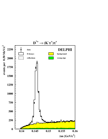
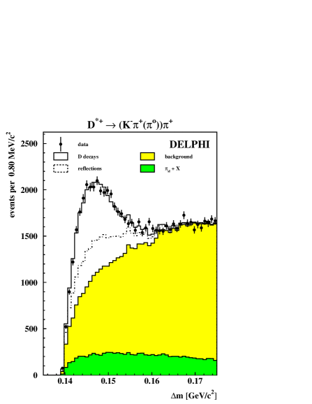
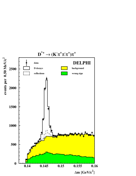
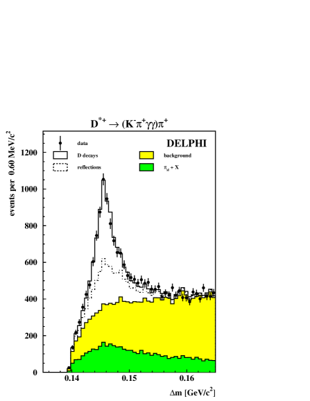
  Figure 1: The mass difference distributions $\Delta$m for the different decay modes. $\Delta$m is defined as the difference between the mass of the $D^{\ast+}$ and the $D^{0}$ candidate. The data are compared to the simulation. Contributions from reflections, partially reconstructed $D^{\ast+}$ decays ($\pi_{sl}+X$) and combinatorial background are also shown. See section 5 for the discussion of these contributions.

  

  

  

  

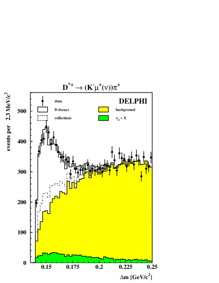
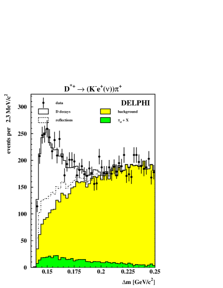
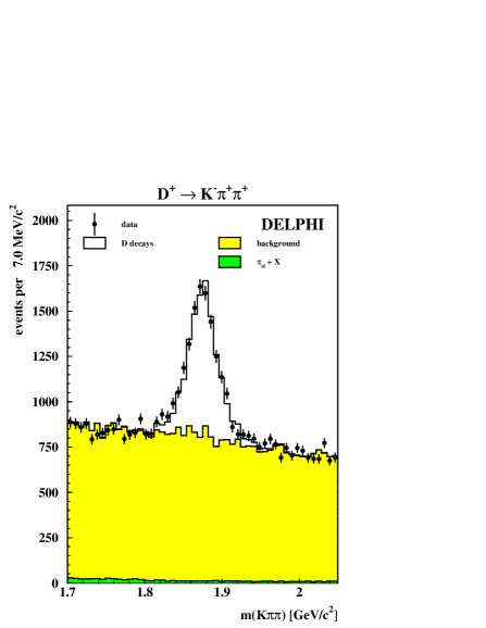
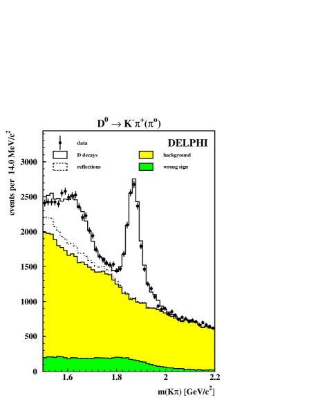
  Figure 2: The mass difference distributions $\Delta$m for the semileptonic decay modes are shown in the two upper plots. $\Delta$m is defined as the difference between the mass of the $D^{\ast+}$ and the $D^{0}$ candidate. The data are compared to the simulation. Contributions from reflections, partially reconstructed $D^{\ast+}$ decays and combinatorial background are also shown. The lower diagrams show the $D^{+}$ and $D^{0}$ mass distributions. For the $D^{0}$ the background distribution for candidates with wrong mass assignments is also shown. In the $D^{0}$ case, the peak in the $K^{-}\pi^{+}$ mass distribution comes from $D^{0}$ decays into $K^{-}\pi^{+}$, and the broad enhancement at lower values is from the $K^{-}\pi^{+}\pi^{0}$ decay.

  

  

  

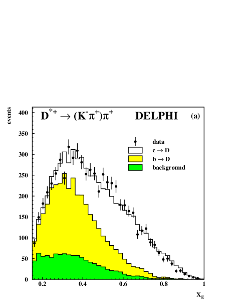
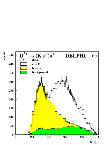
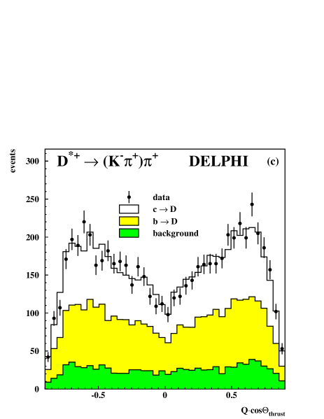
  Figure 3: The $X_{E}$, $tr({\cal P}_{ev})$ and $Q\cdot\cos(\theta_{thrust})$ distribution for the signal region of the $D^{\ast+}\rightarrow(K^{-}\pi^{+})\pi^{+}$ decay mode. The data are compared to the simulation where $D^{\ast+}$ from charm and bottom events and combinatorial background are shown separately. See section 5.1 for the definition of $tr({\cal P}_{ev})$.

  

  

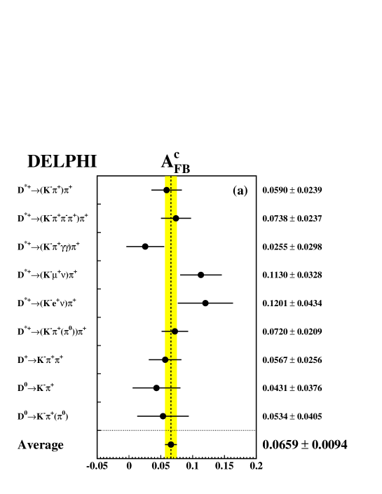
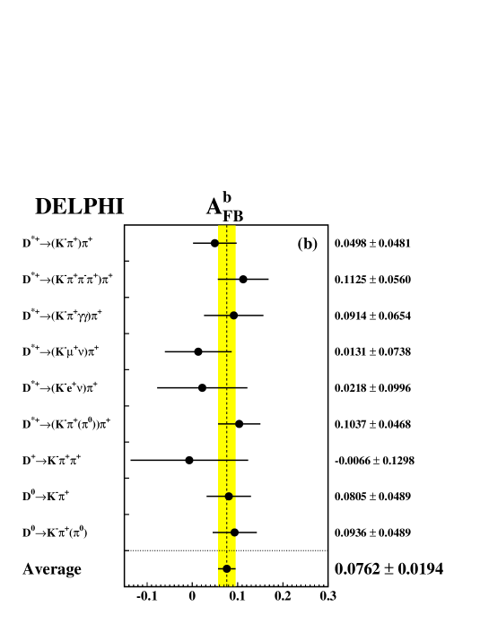
  Figure 4: The results of the two parameter fit of the $c$ and $b$ asymmetry at an average centre–of–mass energy of 91.235 GeV for the different $D$ samples are shown. The grey bands represent the averages over all these measurements. Only statistical errors are shown.

  

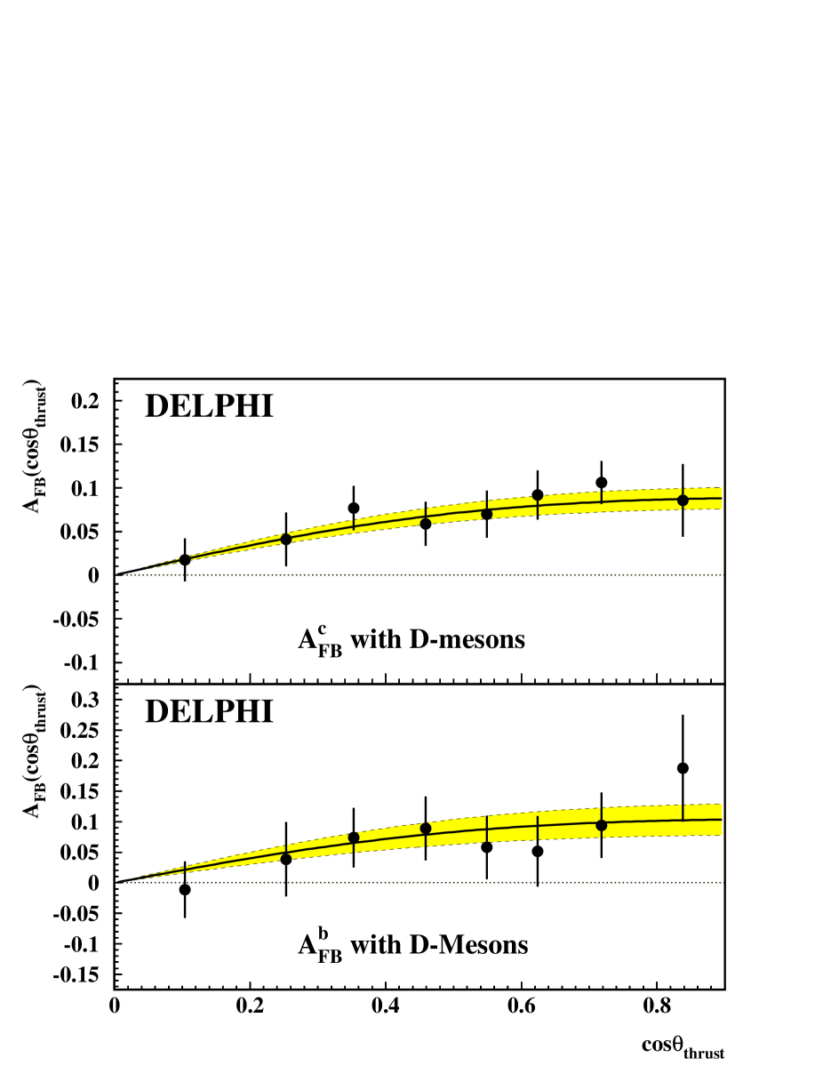
  Figure 5: The $c$ and $b$ forward–backward asymmetries at an average centre–of–mass energy of 91.235 GeV as a function of $\cos\theta_{thrust}$. Only statistical errors are shown. The bands represent the fit results.

  

  

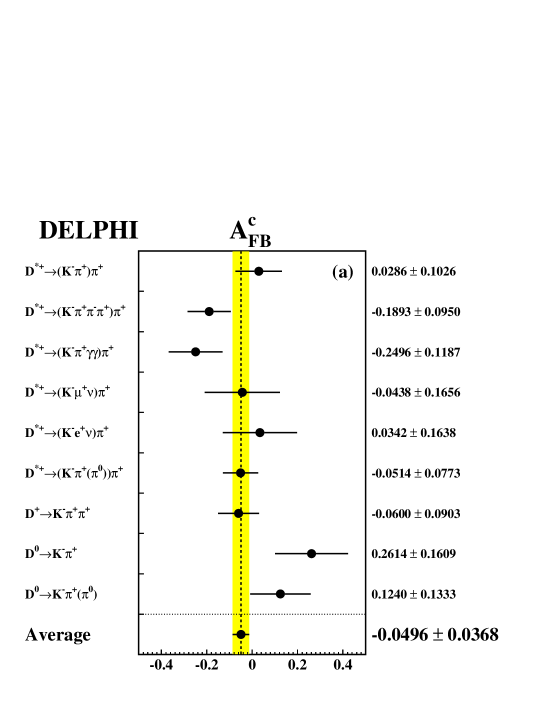
  Figure 6: The results of the two parameter fit of the $c$ and $b$ asymmetry at an average centre–of–mass energy of 89.434 GeV for the different $D$ samples are shown. The grey bands represent the averages over all these measurements. Only statistical errors are shown.

  

  

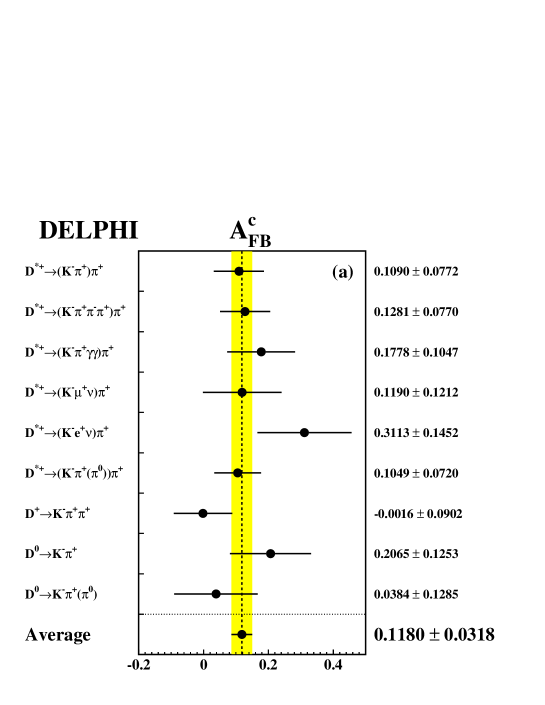
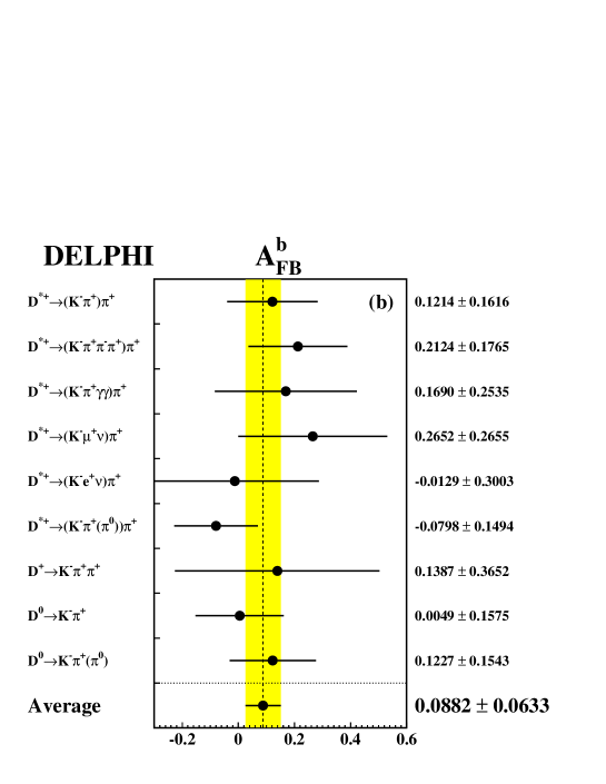
  Figure 7: The results of the two parameter fit of the $c$ and $b$ asymmetry at an average centre–of–mass energy of 92.99 GeV for the different $D$ samples are shown. The grey bands represent the averages over all these measurements. Only statistical errors are shown.

  

  Figure 8: The $c$ and $b$ forward–backward asymmetries for the different average centre–of–mass energies. The SM prediction is also shown (M${}_{Z}=91.187\,{\rm GeV}/c^{2}$, m${}_{top}=175.6\,{\rm GeV}/c^{2}$, m${}_{H}=300\,{\rm GeV}/c^{2}$, $\alpha_{s}({\rm M}_{Z}^{2})=0.120$, $\alpha({\rm M}_{Z}^{2})=1/128.896$).

  Measurement of the forward backward asymmetry
  of $c$ and $b$ quarks at the $Z$ pole
  using reconstructed $D$ mesons