January 1999 IFUP-TH 5/99
hep-lat/9902002

The roughly linear rise of the potential found between adjoint sources in SU($N$) in lattice simulations is expected to saturate into a state of two ‘gluelumps’ due to gluonic screening. We examine this in SU(2) in 2+1 dimensions. Crossover between string-like and broken states is clearly seen by the mixing-matrix technique, using different operators to probe the two states; the breaking behaviour is rather abrupt. Furthermore, we are able to show that both types of operator have a finite overlap with both states; in the case of the Wilson loops the overlap with the broken string is, as predicted, very small.

PACS codes: 11.15.Ha, 12.38.Aw, 12.38.Gc

Keywords: SU(2), lattice, confinement, adjoint representation, mixing, string breaking

1 Introduction

The potential $V(R)$ between sources a distance $R$ apart in SU($N$) gauge theory has been accurately calculated on the lattice for various $N$ and in two and three dimensions and forms a vital ingredient in our understanding of quark confinement. In the case of the potential between fundamental sources, i.e. a quark and an antiquark, one expects the potential to saturate due to pair creation in the vacuum; in the case of sources in the adjoint representation of SU($N$), the potential should also saturate, this time due to screening by gluonic fields. Seeing both these effects is an important step to understanding confinement phenomenology.

However, until recently both have proved elusive. To see any kind of screening of the fundamental potential requires a full QCD simulation with sea quarks, which is still difficult. The best simulations of real-world QCD to date [1] still have fairly heavy quarks and standard potential calculations do not show a clear sign of string breaking.

Two ways have been suggested of improving the situation. Rather than simply asking if the adjoint string breaks, one needs to know: (i) whether states for both broken and unbroken strings exist; (ii) what is the ground state of $V(R)$ as $R$ increases; (iii) what happens if, as we expect, the states cross over. So one should ensure one has a suitable basis of operators for both the broken and unbroken string [2]. Since Wilson loops, the standard probe for the gluonic field, appear to probe the broken string only very poorly, and conversely operators more resembling the broken string are not good probes for the complete one, one can look at mixing between these operators to try and reconstruct the real ground state, using the diagonalisation method originally proposed in ref. [3]. In the case of string breaking, success has been obtained in various models [4, 5], although not yet in full 3+1-dimensional QCD.

Secondly, one can look at Wilson loop operators in a regime where they may be better able to resolve the broken state. By the use of improved actions, enabling the use of coarser lattices, together with a space–time asymmetry, enabling a short time separation for resolving effective masses, Trottier has for the first time found unambiguous evidence of string breaking in full 2+1-dimensional QCD without resorting to mixing matrices [6].

Our intention here is to apply these ideas to the case of the adjoint potential. In this case string breaking was seen using the mixing-matrix approach some time ago in 3+1 dimensions by Michael [7], but a more detailed examination is certainly due. In particular, little evidence was then found for mixing between the broken and unbroken states. In this work we perform simulations in 2+1 dimensions, where the statistics are more in our favour but the physics of confinement appears similar to the 3+1-dimensional case [8]. A study using Wilson loop operators without taking account of mixing found essentially no sign of the broken string [9]. Here we shall use a more complete basis of operators and suggest that when we do this there is little mystery about the breaking of the adjoint string.

In the next section, we describe our method; then we present some initial results on the scaling behaviour of the string tension and of gluelumps to help us choose parameters for the main simulations. The main results are presented in the fourth section; finally we give a brief summary of our conclusions.

2 Method

We consider standard SU(2) lattice gauge theory, but in addition to the Wilson action we have also used the asymmetric improved action [10]:

$$S\equiv\beta\xi\big{(}\frac{5}{3u_{s}^{4}}W_{\mathrm{sp}}+\frac{4}{3\xi^{2}u_{s}^{2}u_{t}^{2}}W_{\mathrm{tp}}-\frac{1}{12u_{s}^{6}}W_{\mathrm{sr}}-\frac{1}{12\xi^{2}u_{s}^{4}u_{t}^{2}}W_{\mathrm{str}}\big{)}.$$ (1)

$W$ are various forms of Wilson loop, $W_{c}=1/2\operatorname{Tr}U_{c}$ where $U_{c}$ is the product of link matrices corresponding to the loop shape $c$. The shapes are, respectively, spatial plaquettes (all links in one of the two space directions), temporal plaquettes (one pair of links in the time direction), spatial rectangles, and short temporal rectangles where the single lattice spacing link is always in the time direction. $\xi$ is the anisotropy, i.e. the ratio of lattice spacings $a_{t}/a_{s}$, and $u_{s}$ and $u_{t}$ are factors inserted for a mean field improvement; as justified below, we have in fact set both of these to unity in our main simulations. As usual, $\beta$ is the inverse coupling $4/g^{2}$. This action has errors of $\mathcal{O}(a_{t}^{2})$, which are small because they are suppressed by a factor $\xi^{4}$. The tree level action $u_{s}=u_{t}=1$ has errors $\mathcal{O}(a_{s}^{2}g^{2})$; the mean field improvement is designed to reduce as much as possible terms of the form $\mathcal{O}(a_{s}^{2}g^{n})$. The standard Wilson action is recovered by taking just the first two terms in the parentheses with coefficient $\beta$. From now on, we take $a\equiv a_{s}$ as the basic lattice spacing.

A simpler form of improvement is to take the temporal part to have the same coefficients as the spatial part, i.e. $5/3$ for all plaquettes and $1/12$ for all rectangles, as done in ref. [6]. We shall refer to this as ST-improvement (for both space and time) to distinguish it from the S-improvement of eqn. (1). The latter has the advantage that only single links occur in the time direction, which keeps the transfer matrix simple. The effects of the higher modes in the ST-form are most apparent when looking at the overlaps of loop operators with physical states, as the coefficients are no longer positive definite. In this work the overlaps are particularly important, so all our improved results use the S-type.

Updating of the lattice was done by a Kennedy–Pendleton heatbath [11] with (after equilibration) four sweeps of exact over-relaxation between each heatbath sweep.

Figure 1: The operators used for probing (a) a magnetic and (b) an electric gluelump. In each case, the fields start and finish at the same site and all the squares are open plaquettes.

To look at both broken and unbroken strings, we use different sets of operators. All quantities in the following discussion are in lattice units. For our broken string operators, the method follows that originally described in full in 3+1 dimensions in ref. [12] and used in early work on the adjoint sector [13]. As briefly mentioned above, the broken adjoint string is expected to resemble a pair of gluelumps, each of which is a localised static gluonic field surrounded by dynamical gluons. This is because of the static spatial part of the Wilson loop; in the real world, no such source exists and the pure glue states are glueballs, i.e. states with an indeterminate number of purely dynamical gluons. However, gluelumps, when they can form, are considerably lighter. In two spatial dimensions, there are two types of gluelump with distinct quantum numbers, ‘magnetic’ and ‘electric’, whose masses were calculated in ref. [9] by essentially the method we are adopting. Suitable operators can be made from combinations $G_{i}$ ($i$ standing for magnetic or electric) of ‘open’ plaquettes (i.e. the SU(2) matrix corresponding to the complete path before the trace is taken) as shown in fig. 1. We could in principle use larger Wilson loops than plaquettes, but results are entirely satisfactory when combining the use of plaquette operators with the fuzzing prescription described later.

The operators $G_{i}$ are traceless, as the individual parts have $C=-1$ and the trace of an SU(2) matrix is real so has only $C=+1$. Thus before we can measure anything we need to combine the two parts in a gauge-invariant way using temporal links. Finally, we need a trace in the adjoint representation. More formally, the complete operator $\mathcal{G}$ [12] consists of

$$\mathcal{G}_{i}(T)=\operatorname{Tr}(G_{i}(0)\sigma^{a})A^{ab}(U(0,T))\operatorname{Tr}(G_{i}^{\dagger}(T)\sigma^{b}),$$ (2)

where $U(0,T)$ is the product of links between $G_{i}(t=0)$ and $G_{i}(t=T)$; $t$ and $T$ will be taken in lattice units, i.e. they count temporal lattice spacings. For the adjoint projection $U$ is combined in the form,

$$A^{ab}(U)=\frac{1}{2}\operatorname{Tr}(\sigma^{a}U\sigma^{b}U^{\dagger}).$$ (3)

Here, the $\sigma^{a}$ are the Pauli matrices, $a=1\dots 3$, and the standard identity

$$\sigma_{ij}^{a}\sigma_{kl}^{b}=2(\delta_{il}\delta_{jk}-\frac{1}{2}\delta_{ij}\delta_{kl})$$ (4)

means that $\mathcal{G}$ has the simple form

$$\mathcal{G}_{i}(T)=2\operatorname{Tr}(G_{i}(0)U(0,T)G_{i}^{\dagger}(T)U^{\dagger}(0,T)),$$ (5)

since as already indicated the traces of the $G_{i}$ vanish. This ‘dumbbell’ operator, corresponding to creation of a gluelump and its annihilation after time $T$, allows us to measure the gluelump mass in the usual way. The broken string state is modelled by two of these $\mathcal{G}_{i}$ separated by some distance $R$; for large enough $R$ in the confined phase this will overlap predominantly onto a state of twice the mass of the individual gluelump. We shall refer to it in what follows as the ‘two-dumbbell operator’, to distinguish from the physical state of two gluelumps that we expect it to resemble at least for large $R$. We shall also use the shorthand ‘two magnetic dumbbells’ which is to be interpreted as two such operators, each with the quantum numbers of a magnetic gluelump.

The operator for the adjoint potential from Wilson loops $W_{\mathrm{adj}}(R,T)$ corresponding to the unbroken string distance $R$ apart propagating for time $T$ comes simply from calculating the loop in the usual way then taking the adjoint trace,

$$\operatorname{Tr}_{\mathrm{adj}}U_{c} \equiv\frac{1}{3}(4\operatorname{Tr}_{\mathrm{fund}}^{2}U_{c}-1),$$ (6)

$$\operatorname{Tr}_{\mathrm{fund}}U_{c} \equiv\frac{1}{2}\operatorname{Tr}U_{c},$$ (7)

where $U_{c}$ is the matrix product of the links corresponding to the closed path $c$. It is thus simple to keep the fundamental potential for comparison.

Finally, to calculate mixing between the states we follow exactly the method of ref. [4], but replacing the scalar meson operators with the operators $G_{i}$ and the fundamental with adjoint fields. Then we need operators corresponding to an unbroken string developing into a two-gluelump state or vice versa. These can be seen in the off-diagonal parts of the matrix in fig. 2. They are identical to the operators $G_{i}$, except with a different shape to the links, so we again use eqn. (5) with $U(0,T)$ replaced by the appropriate ‘U’-shaped product of links, and with the $G_{i}$ spatially instead of temporally separated.

All our gluonic operators for measurement use the now standard iterative ‘fuzzing’ prescription [14], in which a spatial link is replaced recursively by a sum of the original link and the four three-link spatial staples around it, preserving the lattice symmetry. Our conventions for the constants are, in condensed form,

$$U^{(n_{f}+1)}(x,\mu)=P\{c_{f}U^{(n_{f})}(x,\mu)+\sum_{\nu\neq\mu}\mathrm{staples}^{(n_{f})}(x,\mu,\pm\nu)\}$$ (8)

where $P$ represents a projection back to SU(2) for numerical convenience, the staples are the four matrices representing the possible three-link paths from position $x$ to $x+\hat{\mu}$ going first in either the $+\nu$ or $-\nu$ direction, and $U^{(n_{f})}(x,\mu)$ is a link matrix after $n_{f}$ iterations of fuzzing, where the original links are those for $n_{f}=0$. The choice of the coefficient of the original link $c_{f}$ and the number of iterations need to be tuned to maximise the overlap to physical states. In addition to improving the overlap, this also provides us with different trial operators for the mixing matrix.

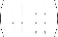
Figure 2: Schematic depiction of the states in the mixing matrix $M(R,T)$; each filled circle represents one of the operators of fig. 1, and all links are taken in the adjoint representation. In each state shown $R$ is horizontal and $T$ vertical.

The resulting mixing matrix $M(R,T)$ is shown schematically in fig. 2; different fuzzing levels are also included for each type of operator. The off-diagonal terms in the full matrix consist in taking the appropriate product of links or pair of local operators at $t=0$ and at $t=T$: for example, the pure Wilson loop part of the matrix includes an unfuzzed product of links at $t=0$ together with a fuzzed product at $t=T$, and so on. Note that we always use a given fuzzing level for a given timeslice, so that both gluelumps in the off-diagonal operators of fig. 2 always have the same fuzzing.

We then need to diagonalise the corresponding transfer matrix [3]. Ideally, we wish to have

$$M^{\prime}(R,T+1)\lvert\psi(R)\rangle=\operatorname{diag}(C_{0}(R)\exp(-m_{0}(R)a_{t}),\quad C_{1}(R)\exp(-m_{1}(R)a_{t}),\quad\dots)\\ M^{\prime}(R,T)\lvert\psi(R)\rangle$$ (9)

for the spectrum of states $\psi_{i}(R)$ with masses $m_{i}(R)$ and some coefficient $C_{i}(R)$. Actually, we have only a truncated basis and finite statistics and can only hope for an approximation to this, which we arrange by solving the corresponding eigenvalue problem for the original $M(R,T)$ and $M(R,T+1)$ for each $R$ separately. Thus we need to pick a basis $(T_{D},T_{D}+1)$ for the process. Various factors come into this: first, operators have smaller relative errors at lower $T_{D}$; second, the contaminating effect of higher states which cannot fit into our finite basis is less at larger $T_{D}$; finally there may be low-lying states with small coefficients $C_{i}(R)$ which are swamped at small $T_{D}$, but which are clearer when we go to larger $T_{D}$.

We use the notation $C(R,t)$ to indicate the set of diagonalised correlation functions,

$$C_{i}(R,t)=C_{i,0}(R)\exp(m_{0}(R,t))+C_{i,1}(R)\exp(m_{1}(R,t))+\dots$$ (10)

where the subscript $i$ is an index for the eigenvalue taken in the diagonalisation. After the diagonalisation, only one $C_{i,j}(R)$ should dominate for each, at least for the lowest states, and we order the eigenvalues so that this is $C_{i,i}(R)$. We consider the first two eigenmodes in each case, which (barring problems in the numerical procedure) give the lowest two masses $m_{0}(R)$ and $m_{1}(R)$. We then fit a single exponential to $C_{i}(R,t)$ starting from some $t$ to be decided later: all our fits use a correlated $\chi^{2}$, where errors are determined by the bootstrap method. If the fit is acceptable, then the calculated coefficient $C_{i,i}(R)/C_{i}(R,0)$ gives an estimate of the overlap of the operator basis with the physical state, something of particular interest in the present case; this is the quantity meant when we talk of overlaps in what follows. From basic quantum mechanics the overlaps onto the basis of states are positive and sum to one (again, barring numerical problems) for both our actions. We also define the effective mass for a given $R$ in the usual way,

$$m_{\mathrm{eff}}(t)=-\log(C(t)/C(t+1)),$$ (11)

a useful indication of whether a single exponential term dominates. However, it should be noted that the masses quoted are from the fit to the exponential, not effective masses, to allow us a reasonable estimate of the overlap.

For the temporal links in the Wilson (but not the improved) case we have used the so-called ‘multihit’ technique [15] to improve statistics, though in the case of SU(2), where the improved link can be calculated exactly, the name ‘single bullseye’ would be more appropriate. In this method we can perform an analytic integration on half of the temporal links (all those which have no plaquette in common), replacing them by

$$U_{l}\longrightarrow U_{l}^{\prime}=\frac{I_{2}(\beta k_{l})}{I_{1}(\beta k_{l})}V_{l},$$ (12)

where $I_{n}(x)$ is a modified Bessel function, $k_{l}V_{l}$ is the sum of the four three-link ‘staples’ surrounding the original link $U_{l}$ with the same start and end point such that $k_{l}$ is a positive real number and $V_{l}$ is a (uniquely determined) SU(2) matrix. Expressions involving the right hand side of eqn. (12) have the same expectation value but with less noise. Note that this expression is for the fundamental representation; for the adjoint case one can use the same improved matrices but when taking an adjoint trace as in eqn. (7) instead of subtracting $1/3$ from $4\operatorname{Tr}_{\mathrm{fund}}^{2}(U_{c})/3$, one must subtract $\operatorname{Tr}({U_{c}^{\prime}}^{\dagger}U_{c}^{\prime})/6$; this is easily implemented. There is also a particularly simple method for calculating the $I_{n}(x)$ required, namely via the recurrence relation

$$I_{n-1}(x)=I_{n+1}(x)+\frac{2n}{x}I_{n}(x),$$ (13)

using the fact that the $I_{n}(x)$ decrease with increasing $n$. Starting from some high $n$ (we have found $n=17$ sufficient for 32-bit precision), we take $I_{n+2}(x)=0$ and $I_{n+1}=\epsilon$ for some arbitrary but small $\epsilon$, and work backwards. This gives $I_{2}(x)$ and finally $I_{1}(x)$ up the same overall constant factor, so we simply divide the results obtained for the two to obtain $I_{2}(x)/I_{1}(x)$. In the S-improved case, where the action is more complicated and more links are involved, we have not attempted to modify the multihit algorithm appropriately and so have not used it.

3 Choice of actions and lattices

We wish to see if coarse lattices are as useful as they are in the case of breaking of the fundamental string [6]. For this we would first like some idea of the behaviour of the S-improved actions in this region. It is customary to use the fundamental string tension $K$ for setting the scale, which has a proper continuum limit. In the Wilson case there is already ample data for this [8]. We also calculate the masses of the two lowest-lying gluelumps with both magnetic and electric quantum numbers for comparison. As a static source, these have logarithmic divergences [16], so that there is no continuum limit for the bare gluelump masses, nor is there a simple scaling behaviour. However, the adjoint potential in which we are interested consists of two such static sources and hence twice the gluelump mass is an aid to matching the potential at different $\beta$.

In 2+1 dimensions, the fundamental potential has a long range Coulombic part which is logarithmic, making it difficult to separate out the linear effect of the string tension. We have followed ref. [8] and determined $K$ from correlations of the Polyakov loop $\operatorname{Tr}U_{P}(t)$, which wraps around the spatial boundary at some $t$ and hence has length $N_{s}$ units on an $N_{s}^{2}N_{t}$ lattice. Including the appropriate form of the universal string correction [17, 18], the asymptotic form is

$$\langle\operatorname{Tr}U_{P}(0)\operatorname{Tr}U_{P}(T)\rangle@>t\to\infty>>\exp-\left(Ka-\frac{\pi}{6aL}\right)\xi at,$$ (14)

where $K$ is the string tension and the lattice spacing $a$ and anisotropy $\xi$ have been shown explicitly.

For the improved action we have concentrated on small $\beta$, and for the Wilson action on larger $\beta$, reflecting the regions where we expect to use each action. The effect of $u_{t}$ is expected to be slight and we have set it everywhere to unity. In choosing lattice sizes, we have had an eye to the results of ref. [8], and in particular fig. 9 which appears to indicate that a lattice dimension of $24$ at $\beta=9$ is sufficient to eliminate finite size effects in the low-lying glueball spectrum. We have assumed approximate asymptotic scaling of the string tension, which is obeyed closely enough for this purpose, to adjust lattice sizes to have roughly this physical volume as a minimum.

$\beta$	$\xi$	Size	$u_{s}^{4}$	$Ka^{2}$	$\beta\sqrt{\!K}$
2.0	0.25	$6^{2}\times 32$		0.52(2)	1.44(3)
2.0	0.25	$8^{2}\times 32$		0.48(4)	1.38(5)
2.0	0.25	$12^{2}\times 32$		0.50(13)	1.4(2)
2.5	0.25	$8^{2}\times 32$		0.303(1)	1.38(2)
2.5	0.25	$10^{2}\times 32$		0.321(16)	1.42(4)
2.5	0.25	$12^{2}\times 32$		0.33(2)	1.44(5)
3.0	0.25	$8^{2}\times 32$		0.226(8)	1.43(3)
3.0	0.25	$12^{2}\times 32$		0.23(1)	1.43(3)
3.0	0.25	$16^{2}\times 32$		0.217(15)	1.40(4)
3.0	0.333	$8^{2}\times 32$		0.214(11)	1.39(4)
3.0	0.333	$12^{2}\times 32$		0.236(13)	1.46(4)
3.0	0.333	$16^{2}\times 32$		0.23(2)	1.43(8)
2.0	0.25	$6^{2}\times 32$	0.605	0.304(7)	1.103(13)
2.0	0.25	$8^{2}\times 32$	0.605	0.273(9)	1.044(16)
2.0	0.25	$12^{2}\times 32$	0.605	0.37(17)	1.2(3)
3.0	0.25	$8^{2}\times 32$	0.767	0.160(5)	1.20(2)
3.0	0.25	$12^{2}\times 32$	0.767	0.167(5)	1.23(2)
3.0	0.25	$16^{2}\times 32$	0.767	0.170(8)	1.24(3)

Table 1: String tensions in lattice and asymptotic units extracted using eqn. (14) on various lattices with the S-improved action of eqn. (1).

$\beta$	Action	$\xi$	Size	$u_{s}^{4}$	$M_{\mathrm{gm}}^{(0)}$	$M_{\mathrm{gm}}^{(1)}$	$M_{\mathrm{ge}}^{(0)}$	$M_{\mathrm{ge}}^{(1)}$
3.0	W	0.5	$16^{2}\times 32$		1.95(2)	2.91(3)	2.26(3)	3.14(14)
5.0	W		$16^{3}$		1.192(6)	1.71(3)	1.466(13)	1.81(4)
6.0	W		$32^{3}$		0.996(3)	1.422(6)	1.235(3)	1.55(3)
7.0	W		$24^{2}\times 32$		0.851(4)	1.21(3)	1.09(3)	1.40(4)
8.0	W		$24^{2}\times 32$		0.747(5)	1.072(16)	0.95(2)	1.16(6)
9.0	W		$24^{2}\times 32$		0.670(3)	0.96(3)	0.81(2)	1.21(15)
2.0	SI	0.25	$6^{2}\times 32$		2.508(16)	3.96(6)	2.82(2)	3.97(6)
2.0	SI	0.25	$8^{2}\times 32$		2.504(8)	3.90(3)	2.82(3)	4.06(3)
2.0	SI	0.25	$10^{2}\times 32$		2.508(12)	3.96(3)	2.828(2)	4.00(4)
2.0	SI	0.25	mean		2.504(8)	3.93(2)	2.824(8)	4.02(2)
2.5	SI	0.25	$8^{2}\times 32$		1.976(8)	3.02(2)	2.364(8)	2.97(8)
2.5	SI	0.25	$10^{2}\times 32$		1.972(8)	3.00(2)	2.364(8)	3.13(2)
2.5	SI	0.25	$12^{2}\times 32$		1.982(5)	2.90(5)	2.372(8)	3.124(12)
2.5	SI	0.25	mean		1.978(4)	3.004(12)	2.368(4)	3.124(8)
3.0	SI	0.25	$8^{2}\times 32$		1.660(8)	2.48(2)	2.04(2)	2.65(2)
3.0	SI	0.25	$12^{2}\times 32$		1.664(8)	2.516(8)	2.051(6)	2.664(8)
3.0	SI	0.25	$12^{2}\times 36$		1.656(3)	2.476(8)	2.041(6)	2.664(8)
3.0	SI	0.25	$16^{2}\times 32$		1.648(4)	2.472(8)	2.052(4)	2.640(12)
3.0	SI	0.25	mean		1.653(2)	2.488(4)	2.050(3)	2.652(4)
3.0	SI	0.33333	$8^{2}\times 32$		1.659(9)	2.50(2)	2.046(12)	2.66(2)
3.0	SI	0.33333	$12^{2}\times 32$		1.656(6)	2.490(12)	2.046(6)	2.66(2)
3.0	SI	0.33333	$16^{2}\times 32$		1.660(4)	2.499(9)	2.08(2)	2.77(5)
3.0	SI	0.33333	mean		1.659(3)	2.496(6)	2.049(6)	0.888(4)
4.0	SI	0.33333	$16^{2}\times 36$		1.278(6)	1.926(12)	1.64(2)	0.734(9)
5.0	SI	0.5	$16^{2}\times 32$		1.046(4)	1.58(2)	1.328(6)	1.84(2)
2.0	SI	0.25	$6^{2}\times 32$	0.605	2.028(12)	3.28(12)	2.47(3)	3.1(2)
2.0	SI	0.25	$8^{2}\times 32$	0.605	2.004(12)	3.22(2)	2.47(2)	3.28(6)
2.0	SI	0.25	$12^{2}\times 32$	0.605	2.032(12)	3.16(2)	2.49(2)	3.36(4)
2.0	SI	0.25	mean	0.605	2.020(8)	3.21(2)	2.480(12)	3.316(12)
3.0	SI	0.25	$8^{2}\times 32$	0.767	1.528(12)	2.48(4)	1.93(2)	2.76(3)
3.0	SI	0.25	$12^{2}\times 32$	0.767	1.508(8)	2.50(2)	1.972(8)	2.68(4)
3.0	SI	0.25	$16^{2}\times 32$	0.767	1.528(8)	2.46(2)	1.964(12)	2.72(3)
3.0	SI	0.25	mean	0.767	1.520(4)	2.48(2)	1.968(8)	2.72(2)
4.0	SI	0.33333	$16^{2}\times 32$	0.7735	1.176(6)	1.79(2)	1.497(12)	2.03(4)
5.0	SI	0.5	$16^{2}\times 32$	0.824	0.986(2)	1.44(2)	1.256(6)	1.68(4)

Table 2: Gluelump masses for Wilson action (W) and for the S-improvement of eqn. (1) (SI) with and without mean field improvement ($u_{s}$). The two lowest-lying magnetic and the two lowest-lying electric gluelumps are shown.

Results for the string tension are shown in table 1. In most cases they are for about 1000 configurations, though more were available from the runs to be described in the main section on adjoint string breaking. Where $u_{s}\neq 1$, we adjusted it in a self-consistent fashion until the spatial plaquette was $u_{s}^{4}$ to the accuracy shown; if it is not shown, $u_{s}=1$.

All mass values are given in spatial units; to convert from the temporal units in the correlator we have simply divided by the tree-level asymmetry $\xi$ given in the second column. This is not necessarily correct, as there could be renormalisations to $\xi$. However, in our later calculations we will only require masses consistent on a given set of lattices, and the factor $\xi$ appears consistenly in front of all masses in exponentials of the form $\exp(-ma\xi t)$, so this is not a major concern for us.

If asymptotic scaling holds, then $\beta$, which in 2+1 dimensions has the dimensions of length, also scales; we test this in the final column of the results by constructing the dimensionless quantity $\beta\sqrt{\!K}$. It was found for the Wilson case with $\beta$ down to around 6 that the results fit a single linear violation of asymptotic scaling [8], with an intercept at $1/\beta=0$ of $1.341(7)$, while the ST-improvement of ref. [6] shows virtually no sign of any violation of asymptotic scaling even without mean-field improvement down to $\beta=2$; this effect, much more striking than in 3+1 dimensions, may be related to the fact that the theory in our case is superrenormalisable.

Figure 3: The string tension $K$ for various actions, shown in units $\beta\sqrt{K}$ against $1/\beta$. The Wilson results are from ref. [8]. Note that the tree-level asymmetry $\xi$ has been used to calculate the improved masses; this may undergo renormalization.

These results are plotted against $1/\beta$ in fig. 3. Where the results are consistent, only a weighted mean of results from different lattice volumes is shown. Those without the mean-field improvement, i.e. $u_{s}=1$, show no clear trend in either volume or $\beta$ and cluster around $\beta\sqrt{\!K}=1.40$ to $1.43$. This suggests a roughly universal behaviour, which, however, is slightly above the value $1.341(7)$ quoted above. This may be due to the renormalization in $\xi$ mentioned above, which is found [19] to be large in the case without mean-field improvement, so that the real values would be shifted downwards towards the weak coupling limit. However, the presence of approximate scaling apart from this shift is pleasing.

With mean-field improvement, the values are lower, and might already be nearer the weak coupling limit. At $\beta=2.0$ the values for the two smaller volumes are not entirely consistent (the largest volume is not plotted), although this could still be a statistical fluctuation.

Figure 4: The ground-state mass of the magnetic gluelump for various actions, shown in units $\beta M$ against $1/\beta$. Note this is divergent, so one cannot trivially take a continuum limit.

Figure 5: As 4, but for the ground-state mass of the electric gluelump.

For the gluelump masses, the results are shown in table 2, and the product of the masses of the lowest-lying magnetic and electric gluelumps with $\beta$ are plotted in figures 4 and 5 respectively; the comment about $\xi$ above still applies. As already noted, these are divergent and one cannot take a simple continuum limit. Given this, the fact that the graph for the Wilson action is extremely flat — even in comparison with the string tension — is the more surprising, since it is highly unlikely this comes from a coincidental cancellation between lattice artifacts and the divergent contribution. So it would seem both effects are in this region benign.

However, we are not in a position to say the same thing about the improved results, which are considerably shifted from the Wilson values, and, though they show a rough plateau at small $\beta$, drift upwards for large $\beta$, more noticeably in the case of the electric gluelump. The latter is also less well measured, due partly to the higher mass, but also possibly to the operators being better optimised for the magnetic gluelump. The cause of the drift is hard to determine, given all the possible effects.

Furthermore, taken together the plots also indicate the ratio between the magnetic and electric gluelumps at a given $\beta$ is not maintained by the S-improved action for $\beta\lesssim 3.0$, with or without mean-field improvement. All the graphs cast doubt on the benefits of mean-field improvement at the lowest $\beta$, where the results do not fit any obvious trend.

This complicates the choice of action, but in the absence of any better suggestion we shall retain the S-improved action for results at small $\beta$.

4 Adjoint strings: mixing and breaking

Given the results of the previous section, we decided to concentrate on just one coupling in the Wilson case at $\beta=6.0$ and two with the S-improved action, $\beta=3.0$, where scaling in the gluelump sector appears to be just breaking down, and $\beta=2.0$, where we certainly cannot trust scaling. Furthermore, $\beta=2.0$ seemed too small to provide additional mean-field improvement, at least in the way implemented here, and we have kept $u_{s}=1$ for both couplings.

The runs are shown in table 3. We have used three sets of operators: Wilson loops ($\mathcal{W}$), magnetic dumbbells ($\mathcal{M}$), and electric dumbbells ($\mathcal{E}$), with the corresponding combinations for the off-diagonal elements of the mixing matrix. For each operator we used three levels of fuzzing: one was always the raw (unfuzzed) operator (denoted by adding 0 to the operator formed out of the unfuzzed links), one had a small amount of fuzzing (denoted 1), and the third consisted of the optimal amount of fuzzing (denoted 2). The two sets of fuzzing parameters we have used in each case are shown in the table; it should be noted that overlaps with the gluelump states and with the unbroken string are not necessarily optimised by the same set of fuzzing parameters, and our choice was to concentrate on the unbroken string. Hence the full matrix is $9\times 9$, which we abbreviate by indicating the operators and fuzzing levels included as $\mathcal{W}$$\mathcal{M}$$\mathcal{E}$012; we shall use this as a shorthand when indicating the basis. Likewise, $\mathcal{W}$012 indicates a basis of the three levels of fuzzing but from Wilson loops alone; $\mathcal{W}$2 indicates the single most highly fuzzed Wilson loop operator, and so on.

In two cases, once mixing had been clearly seen with the full matrix, we performed further runs with only the Wilson loop operators to try to see if these had some finite overlap with the broken string, which is why we give two sets of configuration numbers.

For the $\beta=6$ run we simply used all the spatial separations along the axis from $R=1$ to 16. We used preliminary results from this to concentrate points in the expected string-breaking region for the two coarser lattices, where we have also used both on- and off-axis points for the spatial separation $R$ in both the Wilson loop and two-dumbbell operators.

				Fuzzing $(n_{f},c_{f})$
$\beta$	Action	$\xi$	Size	Level 1	Level 2	Full configs.	Loop configs.
2.0	S	0.25	$8^{2}\times 32$	$(1,10.0)$	$(4,10.0)$	4500	8500
3.0	S	0.25	$12^{2}\times 36$	$(2,5.0)$	$(6,5.0)$	2000	2000
6.0	W	1	$32^{3}$	$(5,2.3)$	$(30,2.3)$	2200	5900

Operators	Notation
Wilson loop	$\mathcal{W}$
‘Dumbbell’ with magnetic quantum numbers	$\mathcal{M}$
‘Dumbbell’ with electric quantum numbers	$\mathcal{E}$

Table 3: Runs performed in the search for adjoint string breaking. We denote the three types of operator included by the symbols shown, and indicate the fuzzing level by adding $0$ (no fuzzing), $1$ (the first set of parameters given above) or $2$ (the second set). Hence our full set of operators for each run is denoted $\mathcal{W}$$\mathcal{M}$$\mathcal{E}$012, which implies we have used a $9\times 9$ mixing matrix of the form shown schematically in fig. 2.

First we need to choose a diagonalisation basis $(T_{D},T_{D}+1)$ as described above. $T_{D}=0$ is not a useful choice, as the Wilson loops all have area zero and hence the matrix $M(R,0)$ consists of many degenerate elements equal to unity, so we have tried $T_{D}=1$ and larger. In principle we could pick $T_{D}$ separately for each diagonalisation. In practice we have found no case where $T_{D}>1$ improves the result of the calculation, and many are made unstable by this choice — particularly those where the errors on $C(R,T_{D})$ are significant, which are just those cases we are most interested in seeking an improvement. Hence all our results use $T_{D}=1$.

Our effective mass plateaus thus obtained are in most cases very good, with $m_{\mathrm{eff}}(t=2)$ already close to the plateau value for the Wilson data, and we are clearly able to calculate the two lowest masses in the majority of cases. In the results shown, we have decided point by point at what time value the fit to the exponential should start by considering both the $\chi^{2}$ per degree of freedom and the flatness of the plateau, to try to be reasonably but not excessively conservative. All use either $t=2$, 3 or 4.

Results from full mixing matrix

Figure 6: The results for the adjoint potential including all operators ($\mathcal{W}$$\mathcal{M}$$\mathcal{E}$012) at $\beta=6.0$, Wilson action, showing the first two states, as well as the twice the masses of the two lowest gluelumps. Diagonalisation has failed for the excited state at small distances.

Figure 7: The results for the adjoint potential including all operators ($\mathcal{W}$$\mathcal{M}$$\mathcal{E}$012) at $\beta=3.0$, improved action showing the first two states, as well as the twice the mass of the lowest magnetic gluelump. Note the narrower range of distances in comparison with fig. 6.

Figure 8: The lowest state adjoint potential from all operators ($\mathcal{W}$$\mathcal{M}$$\mathcal{E}$012), showing all three sets of data rescaled to $\beta=6$ as described in the text.

The results for the two lowest-lying states of the adjoint potential from the complete basis of 9 operators ($\mathcal{W}$$\mathcal{M}$$\mathcal{E}$012) are shown in fig. 6 (Wilson at $\beta=6.0$) and fig. 7 (S-improved at $\beta=3.0$); in each case, twice the mass of the lowest-lying gluelump or gluelumps is shown as a straight line.

The complexities of scaling referred to above make it hard to overlay these graphs. First we rescale all points according to the string tension; this leaves the matter of the divergence of the two static sources, corresponding to a vertical shift of the potentials at different $\beta$. As the plateau can be clearly seen to correspond to the mass of two magnetic gluelumps, we have then shifted the vertical axis by eye until the plateaus roughly correspond (we do not here need the extra accuracy a full fit would give). With good scaling behaviour, this procedure should be qualitatively correct. This is attempted in fig. 8; the labels of the axes show the values for the $\beta=6$ run. The point at which the string breaks seems to be roughly universal, although the rising parts of the potential do not agree very well.

At $\beta=6.0$ the diagonalisation has failed for $R\lesssim 5$, where it was not able to separate the first excited state from the ground state; a similar tail appears in the $\beta=3.0$ data, which again probably represents failure of the procedure rather than anything physical (note fig. 7 does not go to such short distances as fig. 6). A possible clue as to why this should happen is that the ‘U’-shaped operators forming the off-diagonals in fig. 2 have themselves a strong overlap with the unbroken string at short distances, approaching unity as $R\to 0$, hence it may become more difficult to resolve the excited two-gluelump state from the full set of operators; however, even the two-dumbbell operators alone have difficulties in this region, as described below.

Notwithstanding the problems, the overall effect is clear; one sees not one but two string breakings, as the first excited potential itself flattens off at the value of twice the mass of the lowest-lying electric gluelump. The effect is very stark; there seems to be very little sign of ‘repulsion’ between the two curves at the crossover point, as is commonly associated with such phenomena, a point already noted in ref. [7], although the picture is qualitatively similar to that seen in breaking of a fundamental string to two scalar mesons [4, 5]. It is clear here, as there, that the mass of the particle in the broken state is the major factor determining the breaking scale, which can be read of in lattice units from the horizontal axis.

We performed initial fits during the diagonalisation; these give us a way of estimating the overlap of the original operators with both of the first two states. Since two-exponential fits are notoriously difficult, we first fit a single exponential to each of the lowest two eigenmodes; these are essentially the same fits as those used to extract the potential itself. We then make a two-exponential fit to the original data sets for the individual operators, but with the masses fixed to the values obtained from the first fit so that only the two coefficients are free. This will not work if one has reason to think the data in question have a significant overlap with a third exponential; we have not actually identified any third state to see if this is the case. Of course, the whole diagonalisation procedure is anyway at the mercy of effects from badly resolved states.

Figure 9: Overlap of the most highly fuzzed Wilson-loop operator ($\mathcal{W}$2) with the ground state (circles) and first excited state (squares) of the adjoint potential for $\beta=3.0$.

Figure 10: As fig. 9, but showing the overlaps of the most highly fuzzed two-magnetic-dumbbell operator ($\mathcal{M}$2).

This has worked most successfully for the $\beta=3.0$ data, possibly because the combination of coupling and asymmetry give it the longest plateaus. In fig. 9 we show the overlap of the most highly fuzzed loop operator ($\mathcal{W}$2) with the ground state and the first excited state of the potential, and in fig. 10 we show the corresponding graph for the operator consisting of two magnetic dumbbells, again with the highest fuzzing ($\mathcal{M}$2). As one would expect, these complement one another nicely, with a clear crossover around $R=5.2a$. The crossover of the overlaps appears less abrupt than that in the states themselves, again in accordance with the results of ref. [4]. In the region where the states have similar masses, it may be difficult for the diagonalisation to separate the first two states; this presumably explains why in fig. 9 immediately after string breaking the overlap for the excited state is too high and that for the ground state too low.

Results from individual types of operator

The problem that started this project was the difficulty (even apparent impossibility) of seeing string breaking in Wilson loop operators alone and figs. 9 and 10 have confirmed our expectations that each operator is linked particularly with either the unbroken or the broken string, but not both. It is therefore interesting to see if one can detect any finite overlap, however small, of the operators with the ‘wrong’ states.

Figure 11: Above, the adjoint potential from diagonalisation of the three operators consisting of two magnetic dumbbells ($\mathcal{M}$012) at $\beta=6$ for the ground state (circles) and first excited state (squares). Below, the overlap with the states resolved.

It turns out that the overlap of the two-dumbbell operator with the unbroken string at small distances is large enough to produce quite reasonable results. The behaviour for the three operators consisting of two magnetic dumbbell at $\beta=6.0$ ($\mathcal{M}$012) is shown in fig. 11; here we have diagonalised just the three relevant data channels in the mixing matrix — note the difference from fig. 10 where we showed the overlap for a single operator of this type. For the lowest state, the change between projecting the unbroken and broken string is very clear, with large errors in the region where it is hard to separate the two states; in particular, the unbroken string is not followed for $R\gtrsim 5a$, as it should intersect the two-gluelump plateau around $R=10a$ (compare fig. 6).

For the overlaps with the state resolved, also shown in fig. 11, this time we have simply used the coefficient of a single exponential fit. At small $R$, where the string-like state is resolved, the overlap starts at around $20\%$ and decreases, then increases suddenly where the broken state dominates. This is, indeed, our most striking evidence that particular operators can have significant overlaps with both the broken and unbroken string. A similar picture appears for the other data sets, but is less striking as the points are concentrated around the region of string breaking.

We have already seen that with the complete basis the procedure does not work well for the excited state at short distances, so it is questionable whether the corresponding part of fig. 11 shows a physical state, rather than merely an artifact of the method: the overlap is much lower than that where the two-gluelump state is well resolved, although higher than with the ground state. The diagonalisation procedure is unable to resolve the two states separately in the crossover region where the string-like and broken states have similar masses. For large $R$, where the operators resolve two broken-string states, the mass of the excited state corresponds to twice the lowest electric gluelump mass, two magnetic and two electric gluelumps having the same quantum numbers.

Figure 12: The Wilson loop sector, operators $\mathcal{W}$012, compared with the full results, operators $\mathcal{W}$$\mathcal{M}$$\mathcal{E}$012, for $\beta=6$.

A finite overlap of the Wilson loops with the broken state, on the other hand, is much harder to see. We have only succeeded in one case, for $\beta=6.0$ — so our attempts to use coarser lattices to improve overlaps appear to have been in vain, in contrast to the case of the fundamental representation with dynamical fermions in ref. [6]. Even here, the evidence would be distinctly ambiguous if we did not have the full operator basis for comparison. In fig. 12 we show the fits from the results diagonalised using Wilson loops alone, i.e. the basis of three operators $\mathcal{W}$012, for the optimum plateau region, usually starting at timeslice 3 (the last point has been slightly shifted to the right for clarity); then the same results but fit from timeslice 2; and finally the full results with all operators ($\mathcal{W}$$\mathcal{M}$$\mathcal{E}$012). With all this information, it becomes clearer that a small overlap to the broken state eventually overcomes a larger overlap to the unbroken state, yielding a potential with large errors — the size of the errors alone alerts one to the fact that a second state is present, as the errors in the case where only the unbroken string is seen are small.

Figure 13: The effective mass plots for four of the adjoint potentials from Wilson loops (operators $\mathcal{W}$012) shown in 12 which lie just after the region of string breaking.

To see what is happening in more detail, we show a sequence of effective mass plots for the region where string breaking occurs in fig. 13. As $R$ increases, one sees the plateau begin to drop for $t=3$ and the error bar increase substantially. The coefficient of the exponential fit in this region is too poorly determined for an estimate of the overlap, but it is certainly no more than about five to ten percent. A similar effect is already visible using the most highly fuzzed Wilson loop operator on its own. These results accord with the suggestion that the Wilson loop has a finite but poor overlap to the broken state [5].

Figure 14: The first two states of the adjoint potential from the three Wilson loop operators ($\mathcal{W}$012) alone at $\beta=3.0$. String breaking, if visible, would begin at around $R=5.2a$.

For comparison, we show also the first two states of the adjoint potential at $\beta=3.0$ using the Wilson loops alone (operators $\mathcal{W}$012) in fig. 14; here and at $\beta=2.0$ there is no sign of string breaking, nor any indication from the errors of that another state may be present, nor are there any obvious anomalies in the effective masses; this is just the sort of picture usually obtained up to now which has caused unquiet [20]. The reason why there is no sign of string breaking in this case is not clear, and is probably hard to determine given we are dealing with very low overlaps in any case. One possibility is that the fuzzing is not so well optimised on the coarser lattices.

Comparison with the fundamental potential

Figure 15: The adjoint potential from all operators shown in comparison with the fundamental potential rescaled by a factor $8/3$ at $\beta=6$.

We also show the fundamental potential for comparison; because of the complexities of scaling, we shall just give results just for $\beta=6$. In fig. 15, we show the adjoint potential from all operators ($\mathcal{W}$$\mathcal{M}$$\mathcal{E}$012) compared with $8/3$ times the fundamental potential (calculated with the operators $\mathcal{W}$012 but with the fundamental rather than the adjoint trace), derived from the ratio of quadratic Casimir operators; the so called ‘Casimir scaling’ obeying this rule has long been known to hold very closely in 3+1 dimensions. As found previously [9], in 2+1 dimensions the fundamental line lies slightly higher. The natural interpretation is that there is some form of precocious screening of the adjoint potential by virtual gluons. Here one sees an apparently increasing divergence as the string breaking region is approached which lends some credence to this point of view.

5 Summary

We have looked at the breaking of the adjoint string in pure SU(2) gauge theory in 2+1 dimensions where the potential is expected to saturate into two ‘gluelumps’, states consisting of both static and dynamical gluons. We have used a basis of operators which includes both Wilson loops, corresponding to creation and annihilation of an unbroken string, and ‘two-dumbbell’ operators, corresponding to the same process for two localised gluelumps a certain distance apart. Diagonalising the whole basis of operators shows a clear and unambiguous string breaking. This is not surprising given that one knows that there will be a two gluelump state for large enough separations of the sources, and that eventually the increasing potential will overtake it so that this will be the ground state. The onset of this breaking is rather sudden; the crossover of the states seems to be abrupt.

We have also investigated the overlap of the different types of operator with the different states. Using fuzzing the overlap of the Wilson loop with the string state and of the dumbbell operators with the gluelump state is excellent, well over 90%. The two-dumbbell operator has at short distances a significant overlap, up to around 20%, with the unbroken string. This is a pleasant surprise, as it indicates that the string-like potential is not simply an artifact of Wilson loop operators [20]. A physical picture is that when the fields associated with the two dumbbells are close together their fields can overlap and hence are able to overcome the screening. We have found one case where a Wilson loop basis has some overlap with the broken-string state, but it is so weak that we cannot estimate it. Large distances, where the unbroken string has a very high energy and hence disappears at shorter times, and large statistics would be required to pin this down.

Scaling between different couplings, and even more between different actions, is problematic because of divergences in the gluelump, and because we have used very coarse lattices to see if we can improve the overlap. These coarser lattices do not seem any more revealing; nor do we expect that increasing $\beta$ would reveal new physics as scaling for quantities with a proper continuum limit appears unproblematic for $\beta>6$ [8].

In looking for Casimir scaling between the fundamental and adjoint potentials, we appear to see an increased screening of the adjoint potential as the region of string breaking is reached.

These results, taken together with the results for breaking of the string between fundamental sources in ref. [6], support the view [2] that the main issue is to find combinations of operators with high overlaps to the physical states present, and are evidence against (though do not necessarily rule out) the more alarming suggestions that the potential seen in lattice simulations might be unphysical [20].

We would expect the features discussed to be qualitatively similar with other SU($N$) gauge groups and in 3+1 dimensions; our results suggest that the naive estimate for the point of string breaking, where the mass of the two-gluelump state intersects the rising potential, will be a good one.

Almost simultaneously with this paper, another group reported very similar conclusions about string breaking in the same model [21].

References

- [1] R. Burkhalter, CP-PACS collaboration, talk at Lattice ’98, Boulder, USA, to appear in proceedings, hep-lat/9810043.
- [2] S. Güsken, Nucl. Phys. B (Proc. Suppl.) 63 (1998) 16, hep-lat/9710059.
- [3] L.A. Griffiths, C. Michael and P.E.L. Rakow, Phys. Lett. B129 (1983) 351.
- [4] O. Philipsen and H. Wittig, Phys. Rev. Lett. 81 (1998) 4056, hep-lat/9807020.
- [5] F. Knechtli and R. Sommer, Phys. Lett. B440 (1998) 345, hep-lat/9807022.
- [6] H.D. Trottier, talk at Lattice ’98, Boulder, USA, to appear in proceedings, hep-lat/9809183; hep-lat/9812021.
- [7] C. Michael, Nucl. Phys. B (Proc. Suppl.) 26 (1992) 417.
- [8] M.J. Teper, Phys. Rev. D59 (1999) 014512, hep-lat/9804008.
- [9] G.I. Poulis and H.D. Trottier, Phys. Lett. B400 (1997) 358, hep-lat/9504015.
- [10] C. Morningstar, Nucl. Phys. B (Proc. Suppl.) 53 (1997) 914, hep-lat/9608019; C. Morningstar and M. Peardon, Phys. Rev. D56 (1997) 4043, hep-lat/9704011.
- [11] A.D. Kennedy and B.J. Pendleton, Phys. Lett. B156 (1985) 393
- [12] C. Michael, Nucl. Phys. B259 (1985) 58.
- [13] L.A. Griffiths, C. Michael and P. Rakow, Phys. Lett. B150 (1985) 196; N.A. Campbell, I.H. Jorysz and C. Michael, Phys. Lett. B167 (1986) 91; I.H. Jorysz and C. Michael, Nucl. Phys. B302 (1987) 448.
- [14] M. Albanese et al., Phys. Lett. B192 (1987) 163; Phys. Lett. B197 (1987) 400.
- [15] G. Parisi, R. Petronzio and F. Rapuano, Phys. Lett. B128 (1983) 418.
- [16] M. Laine and O. Philipsen, Nucl. Phys. 523 (1998) 267,hep-lat/9711022.
- [17] M. Lüscher, K. Symanzik and P. Weisz, Nucl. Phys. B173 (1980) 365.
- [18] Ph. de Forcrand, G. Schierholz, H. Schneider and M. Teper, Phys. Lett. B160 (1985) 137.
- [19] C. Morningstar, private communication.
- [20] D. Diakonov and V. Petrov, hep-lat/9810037.
- [21] O. Philipsen and H. Wittig, hep-lat/9902003.