1 Introduction

Random surfaces have attracted a lot of interest in different branches of physics in the recent years. The thermodynamics of surfaces embedded in “real” three-dimensional Euclidean space is interesting in itself as it may describe some properties of real membranes appearing in nature. In high energy physics random surfaces play a role for example as the world-sheet of strings or as the space-time of two-dimensional quantum gravity. In this paper we investigate the hyper-cubic random surface model with an extrinsic curvature term in the action. Although originally motivated by bosonic string theory it may well be interpreted as a fluid phantom membrane with bending rigidity. The word phantom refers to the fact that the surface considered here can, differently form real-world surfaces, self-intersect.

The hypercubic random surface model was originally proposed by Weingarten [1] as a non-perturbative regularization of the world-sheet of bosonic strings. It was, however, soon realized that the dominating geometries in this model have the essentially one dimensional structure of branched polymers. It was shown [2] that for spherical surfaces the string susceptibility exponent $\gamma$ is equal to $1/2$, the generic value for branched polymers. In [3] the model was extended to include an extrinsic curvature term and it was shown, under some assumptions, such a term in the action does not change the model’s critical behavior for any finite coupling. It therefore came as a surprise when numerical evidence for a non-trivial behavior with $\gamma=1/4$ was observed [4] when an additional local constraint on the allowed configurations was introduced, a term forbidding self-bending surfaces. The result $\gamma=1/4$ was especially interesting because this value fits nicely into a series $\gamma=1/n,n=2,\cdots$ of positive string susceptibility exponents discussed in [5]. Hence this result led to some speculations [6]. However, using improved numerical techniques and larger lattice-sizes it was shown [7] that the true large volume behavior is masked by strong finite size effects but nonetheless is well described by branched polymers with $\gamma=1/2$.

In this paper we generalize the hyper-cubic random surface model by adding a term coupled to the external curvature to the action. Introducing such a term will certainly change the dominating geometry, at least in the infinite coupling limit. In this limit the dominating geometry is flat with external Haussdorff dimension $d_{h}=2$ different from $d_{h}=4$ for branched polymers. We will demonstrate numerically that the transition actually happens at finite coupling. This means we observe for a fluid membrane a crumpling transition separating the branched polymer from a stable flat phase.

On the first glance, the announced transition at finite coupling seems to be ruled out by [2], which states that “the critical exponents take their mean field value if the susceptibility of the model and a coarse grained version of it both diverge”. In other words under the assumptions

$$\gamma>0\quad\mbox{and }\bar{\gamma}>0$$ (1)

the model is always in the branched polymer phase for finite couplings. This result was obtained with a renormalization group argument where the branched polymer was decomposed into ”blobs”, components which can not be cut into two parts along a loop of length two. A key step in the derivation of this result in [3] is the formula

$$\chi(\mu)=\frac{\bar{\chi}(\bar{\mu})}{1-\bar{\chi}(\bar{\mu})},$$ (2)

which relates the susceptibility $\chi(\mu)$ of the original model to the susceptibility $\bar{\chi}(\bar{\mu})$ of the decomposed blobs with renormalized coupling $\bar{\mu}$. Obviously $\bar{\chi}=1$ if the susceptibility $\chi$ diverges. Under the assumptions stated above, i.e. $\bar{\gamma}>0$ for the blobs one concludes that the blobs are not critical $\bar{\mu}>\bar{\mu}_{c}$ and $\bar{\chi}$ is analytic at this point. With a Taylor expansion one gets the self consistency relation $\gamma=1-\gamma$ which is solved by $\gamma=\frac{1}{2}$, the generic value for branched polymers. However, Durhuus emphasized [5] that the condition $\bar{\chi}=1$ alone does not imply that the blobs are non-critical. If $\bar{\gamma}<0$ the susceptibility $\bar{\chi}$ does not diverge and $\bar{\chi}=1$ can be satisfied at the critical point $\bar{\mu}=\bar{\mu}_{c}$ of the coarse grained system. At such a point the entropy is still dominated by the branching of the surface but the branches themselves are critical, which in effect changes the exponent $\gamma$ for the whole system. If one assumes that $\bar{\gamma}$ takes the KPZ-values [8] one can derive from (2) a series of positive $\gamma=1/n,n=2,\cdots$ [5].

The derivation of this series is rather formal. It does not provide a description how to construct a system which has this property. We want to check numerically if the hyper-cubic random surface model exhibits non trivial behavior at an eventual crumpling transition. In other words we check if the assumptions (1) are fulfilled in the whole range of couplings $\epsilon$. Non-trivial behavior can be expected only if these assumptions are not satisfied at a possible phase transition induced by the external curvature coupling. A special focus will therefore be given to a possible transition point.

2 The model

A hyper-cubic surface is an orientable surface embedded in $Z^{D}$, obtained by gluing pairwise together plaquettes $P$ along their links until no free edges are left. A plaquette $P$ is a unit-square which occupies one of the unit-squares $S_{z^{\mu}},\mu=1\cdots D$ in the embedding lattice. In the following we use the word square to refer to the embedding lattice and the words link or plaquette to describe the internal connectivity of the surface. A link is shared by exactly two plaquettes, which are glued together along each one of their edges. Note that a link or a square in the embedding lattice can be occupied more than once which means these are non self-avoiding, i.e. phantom, surfaces.

The partition function is

$${\cal Z}(\beta)=\sum_{E\in\cal S}e^{-S}=\sum_{A}e^{-S}{\cal N}(A),$$ (3)

where the sum runs over an ensemble $\cal S$ of hyper-cubic surfaces with fixed (spherical) topology. The number ${\cal N}(A)$ of surfaces with a given area $A$ is expected to grow like

$${\cal N}(A)\approx e^{\mu_{c}A}A^{\gamma-3}$$ (4)

in the large volume limit. The coefficient $\gamma$ is the entropy exponent. To balance the exponential growth of the number of surfaces with the volume, a term $\mu A$ linear in $A$ has to appear in the action. The partition function is well-defined only if $\mu\leq\mu_{c}$. For the extrinsic curvature we note that there are three possible ways to embed two neighboring plaquettes $p_{1},p_{2}$ in a hyper-cubic lattice $Z^{D}$. The external angle $\Theta_{l}$, which we assign to link $l$, can therefore take three possible values:

• $p_{1}$ and $p_{2}$ occupy two neighboring squares in the same coordinate plane,

• $p_{1}$ and $p_{2}$ occupy two neighbor squares in different coordinate planes,

• $p_{1}$ and $p_{2}$ occupy the same square. We call such a configuration self-bending.

We use the potential

$$S_{ext}[E](\epsilon)=\mu A+\frac{\epsilon}{2}\sum_{l\in E}\left(1-\cos\Theta_{l}\right)=\mu A+\epsilon\sum_{l\in E}\left(\delta_{\pi,\Theta_{l}}+\frac{1}{2}\delta_{\pi/2,\Theta_{l}}\right).$$ (5)

The physical questions we want to address are most conveniently analyzed using the canonical ensemble. However, the algorithm used for this work [9] requires moderate volume fluctuations for ergodicity. Therefore we simulate the quasi-canonical ensemble:

$$Z(\overline{A},\epsilon)=\sum_{E\in{\cal S}_{\overline{A}}}e^{-S[E](\overline{A},\epsilon)}=\sum_{E\in{\cal S}}\delta_{A,\overline{A}}e^{-S[E](\overline{A},\epsilon)-\frac{\gamma}{2}\left(\overline{A}-A\right)^{2}}$$ (6)

In the first expression, defining the canonical ensemble, the sum runs over all surfaces with area $\overline{A}$. In the actual simulation surfaces with areas different from $\overline{A}$ are generated, where the area-fluctuations are confined by the additional Gaussian potential. The information about the canonical ensemble is extracted by measuring only if $A=\overline{A}$.

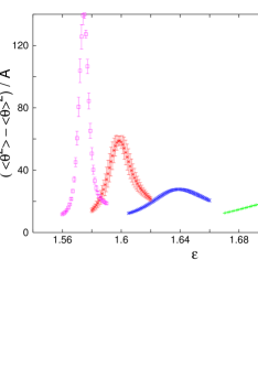
Figure 1: The susceptibility $\chi_{ext}$ in $D=3$ dimensions

2.1 Numerical results

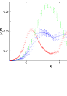
Figure 2: The distribution of the average external curvature $\bar{\Theta}$ in $D=3$ dimensions obtained with re-weighting. The non zero probability for unphysical negative values $\bar{\Theta}<0$ is an artifact of the extrapolation to this region in the re-weighting process.

To localize possible transitions we measure the energy fluctuation of the external curvature field

$$\chi_{ext}=\frac{1}{A}\frac{\partial^{2}}{\partial^{2}\epsilon}\log Z(A,\epsilon)=\frac{<\Theta^{2}>-<\Theta>^{2}}{A}$$ (7)

and search for maxima in this observable. The average external curvature is proportional to the first derivative of the free energy :

$$<\Theta>=\frac{\pi}{2A}\frac{\partial}{\partial\epsilon}\log Z(A,\epsilon)=\frac{1}{2A}\sum_{S}\sum_{l}\Theta_{l}e^{-S[E]}.$$ (8)

We simulated in three and four embedding dimensions and scanned the coupling range $0\leq\epsilon\leq 3$ for maxima of $\chi_{ext}$. In both cases we found a single peak. We used re-weighting methods [10] to extract the shape of the peaks shown in figure 1 from four independent measurements per volume at $\epsilon\approx\epsilon_{pc}$ in $d=3$.

The peaks grow quickly, in fact a bit faster than linear, with the volume. This suggests a first order phase transition, which is confirmed by a look at the distribution of external curvature $\bar{\Theta}$, where the bar indicates the average taken over a given lattice. In figure 2 we show this distribution for $D=3$ and the coupling $\epsilon\approx\epsilon_{pc}$ close to the pseudo-critical coupling. One observes a clear signal of a first order phase transition, namely two maxima separated by a minimum which becomes deeper as the size of the surfaces is increased. This clearly indicates two separate phases. In one phase the average external curvature is close to zero, the typical surface is flat.

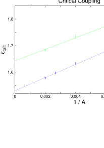
Figure 3: The pseudo-critical coupling $\epsilon_{crit}(1/A)$.

To estimate the critical coupling we use that for a first order phase transition one can expect

$$\epsilon_{pc}(A)=\epsilon_{c}+\frac{c}{A}+O(\frac{1}{A^{2}})$$ (9)

for the scaling of the pseudo-critical couplings $\epsilon_{pc}$. In figure 3 we show the numerical estimates for $\epsilon_{pc}$. Note that the pseudo critical coupling decreases with the volume which indicates that $\epsilon_{c}$ is finite in the thermodynamic limit. With a linear fit to equation (9) we find for the critical coupling

$$\begin{array}[]{cc}D=3&\epsilon_{c}=1.530(3)\\ D=4&\epsilon_{c}=1.643(4)\end{array}.$$

Figure 4: The schematic phase diagram for the Hyper-cubic random surface model with extrinsic curvature. One finds qualitatively the same behavior in $D=3$ and $D=4$ embedding dimensions.

To demonstrate the change in the geometrical behavior we consider the radius of gyration

$$G^{2}(A,\epsilon)=<\frac{1}{A}\sum_{p}(S_{\mu}(p)-S_{\mu}(p_{0}))^{2}>,$$ (10)

which is the average squared distance of the plaquettes to some reference plaquette $p_{0}$. The $S_{\mu}$ are the coordinates of the plquette in the embedding space. In the numerical simulations we do a stochastic average over the $p_{0}$ by choosing 10 % of the plaquettes at random as $p_{0}$ per measurement. One can use the radius of gyration to define the external Haussdorff dimension $d_{h}$

$$G^{2}(A,\epsilon)\approx A^{2/d_{h}}.$$ (11)

In a sense the Haussdorff dimension is the largest possible dimension for the embedding space which can still be completely filled by the surface. We have measured numerically the radius of gyration for $\epsilon=0$ and $\epsilon=2$ for volumes $A$ in the range $200$ to $5000$. With a fit to (11) we extract the Haussdorff dimension:

$$\begin{array}[]{cc}\epsilon=0.&d_{h}=4.07(3)\\ \epsilon=2.&d_{h}=2.00(3).\end{array}$$

The value found for $\epsilon=0$ is two standard deviations away from the expected result [4] but this should presumably be attributed to finite size effects.

The results are summarized in the phase diagram figure 4. The model is defined only for $\mu>\mu_{c}(\epsilon)$ which defines the critical line depicted by the solid line in the phase diagram. Above this line we find two phases. For $\epsilon<\epsilon_{crit}$ the system is in the branched polymer phase with $d_{h}\approx 4$. If we assume hyperscaling

$$\nu=d_{H}^{-1},\quad\gamma=\nu(2-\eta)$$ (12)

the anomalous scaling dimension is $\eta=0$ as expected for a branched polymer. The strong coupling phase is flat, which is reflected by the observation $d_{h}=2$. In this phase basically no baby universes are present. For example, on a surface of size $A=500$ we found at $\epsilon=2$ on average only $0.06$ baby universes of size $B=5$. The largest one found in this phase is of size $33$ and appeared only once in $200000$ measurements. For comparison in the branched polymer phase at $\epsilon=0$ we found in average $10.6$ baby universes of size $5$ on the surface, the probability for the largest possible one with $B=249$ is about $0.02$. Therefore one cannot use the baby universe distribution to measure $\gamma$ in the flat phase. However the fact that there effectively are no baby surfaces means that $\gamma$ is large negative. Therefore the existence of this phase is not in contradiction with [3] because the assumptions (1) are not met.

3 Summary

We have analyzed the model of hypercubic random surfaces with an extrinsic curvature term in the action. We observed a first order phase transition, which separates a branched polymer phase from a flat phase. We have shown that the critical coupling is finite in the thermodynamic limit, i.e. the flat phase survives in the large volume limit and we observe true long-range order. This may seem a bit surprising first because long range correlations in two dimensional systems are rather unusual. In a comparable model of triangulated fluid membranes the existence of a stable, long range ordered phase had somewhat been disputed [11].

Our hope to find a non-trivial, positive $\gamma$ for the geometry at the transition of the external-curvature “field” was not satisfied. Although we find a phase transition, we do not have the situation where the exponent $\overline{\gamma}$ of the individual branches is negative while the exponent for the overall geometry is positive but different from the generic branched polymer value $\gamma=\frac{1}{2}$. Instead we find $\gamma$ large negative, which is also the reason why the transition is not in contradiction with the statement “no transition at finite coupling” for this model given in [3], because this argument relies on the assumption, that $\gamma$ is positive.

References

- [1] D. Weingarten, Phys. Lett. B90 (1080) 280.
- [2] B. Durhuus, J. Fröhlich, T. Johnsson, Nucl. Phys. B240 (1980) 453
- [3] B. Durhuus, T. Jonsson Phys. Lett. B140 (1986) 385.
-
[4]
B. Baumann, B. Berg, Phys. Lett. B164 (1985) 131
B. Baumann, B. Berg, G. Münster, Nucl. Phys. B305 (1988) - [5] B. Durhuus, Nucl. Phys. B426 (1994) 203.
- [6] J. Ambjørn, Nucl. Phys. Proc. Suppl. 42 (1995) 3.
- [7] S. Bilke, Z. Burda, B. Petersson, Phys. Lett. B409 (1997), 173
- [8] V. Knizhnik, A. Polyakov, A. Zamolodchikov, Mod. Phys. Lett. A3 (1988) 819
- [9] S. Bilke, “Studies in Random Geometries: Hypercubic Random Surfaces and Simplicial Quantum Gravity”, PhD-Thesis, hep-lat/9805006
- [10] A.M. Ferrenberg, R.H. Swendsen, Phys. Rev. Lett. 61 (1988) 2635.
-
[11]
J. Ambjørn, A. Irbäck, J. Jurkiewicz, B. Petersson,
Nucl.Phys. B393 (1993) 571
M. Bowick, P. Coddington, L. Han, G. Harris, E. Marinari, Nucl.Phys. B394 (1993) 791
K. Anagnostopoulos, M. Bowick, P. Coddington, M. Falcioni, L. Han, G. Harris, E. Marinari, Phys. Lett.B317 (1993) 102