We construct and test a quasi-perfect lattice action for staggered fermions. The construction starts from free fermions, where we suggest a new blocking scheme, which leads to excellent locality of the perfect action. An adequate truncation preserves a high quality of the free action. An Abelian gauge field is inserted in $d=2$ by effectively tuning the couplings to a few short-ranged lattice paths, based on the behavior of topological zero modes. We simulate the Schwinger model with this action, applying a new variant of Hybrid Monte Carlo, which damps the computational overhead due to the non-standard couplings. We obtain a tiny “pion” mass down to very small $\beta$, while the “$\eta$” mass follows very closely the prediction of asymptotic scaling. The observation that even short-ranged quasi-perfect actions can yield strong improvement is most relevant in view of QCD.

1 Introduction

Most QCD simulations so far have been performed either using Wilson fermions [1] or staggered fermions [2]. The latter formulation is especially useful in the chiral limit, because the remnant chiral symmetry $U(1)\otimes U(1)$ protects the zero fermion mass from renormalization. As a related virtue, its artifacts due to the lattice spacing $a$ are only of $O(a^{2})$, whereas they are of $O(a)$ for Wilson fermions interacting by gauge fields.

It is now widely accepted that the above lattice actions should be improved, so that the lattice spacing artifacts are suppressed and coarser lattices can be used [3]. There are essentially two improvement strategies in the literature. In Symanzik’s program [4] the action is improved in orders of $a$. For QCD with Wilson fermions this has been realized on-shell to the first order on the classical level [5] and recently also on the quantum level [6]. Less work has been devoted to the improvement of staggered fermions, perhaps because the artifacts in the standard formulation are already smaller. However, S. Naik has applied Symanzik’s program on-shell, where he improved the free staggered fermion by adding more couplings along the axes [7], and the Bielefeld group did the same by adding diagonal couplings [8]. Furthermore, the MILC collaboration achieved a reduced pion mass by treating the gauge variable as a “fat link” [9]. Finally, some work on improved operators has been done in this framework [10].

The other promising improvement scheme is non-perturbative in $a$ and uses renormalization group concepts. It has been known for a long time that there are perfect lattice actions in parameter space, i.e. actions without any cutoff artifacts [11]. More recently, it has been suggested to approximate them for asymptotically free theories as “classically perfect actions” [12], which works very well in a number of two dimensional models [12, 13, 14, 15], and it has also been applied in 4d pure Yang-Mills gauge theory [16, 17].

For free or perturbatively interacting fields, perfect actions can be constructed analytically in momentum space. For Wilson type fermions this has been carried out to the first order in the gauge coupling in the Schwinger model [18] and in QCD [19]. A technique called “blocking from the continuum” was extremely useful for this purpose. One expresses all quantities in lattice units after the blocking, and sends the blocking factor to infinity. Hence the blocking process starts from a continuum theory, and it does not need to be iterated in order to identify a perfect action.

For staggered fermions, a block variable renormalization group transformation (RGT), which does not mix the pseudo flavors and which does therefore preserve the important symmetries, has been suggested in Ref. [20]. It requires an odd blocking factor $n$. Iterating the $n=3$ block variable RGT, a fixed point action, i.e. a perfect action at infinite correlation length, has been constructed [13, 21]. Also for staggered fermions blocking from the continuum is applicable [22]. This has been carried out for a general (flavor non-degenerate) mass term, revealing the intimate relation to the Dirac-Kähler fermion formulation in the continuum [23], and also including a suitable treatment of the gauge field [24]. Using the generalization to a flavor non-degenerate mass [23], the spectral doublers inherent to the staggered fermion formulation might be treated as physical flavors in a QCD simulation.

In the present paper, first the procedure of blocking staggered fermions from the continuum is revisited. We then discuss the optimization of locality, in the sense of an extremely fast exponential decay of the couplings in coordinate space. This property is crucial for practical applications, because we have to truncate the couplings to a small number, which is tractable in simulations. Of course the truncation violates the perfectness, but for excellent locality this violation is not too harmful.

We suggest a new blocking scheme, which we call “partial decimation”. It leads to a higher degree of locality than the usual block average method, i.e. to a faster exponential decay of the couplings in coordinate space. We then truncate the couplings to a short range by means of mixed periodic and anti-periodic boundary conditions, which are particularly adequate for staggered fermions. The excellent quality of the truncated perfect action for free staggered fermions is confirmed by spectral and thermodynamic considerations.

We then proceed to the two flavor Schwinger model [25] as a test case. The Schwinger model is well-understood from continuum calculations, also in finite volume [26, 27, 28]. It shares important features with QCD, such as asymptotic freedom, confinement and topological quantum numbers with corresponding zero-modes of the Dirac operator. On the other hand, one expects other features of higher-dimensional gauge theories not to be well-represented by the Schwinger model, due to its super-renormalizability.

The fermion gauge vertex is added “by hand” to the truncated perfect free fermion. We first insert the $U(1)$ links between fermionic source and sink along certain shortest lattice paths. In a second step, we implement “fat links” for the paths consisting of just one link. The staple weight is determined effectively by minimizing the eigenvalues of the approximate topological zero-modes. For the pure gauge part, we use two actions, which are perfect resp. approximately perfect in $d=2$.

Of course, the ad hoc treatment of the vertex deviates from the systematic construction of a (classically) perfect action. However, in the staggered scheme any approximation or truncation of perfect action can cause errors of $O(a^{2})$ at most, and the remnant axial symmetry protects the mass term from renormalization. By contrast, a strong mass renormalization is a severe problem for quasi-perfect fermions of the Wilson type [29, 30, 31, 32].

Naively, the computational effort for simulations increases about linearly with the number of couplings in the action. In addition, physical effects, e.g. more exact zero-modes, may be a hurdle for the application of an improved action. We propose a way to damp this increase of computational costs, exploiting the freedom to design the Molecular Dynamic steps in the Hybrid Monte Carlo algorithm. We use a simplified action there, and the full quasi-perfect action in the Metropolis acceptance decision. We discuss the performance of this method for different values of $\beta$, the crucial question being the acceptance rate. This method may also accelerate simulations with improved actions on parallel machines. It depends on a sufficiently good simplified version of the improved action, which is another plus for staggered fermions.

For quasi-perfect staggered fermions, the dispersion relation and the scaling behavior of the mass spectrum are good down to $\beta$ $\stackrel{{\scriptstyle<}}{{\sim}}$ 1.5. For these low values of $\beta$, the masses for the $\pi$- and $\eta$-particle demonstrate a good scaling resp. asymptotic scaling behavior. In particular the scaling is even better than the one observed in Ref. [15], which uses truncated perfect Wilson type fermions, and 123 independent couplings parameterizing a classically perfect fermion-gauge vertex. Compared to that scheme, a drastically reduced number of couplings is needed here, and even more in the step to $d=4$. Our results demonstrate that in fact a relatively modest number of couplings can yield a very powerful improvement.

A synopsis of this work was presented in Ref. [33].

2 The staggered blocking scheme

The construction of perfect actions for free staggered fermions by blocking from the continu-um has been described in Refs. [23, 24]. We start by briefly reviewing this procedure. The staggered blockspin fermions are defined in two steps. First we transform the $N_{f}=2^{d/2}$ flavors of continuum Dirac spinors $\psi_{a}^{b}(x)$ ($a$: spinor index, $b$: flavor index) into the Dirac-Kähler (DK) representation given by $\varphi(x,H)$. These functions originate from the representation of inhomogeneous differential forms

$$\sum_{H}\varphi(x,H)\,dx^{H}\ ,\ \ dx^{H}\ =\ dx^{\mu_{1}}\wedge\dots\wedge dx^{\mu_{h}}\ ,$$ (2.1)

where $H=\{\mu_{1},\dots,\mu_{h}\},\ \mu_{1}<\dots<\mu_{h}$ is a multi-index. Transformation and inverse transformation read

$$\varphi(x,H) = \frac{1}{\sqrt{N_{f}}}\sum_{ab}\left.\gamma^{H}_{ab}\right.^{*}\,\psi_{a}^{b}(x)\ ,\ \ \ \gamma^{H}\ =\ \gamma^{\mu_{1}}\gamma^{\mu_{2}}\dots\gamma^{\mu_{h}}\ ,$$ (2.2)

$$\psi_{a}^{b}(x) = \frac{1}{\sqrt{N_{f}}}\sum_{H}\gamma^{H}_{ab}\,\varphi(x,H)\ .$$ (2.3)

Second, we introduce a coarse lattice of double unit spacing $\bar{\Gamma}=\{\bar{y}\,|\,\bar{y}_{\mu}=2\bar{n}_{\mu}\}$, which is a sublattice of $\Gamma=\{y\,|\,y_{\mu}=n_{\mu}\}$, with $\bar{n}_{\mu},n_{\mu}\in Z\!\!\!Z$. The fine lattice points $y$ are uniquely decomposed as ($\hat{\mu}$ is the unit vector in $\mu$–direction)

$$y\ =\ \bar{y}\,+\,e_{H}\ ,\ \ e_{H}\ =\ \sum_{\mu\in H}\hat{\mu}\ .$$ (2.4)

Thus the multi-index $H(y)$ defines the position of a fine lattice point $y$ with respect to the coarse lattice $\bar{\Gamma}$. Now the blockspin variables $\Psi(y)$ can be defined as averages of the component functions $\varphi(x,H(y))$, with a normalized weight $\Pi(x\!-\!y)$, $\int\!dx\,\Pi(x\!-\!y)=1$, which is assumed to be even and peaked around $x=y$,

$$\Psi(y)\ =\ \frac{1}{\sqrt{N_{f}}}\sum_{ab}\left.\gamma^{H(y)}_{ab}\right.^{*}\,\int dx\ \Pi(x-y)\ \psi_{a}^{b}(x)\ .$$ (2.5)

This scheme has been proposed first in Ref. [22]. Its peculiarity is that the staggered block centers depend on the multi-index $H$ of the Dirac-Kähler component functions $\varphi(x,H)$. Block average (BA) means in this case average over the overlapping lattice hypercubes $[y]=\{x|-1\leq(x_{\mu}-y_{\mu})\leq 1\}$. This scheme is given by $\Pi=\Pi_{BA}$, $\Pi_{BA}(x)=2^{-d}$ for $x\in[y]$, and $\Pi_{BA}(x)=0$ otherwise.

For the following calculation we diagonalize the lattice action using the staggered symmetries. Here it is important that fine lattice shifts are no symmetry transformations. However, combination with site-dependent sign factors gives rise to the non-commuting flavor symmetry transformations [36]. Therefore we replace ordinary Fourier transformation by harmonic analysis with respect to flavor transformations and coarse lattice translations. We thus obtain a modified momentum representation which intertwines Fourier transformation and the transition back from DK fermions to the Dirac basis,

$$\Psi_{a}^{b}(p) = \sum_{y}\,e^{ipy}\,\gamma^{H(y)}_{ab}\,\Psi(y)\ ,$$

$$\bar{\Psi}_{a}^{b}(p) = \sum_{y}\,e^{ipy}\,\gamma^{H(y)}_{ab}\,\bar{\Psi}(y)\ ,\qquad p\in{\cal B}\ =\ ]-\pi/2,\pi/2]^{d}$$ (2.6)

(${\cal B}$ is the Brillouin zone with respect to the coarse lattice). Inserting Eq. (2.5) we find

$$\Psi_{a}^{b}(p)\ =\ \frac{1}{\sqrt{N_{f}}}\int\frac{dp^{\prime}}{\pi^{d}}\sum_{a^{\prime}b^{\prime}}\ \Pi(p^{\prime})\ \psi_{a^{\prime}}^{b^{\prime}}(p^{\prime})\ \sum_{y}\ e^{i(p-p^{\prime})y}\ \gamma^{H(y)}_{ab}\left.\gamma^{H(y)}_{a^{\prime}b^{\prime}}\right.^{*}\ ,$$ (2.7)

where $\psi_{a}^{b}(p),\Pi(p)$ denote the Fourier transforms of $\psi_{a}^{b}(x),\Pi(x)$. The last sum can be re-written as

$$\sum_{\bar{y}\in\bar{\Gamma}}\,e^{iq\bar{y}}\ \sum_{K}e^{iqe_{K}}\ \gamma^{K}_{ab}\left.\gamma^{K}_{a^{\prime}b^{\prime}}\right.^{*} = \pi^{d}\sum_{l\in Z\!\!\!Z^{d}}\delta(q-\pi l)\ \sum_{K}\prod_{\mu\in K}(-1)^{l_{\mu}}\ \gamma^{K}_{ab}\left.\gamma^{K}_{a^{\prime}b^{\prime}}\right.^{*}$$ (2.8)

$$= N_{f}\,\pi^{d}\sum_{l\in Z\!\!\!Z^{d}}\delta(q-\pi l)\ \gamma^{\hat{H}(l)}_{aa^{\prime}}\left.\gamma^{\hat{H}(l)}_{b^{\prime}b}\right.^{\dagger}\ .$$

We have used the orthogonality of the $\gamma$–matrix elements

$$\sum_{H}\gamma^{H}_{ab}\,\left.\gamma^{H}_{a^{\prime}b^{\prime}}\right.^{*}\ =\ N_{f}\ \delta_{aa^{\prime}}\,\delta_{bb^{\prime}}\ ,$$ (2.9)

and $\hat{H}(l)$ is defined by $H(l)=\{\mu\,|\,l_{\mu}\,\mbox{is odd}\}$, $\hat{H}=H$ for $h$ even, $\hat{H}=\{\mu\,|\,\mu\not\in H\}$ for $h$ odd. Finally Eq. (2.7) becomes (summation over double spin and flavor indices is understood)

$$\Psi_{a}^{b}(p)=\sqrt{N_{f}}\ \sum_{l\in Z\!\!\!Z^{d}}\ \Pi(p+\pi l)\ \hat{\psi}_{a}^{b}(p+\pi l)\ ,\ \hat{\psi}_{a}^{b}(p+\pi l)=\gamma^{\hat{H}(l)}_{aa^{\prime}}\ \psi_{a^{\prime}}^{b^{\prime}}(p+\pi l)\ \left.\gamma^{\hat{H}(l)}_{b^{\prime}b}\right.^{\dagger}.$$ (2.10)

Note that the blockspin transformation is diagonal with respect to spin and flavor for continuum momenta within the first Brillouin zone ${\cal B}$, yet not for all $l\neq 0$.

We are now prepared to compute the perfect action for a RGT of the Gaussian type. Starting from a continuum action with a general mass term $m_{b}$ – which does not need to be flavor degenerate – the perfect lattice action $S[\bar{\Psi},\Psi]$ is defined as

$$e^{-S[\bar{\Psi},\Psi]}\ =\ \int\!{\cal D}\bar{\psi}{\cal D}\psi\int\!{\cal D}\bar{\eta}{\cal D}\eta\ \ \exp\Bigl{\{}-\int\!\!\frac{dq}{N_{f}\,\pi^{d}}\ \bar{\psi}_{a}^{b}(-q)\left(i\gamma^{\mu}_{aa^{\prime}}q_{\mu}+m_{b}\right)\psi_{a^{\prime}}^{b}(q)\Bigr{\}}$$ (2.11)

$$\times \exp\Bigl{\{}\int_{{\cal B}}\frac{dp}{N_{f}\,\pi^{d}}\ \Bigl{[}\ [\bar{\Psi}_{a}^{b}(-p)\,-\,\sqrt{N_{f}}\sum_{l\in Z\!\!\!Z^{d}}\Pi(p+\pi l)\ \hat{\bar{\psi}}_{a}{}^{b}(-p-\pi l)\ ]\ \eta_{a}^{b}(p)$$

$$+\bar{\eta}_{a}^{b}(-p)\ [\ \Psi_{a}^{b}(p)\,-\,\sqrt{N_{f}}\sum_{l\in Z\!\!\!Z^{d}}\Pi(p+\pi l)\ \hat{\psi}_{a}{}^{b}(p+\pi l)\ ]$$

$$+\bar{\eta}_{a}^{b}(-p)D_{aa^{\prime}}^{b}(p)\eta_{a^{\prime}}^{b}(p)\Bigr{]}\Bigr{\}}\ ,$$

where $\bar{\eta}$, $\eta$ are auxiliary Grassmann fields defined on the same sites and with the same flavor structure as $\bar{\Psi}$, $\Psi$. A non-zero term

$$D_{aa^{\prime}}^{b}(p)\ =\ \gamma^{\mu}_{aa^{\prime}}D_{\mu}^{b}(p)\ +\ \delta_{aa^{\prime}}\,D_{0}^{b}(p)$$ (2.12)

“smears out” the blockspin transformation, as in Ref. [24]. This term is used to optimize locality of the resulting perfect action; it will be specified later on. The Gaussian integrals over $\psi$,$\bar{\psi}$ and $\bar{\eta}$,$\eta$ can be evaluated by substitution of the classical fields, which leads to

$$S[\bar{\Psi},\Psi]\ =\ \int_{{\cal B}}\frac{dp}{N_{f}\,\pi^{d}}\ \Bigl{[}\ \bar{\Psi}_{a}^{b}(-p)\ G^{-1}{}_{aa^{\prime}}^{bb^{\prime}}(p)\ \Psi_{a^{\prime}}^{b^{\prime}}(p)\ \Bigr{]}\ ,$$ (2.13)

with the lattice propagator

$$G_{aa^{\prime}}^{bb^{\prime}}(p)\,=\,D_{aa^{\prime}}^{bb^{\prime}}(p)\,+\,\sum_{l\in Z\!\!\!Z^{d}}\Bigl{(}\Pi(p+\pi l)^{2}\,\gamma^{\hat{H}(l)}_{bd}\ \frac{[-i(-1)^{k_{\nu}}\gamma^{\mu}_{aa^{\prime}}(p+\pi l)_{\mu}+m_{d}]\,\delta_{dd^{\prime}}}{(p+\pi l)^{2}+m_{d}^{2}}\left.\gamma^{\hat{H}(l)}_{d^{\prime}b^{\prime}}\right.^{\dagger}\Bigr{)}\ .$$ (2.14)

Note that $G$ is flavor diagonal, $G^{bb^{\prime}}=G^{b}\delta^{bb^{\prime}}$, because $\gamma^{\hat{H}(l)}\gamma^{K}\left.\gamma^{\hat{H}(l)}\right.^{\dagger}$ is diagonal iff $\gamma^{K}$ is. In particular, for a degenerate mass term the adjungation with $\gamma^{\hat{H}(l)}$ is trivial, and the lattice propagator is proportional to $\delta_{bb^{\prime}}$ in flavor space. We define

$$G^{b}_{aa^{\prime}}(p)\ =\ -i\sum_{\mu}\gamma^{\mu}_{aa^{\prime}}\,Q^{b}_{\mu}(p)\ +\ \delta_{aa^{\prime}}Q^{b}_{0}(p)\ ,$$ (2.15)

hence $Q_{\mu}^{b},Q_{0}^{b}$ become

$$Q^{b}_{\mu}(p) = D_{\mu}^{b}(p)\,+\sum_{l\in Z\!\!\!Z^{d}}\Pi(p+\pi l)^{2}\frac{1}{N_{f}}\sum_{b^{\prime}}\sum_{K}\epsilon_{K}(l)\,\gamma^{K}_{bb}\left.\gamma^{K}_{b^{\prime}b^{\prime}}\right.^{*}\frac{(-1)^{l_{\mu}}(p+\pi l)_{\mu}}{(p+\pi l)^{2}+m_{b^{\prime}}^{2}}\,,\qquad$$ (2.16)

$$Q^{b}_{0}(p) = D_{0}^{b}(p)\,+\sum_{l\in Z\!\!\!Z^{d}}\Pi(p+\pi l)^{2}\frac{1}{N_{f}}\sum_{b^{\prime}}\sum_{K}\epsilon_{K}(l)\,\gamma^{K}_{bb}\left.\gamma^{K}_{b^{\prime}b^{\prime}}\right.^{*}\frac{m_{b^{\prime}}}{(p+\pi l)^{2}+m_{b^{\prime}}^{2}}\,.\qquad$$ (2.17)

In case of a non-degenerate mass $m_{b}$ the sums $\sum_{b^{\prime}}\sum_{K}$ cannot be contracted according to Eq. (2.9), due to the sign factor $\epsilon_{K}(l)=\prod_{\nu\in K}(-1)^{l_{\nu}}$. However, in the degenerate case $m_{b}=m$, with flavor independent smearing terms $D^{b}=D$, we simply obtain

$$Q_{\mu}(p) = D_{\mu}(p)\ +\ \sum_{l\in Z\!\!\!Z^{d}}\Pi(p+\pi l)^{2}\,\frac{(-1)^{l_{\mu}}(p+\pi l)_{\mu}}{(p+\pi l)^{2}+m^{2}}\ ,$$ (2.18)

$$Q_{0}(p) = D_{0}(p)\ +\ \sum_{l\in Z\!\!\!Z^{d}}\Pi(p+\pi l)^{2}\frac{m}{(p+\pi l)^{2}+m^{2}}\ .$$ (2.19)

The perfect action in real space arises from Eq. (2.13) inserting the momentum representation given in Eq. (2.6). After some $\gamma$–matrix algebra [23], we arrive at

$$S[\bar{\Psi},\Psi] = \sum_{y,y^{\prime}}\bar{\Psi}(y)\,{\bf m}(y,y^{\prime})\,\Psi(y^{\prime})\ ,$$ (2.20)

$${\bf m}(y,y^{\prime}) = \sum_{K}\rho^{K}(y^{\prime})\rho(y-y^{\prime},y^{\prime})\ M^{K}(y-y^{\prime})\ .$$ (2.21)

Corresponding to a lattice propagator diagonal in flavor space, the sum over $K$ runs over multi-indices $K\in{\cal D}$ with diagonal $\gamma^{K}$, in the Weyl basis ${\cal D}\,=\,\{\emptyset,\ 1\,2,\ 3\,4,\ 1\,2\,3\,4\}$. The sign factors $\rho(z,y)\equiv\rho(H(z),H(y))$ arise from $\gamma^{H}\gamma^{K}=\rho(H,K)\,\gamma^{H\Delta K}$, where $H\Delta K=(H\cup K)\backslash(H\cap K)$, and $\rho^{K}(y)$ is given by $\rho(H(y),K)\rho(K,H(y))$. By symmetry, the only non-zero contributions to $M^{K}(y)$ are

$$M^{K}_{\mu}(y) = i\rho(\mu,K)\int_{{\cal B}}\frac{dp}{\pi^{d}}\ e^{-ipy}\ M^{K}_{\mu}(p)\qquad\mbox{ for }H(y)=\mu\Delta K\ ,\qquad$$ (2.22)

$$M^{K}_{0}(y) = \int_{{\cal B}}\frac{dp}{\pi^{d}}\ e^{-ipy}\ M^{K}_{0}(p)\qquad\qquad\qquad\mbox{ for }H(y)=K\ ,\qquad$$ (2.23)

$$\mbox{with}\quad M^{K}_{\mu,0}(p) = \frac{1}{N_{f}}\sum_{b}\left.\gamma^{K}_{bb}\right.^{*}\,\frac{Q_{\mu,0}^{b}(p)}{\sum_{\nu}Q_{\nu}^{b}(p)^{2}+Q_{0}^{b}(p)^{2}}\ .\qquad$$ (2.24)

The flavor degenerate case leads to vanishing components for $K\neq\emptyset$, and (with $M^{\emptyset}_{\mu,0}=M_{\mu,0}$) we simply obtain

$$M_{\mu,0}(p)\ =\ \frac{Q_{\mu,0}(p)}{\sum_{\nu}Q_{\nu}(p)^{2}+Q_{0}(p)^{2}}\ .$$ (2.25)

It has been proven in Ref. [23] that the couplings given by the fermion matrix ${\bf m}(y,y^{\prime})$ are local, i.e. they decay faster than any power of $|y-y^{\prime}|$. For that, certain periodicity properties apply, which translate into (for simplicity of notion, $\tilde{\mu}$ denotes either $\mu$ or $0$, and $K\Delta 0\equiv K$)

$$Q^{b}_{\tilde{\mu}}(p)\ =\ \sum_{K\in{\cal D}}\gamma^{K}_{bb}\ Q^{K}_{\tilde{\mu}}(p)\ ,\quad Q^{K}_{\tilde{\mu}}(p+\pi\hat{\nu})\ =\ \left\{\begin{array}[]{ll}-Q^{K}_{\tilde{\mu}}(p)&\mbox{ for }\nu\,\in\ K\Delta\tilde{\mu}\\ Q^{K}_{\tilde{\mu}}(p)&\mbox{ for }\nu\,\not\in\ K\Delta\tilde{\mu}\end{array}\right.\ .$$ (2.26)

Again, we sum over diagonal $\gamma$–matrices only. It is provided that the corresponding requirements are met for the smearing terms $D^{b}_{\tilde{\mu}(p)}$ within $Q^{b}_{\tilde{\mu}}(p)$, see below. In consequence, the fermion matrix components $M^{K}_{\tilde{\mu}}(p)$ obey periodicity conditions analogous to $Q^{K}_{\tilde{\mu}}(p)$, and the integrands of Eqs. (2.22, 2.23) are periodic with respect to the Brillouin zone ${\cal B}$ and analytic in a strip around the real axis. This implies locality of the perfect action.

The coupling of even and odd lattice points is due to the $M^{K}_{\mu}$ components of the fermion matrix; the $M^{K}_{0}$ components couple even–even and odd–odd. We add without proof that even-odd decoupling of the Hermitian matrix ${\bf m}^{\dagger}\,{\bf m}$ can be shown in any even dimension $d$ with arbitrary (non-degenerate) mass terms for truncated versions of the perfect fermion matrix ${\bf m}(y,y^{\prime})$, see Ref. [23] for $d=2$. This is a useful property in simulations with Hybrid Monte Carlo algorithms. However, with (non-perfect) coupling to a gauge field and non-zero mass term (i.e. with even–even, odd–odd as well as even–odd couplings), this is not true in general.

3 Optimization of locality

In the blocking scheme described so far, there is quite some freedom left. In particular, we may use averaging functions different from $\Pi_{BA}$, and we can choose the smearing term $D$ in Eq. (2.11). In both cases we aim at optimization of the locality in the resulting perfect action.

Let us first discuss the averaging scheme. In Eq. (2.11) we implicitly assumed the same blocking of $\psi$ and $\bar{\psi}$, given by the weight function $\Pi(x)$ resp. its Fourier transform $\Pi(p)$. Now we consider the case of a block average $\Pi=\Pi_{BA}$ for $\psi$ ($\bar{\psi}$) only, while $\bar{\psi}$ ($\psi$) is put on the lattice by decimation, $\Pi(x)=\delta(x)$. Thus we obtain a single factor $\Pi(p+\pi l)$ in Eq. (2.14) with

$$\Pi(p)\ =\ \Pi_{BA}(p)\ =\ \prod_{\mu}\frac{\hat{p}_{\mu}}{p_{\mu}}\ ,\qquad\hat{p}_{\mu}\ =\ \sin p_{\mu}\ .$$ (3.1)

In case of a $\delta$ function RGT ($D=0$), this means to identify the averaged continuum and lattice 2-point functions

$$\langle\ \phi(y)\ \bar{\phi}(y^{\prime})\ \rangle\ =\ \int_{[y]}dx\ \langle\ \varphi(x,H(y))\ \bar{\varphi}(y^{\prime},H(y^{\prime}))\ \rangle\ .$$ (3.2)

Due to translation invariance it does not matter whether we average source or sink of the continuum expression, or whether we allocate the space directions to be integrated over to source and sink in some way. (The last point of view may be used to make a closer contact to the construction of staggered fermions from DK fermions in the continuum [35], as discussed in Ref. [23].) We call this blocking scheme partial decimation. For the 2-point functions every space direction is integrated over once; therefore we do not run into the difficulties arising for blockspin transformations with complete decimation, which do not have a corresponding perfect action.

For both blocking schemes, block average for $\psi$ and $\bar{\psi}$ (BA) and partial decimation (PD), we now want to optimize locality of the couplings by making use of the smearing terms in Eqs. (2.16, 2.17). As an optimization criterion it has been suggested to require that in the effectively 1d case – with momenta $p=(p_{1},0,\dots,0)$ – the couplings are restricted to nearest neighbors as in the standard action [19, 21]. In the degenerate case we require

$$i\gamma_{1}\,M_{1}(p_{1},0,\dots,0)\ +\ M_{0}(p_{1},0,\dots,0)\ =\ f(m)\,[\,i\hat{p}_{1}\,\gamma_{1}\ +\ \hat{m}\,],$$ (3.3)

with $\hat{m}|_{m=0}=0$ and $f(0)=1$. Our ansatz for the Gaussian smearing term reads

$$D_{\mu}(p)=c(m)\hat{p}_{\mu},\qquad D_{0}(p)=a(m).$$ (3.4)

Requirement (3.3) can be fulfilled in both blocking schemes we are considering, if we specify the RGT as follows

$$c_{BA}(m) = [\cosh m-1]\,/\,(2m)^{2}\ ,\quad a_{BA}(m)\ =\ [\sinh(2m)-2m]\,/\,(2m)^{2}\ ,$$

$$c_{PD}(m) = 0\ ,\qquad\qquad\qquad\qquad\qquad\!a_{PD}(m)\ =\ [\cosh m-1]\,/\,(2m)\ .$$ (3.5)

In both cases, we obtain $\hat{m}=\sinh m$. For $m=0$ a non-vanishing static smearing term $a(0)$ would explicitly break the remnant chiral symmetry in the fixed point action. Therefore, the static term should vanish for optimized locality, as it does in both cases. Furthermore, in the PD scheme the chiral limit is optimized for locality by a simple $\delta$ function RGT. As an advantage of this property – which is not provided by the BA scheme – there is a direct relation between the $n$-point functions in the continuum and on the lattice. In addition, the extension to interacting theories might involve numerical RGT steps in the classical limit, which also simplify in the absence of a Gaussian smearing term. Finally, a non-vanishing term $c(m)$ causes complications if one wants to include a gauge interaction in the RGT, but the PD scheme avoids such problems.

The decay of the couplings ${\bf m}(x,0)={\bf m}(x)$ in the massless case for $d=2$ and $d=4$ is shown in Figures 1 and 2.

Figure 1: The decay of couplings in (1,0) direction for $d=2$ in the massless case: BA without smearing (diamonds), BA optimized (squares), PD (triangles).

Figure 2: The decay of 4d couplings in various directions in the massless case: BA with optimal smearing term and PD. We see that the latter couplings decay faster.

We see that the PD blocking scheme works better. In the non-degenerate case, the simplest ansatz for a smearing term is (corresponding to the staggered fermion action with non-degenerate mass [38])

$$D^{b}_{\mu}(p)\ =\ c\,\hat{p}_{\mu}\ ,\qquad D^{b}_{0}(p)\ =\ \sum_{K\in{\cal D}}\gamma^{K}_{bb}\ a_{K}\prod_{\mu\in K}\cos p_{\mu}\ .$$ (3.6)

In this case, we obtained – by means of numerical optimization – a similar decay of couplings as with degenerate masses, yet no strict 1-dimensional ultralocality. For $d=2$ it appears that a non-degenerate parameter $a_{12}\neq 0$ does not improve the coupling decay significantly, so we worked with $a_{12}=0$. Again the PD scheme, where we assumed $c_{PD}=0$, leads to a more local action, see Figure 3.

Figure 3: The decay of couplings in (1,0) direction for $d=2$ with masses $m_{1}=0$, $m_{2}=0.5$: BA without smearing (diamonds), BA optimized (squares), PD (triangles).

4 Truncation effects

The litmus test of any perfect action is given by the truncation effects in a practicable number of remaining couplings. These effects are minimized by maximal locality. Yet, the truncation scheme itself may have some impact on the truncation errors. An elegant procedure has been proposed in Ref. [29] for Wilson fermions. First the perfect action is constructed on a small lattice volume $N^{d}$ by restricting the momentum components to the discrete values $p_{\mu}=2\pi n_{\mu}/N\in]-\pi,\pi]$, $n_{\mu}\in Z\!\!\!Z$. Typically, one chooses $N=3$, and the resulting couplings are then used in a large volume too, where they are not exactly perfect any more. This truncation scheme has the virtues of automatically correct normalizations, and a simplification of the numerical evaluation as opposed to a truncation in coordinate space. Furthermore, the mapping to the corresponding truncated perfect action in a lower dimension remains exact; for instance, one can reproduce the effectively 1d nearest neighbor action starting from $d>1$ by summing over the extra dimensions, which provides a sensitive test of the numerical accuracy. Provided a good locality, this method works well for Wilson-type fermions, gauge fields [29] and scalars [37].

For staggered fermions, only a crude truncation in coordinate space has been applied so far [24]. One includes the coupling distances $\pm 1,\ \pm 3$ in the $\mu$ direction, and $2,0,-2$ in the non-$\mu$ directions. This involves more couplings than the $N=3$ truncated Wilson-type fermion (called “hypercube fermion”), whereas the number of degrees of freedom is the same in both cases. However, although significant improvement has been achieved compared to the standard staggered formulation, the quality of its spectral and thermodynamic properties did not reach the level of the “hypercube fermion”. In order to arrive at results of a similar quality, we adapt the above truncation procedure – together with the PD scheme – to the case of staggered fermions.

We treat the components of the fermion matrix $M^{K}_{\tilde{\mu}}(p),\tilde{\mu}=\mu,0$ separately, as they show different behavior under reflections,

$$M^{K}_{\tilde{\mu}}(p_{1}\dots p_{\nu-1},-p_{\nu},p_{\nu+1}\dots p_{d})\ =\ \left\{\begin{array}[]{ll}-M^{K}_{\tilde{\mu}}(p)&\mbox{ for }\nu\,\in\ K\Delta\tilde{\mu}\\ M^{K}_{\tilde{\mu}}(p)&\mbox{ for }\nu\,\not\in\ K\Delta\tilde{\mu}\end{array}\right.\ .$$ (4.1)

Again we use the short-hand notation $K\Delta\tilde{\mu}=K$ for $\tilde{\mu}=0$. Truncation is achieved by discrete Fourier transformation and a discrete support given by $c_{N}(y_{\mu})=1,1/2,0$ for $|y_{\mu}|<,=,>N$, respectively,

$$M^{K}_{\tilde{\mu};N}(y)\ =\ \prod_{\mu}\frac{\pi c_{N}(y_{\mu})}{N}\ \sum_{p\in{\cal B}^{K}_{\tilde{\mu};N}}e^{-ipy}M^{K}_{\tilde{\mu}}(p)\ .$$ (4.2)

It is the set of discrete momenta ${\cal B}^{K}_{\tilde{\mu};N}$ which depends on the reflection properties given by $\tilde{\mu},K$. We choose mixed periodic and antiperiodic boundary conditions,

$$p\in{\cal B}^{K}_{\tilde{\mu};N}\ \Leftrightarrow\ p_{\nu}=\left\{\begin{array}[]{ll}(n+1/2)\pi/N&\mbox{ for }\nu\,\in\ K\Delta\tilde{\mu}\\ n\pi/N&\mbox{ for }\nu\,\not\in\ K\Delta\tilde{\mu}\end{array}\right.,\ n\in Z\!\!\!Z,\ \ p_{\nu}\in\ ]-\pi/2,\pi/2]\ .$$ (4.3)

It is easily verified that the transformation of the truncated components back to momentum space reproduces the perfect values at $p\in{\cal B}^{K}_{\tilde{\mu};N}$ ,

$$M^{K}_{\tilde{\mu};N}(p)\equiv\sum_{y}e^{ipy}\,M^{K}_{\tilde{\mu};N}(y)\ =\ M^{K}_{\tilde{\mu}}(p)\quad\mbox{ for }\ p\in{\cal B}^{K}_{\tilde{\mu};N}\ .$$ (4.4)

The components $M^{K}_{\tilde{\mu}}(y)$ inherit the reflection behavior of $M^{K}_{\tilde{\mu}}(p)$ described in Eq. (4.1). Therefore, treating them as periodic functions in $y$–space by discrete momenta $p_{\nu}=\pi n/N,n\in Z\!\!\!Z$ would make them vanish artificially on the boundaries $y_{\nu}=\pm N$ for $\nu\in K\Delta\tilde{\mu}$. We avoid this defect by the above choice of discrete momenta. It pays off by a drastic reduction of truncation effects, see Figure 4 for the 2d spectrum in the massless case using partial decimation.

Figure 4: The massless spectrum in $d=2$. We compare standard staggered fermions (crosses) and perfect spectrum (full line) with perfect actions truncated with $N=3$ and mixed periodic boundary conditions: block average (dotted), partial decimation (dashed). The last case is also plotted for truncation with periodic boundary conditions (dashed-dotted).

Figure 5: The spectrum in $d=2$ for $m_{1}=0,m_{2}=0.5$. Standard staggered (crosses) and perfect spectrum (full line) are compared with perfect actions truncated with $N=3$ mixed periodic boundary conditions: block average (dotted), partial decimation (dashed).

The values of the perfect couplings, truncated by mixed periodic boundary conditions (as described above) for $N=3$, are given in Table 1.

$d=4$			$d=2$
	PD	BA		PD	BA
(1,0,0,0)	0.348194	0.331558	(1,0)	0.4391168527	0.433150
(1,2,0,0)	0.020490	0.022963	(1,2)	0.0304416413	0.033425
(1,2,2,0)	0.002240	0.002435
(1,2,2,2)	0.000247	0.000180
(3,0,0,0)	0.007609	0.011721	(3,0)	0.0052123698	0.008022
(3,2,0,0)	-0.000216	-0.000319	(3,2)	-0.0026062073	-0.004011
(3,2,2,0)	-0.000384	-0.000605
(3,2,2,2)	-0.000214	-0.000317

Table 1: The couplings of the perfect action for massless staggered fermions, constructed from the “partial decimation” (most successful) and from the optimized “block average” scheme, and truncated by mixed periodic boundary conditions. The couplings are odd in the odd component, and even in all other components. Among the latter there is also permutation symmetry. The 2d PD couplings (given to higher accuracy) are used in the Schwinger model simulation reported below.

Furthermore, the truncation effects are significantly stronger for even truncation distances $N$; in particular, for $N=2$ and $N=4$ the energies become complex-valued at large momenta.

For $N=3$ – which is still tractable in numerical simulations – the amount of improvement is already striking. We compare the spectra for $d$ = 2 in the PD and BA blocking scheme in the massless case (Figure 4) and for non-degenerate masses $m_{1}=0,m_{2}=0.5$ (Figure 5). The couplings derived from the PD blocking scheme turn out to be better, in agreement with the higher degree of locality observed in the (untruncated) perfect action. We see that the improvement is still good in the case of non-degenerate masses. In this case, we optimized the smearing parameters numerically, as pointed out in Section 3. The values are $a_{BA}=0.120$, $c_{BA}=0.125$, $a_{PD}=0.082$, $c_{PD}=0$. The standard staggered fermion results for non-degenerate masses are calculated with the action proposed in Ref. [38]. We emphasize that the spectra of (untruncated) perfect actions are indeed perfect, i.e. identical to the continuum spectra (up to periodicity, which is inevitable on the lattice). Hence the spectrum reveals directly the artifacts due to truncation.

Figure 6 compares the massless spectra in $d=4$, and we see that the qualitative behavior observed in $d=2$ persists. We compare the standard staggered fermion, and the optimized BA and PD fixed point fermions, both truncated by $N=3$ mixed periodic boundary conditions. We see again that the PD scheme is superior. Furthermore, we show for comparison also the dispersion relation of a Symanzik improved action called “p6” from Ref. [8]. Symanzik improvement by additional couplings along the axes (Naik fermion, [7]) only yields a moderate quality [24], but the Bielefeld group suggests a number of actions, where Symanzik improvement is achieved by diagonal couplings. The p6 action is the best variant among them, and also Figure 6 confirms its excellent level of improvement. However, it is not obvious how that formulation can include a general mass term in a subtle way.

Figure 6: The dispersion relation for various types of 4d massless staggered fermions along (1,1,0). We compare the standard action, a Symanzik improved action called “p6” from Ref. [8] and the optimized BA and PD fixed point actions, truncated with mixed periodic boundary conditions.

As a further test in $d=4$, we consider two thermodynamic scaling quantities. The first is the ratio $P/T^{4}$ ($P$: pressure, $T$: temperature). According to the Stefan-Boltzmann law, this ratio is $7\pi^{2}/180$ for massless fermions in the continuum, and a lattice action with many discrete points $N_{t}$ in the temporal direction will asymptotically reproduce that value. However, the speed of convergence, and in particular the behavior at small $N_{t}$, depend on the quality of the action. In contrast to the spectrum, this ratio is not even exact for the fixed point action in Eqs. (2.18, 2.19), because of the “constant factors” that we ignored when performing the functional integral in the RGT Eq. (2.11). Such factors may depend on the temperature, so with respect to thermodynamics our action is not fully renormalized [29]. However, it turns out that the unknown factor is very close to 1, except for the regime of small $N_{t}$ (about $N_{t}\leq 6$), which corresponds to very high temperature. So the main issue is again the contamination due to the truncation.

In Figure 7 we compare this thermodynamic scaling for a variety of staggered fermion actions at $m=0$, and again the PD scheme turns out to be very successful. A similar level of improvement can be observed for the p6 action, which is also here by far better than the Naik fermion. We conclude that a good improvement method should in any case include diagonal couplings, which are far more promising than additional couplings on the axes (just consider rotational invariance, for example). Thus we can expand the range, in which a practically accurate continuum behavior is observed, by about a factor of 4 compared to standard staggered fermions (see Figures 4, 5, 6 and 7).

Figure 7: The Stefan-Boltzmann law for standard staggered fermions and for the “p6 action”, compared to the truncated perfect fermions for the optimized BA and PD scheme.

As a second example for thermodynamic scaling of free massless fermions, we set $T=0$ but switch on a chemical potential $\mu$. The ratio of the “baryon number density” $n_{B}$ divided by $\mu^{3}$ is our second scaling quantity. If $\mu$ approaches 0, this ratio converges to its continuum value $2/(9\pi^{2})$ for any lattice action. For increasing $\mu$ the lattice artifacts become visible, and we see again that the truncated perfect staggered fermions, especially those based on the PD scheme, stay much longer in the vicinity of the continuum value, see Figure 8. Again the practically accurate regime is extended by a factor $\stackrel{{\scriptstyle>}}{{\sim}}$ 4.

Figure 8: The scaling ratio $n_{B}/\mu^{3}$ at $T=0$ for different types of free staggered fermions, as a function of the chemical potential $\mu$.

5 The fermion-gauge vertex function

We construct a quasi-perfect fermion-gauge vertex using the truncated perfect couplings of the free fermions based on the PD scheme, given in Table 1. Without a mass term, only even–odd couplings are present. The coupling to the gauge field is achieved by the insertion of $U(1)$ parallel transporters on shortest lattice paths between the sites of $\bar{\Psi}$ and $\Psi$. Where several shortest ways exist, we use only staircase-like paths, as illustrated in Figure 9.

Figure 9: The parallel transporters representing the $5$ independent couplings.

For $\bar{\Psi}$ and $\Psi$ on nearest neighbor sites we also allow for the shortest detour (staple) with some weight factor $w$, leading to “fat links”. Therefore, the fermionic part of the action takes the form

$$S_{f}[\bar{\Psi},\Psi,U] = \sum_{x}\sum_{\mu}\rho(\mu,x)\ \Bigl{\{}\ c_{1,0}\ (1-2w)\ \bar{\Psi}(x)\ U_{\mu}(x)\ \Psi(x+e_{\mu})$$

$$+ c_{1,0}\ w\sum_{\nu}\bar{\Psi}(x)\ U_{\nu}(x)U_{\mu}(x+e_{\nu})U_{-\nu}(x+e_{\nu}+e_{\mu})\ \Psi(x+e_{\mu})$$

$$+ c_{1,2}\sum_{\nu}\bar{\Psi}(x)\ U_{\nu}(x)U_{\mu}(x+e_{\nu})U_{\nu}(x+e_{\nu}+e_{\mu})\ \Psi(x+e_{\mu}+2e_{\nu})$$

$$+ c_{3,0}\ \bar{\Psi}(x)\ U_{\mu}(x)U_{\mu}(x+e_{\mu})U_{\mu}(x+2e_{\mu})\ \Psi(x+3e_{\mu})$$

$$+ c_{3,2}\sum_{\nu}\bar{\Psi}(x)\ U_{\mu}(x)U_{\nu}(x+e_{\mu})U_{\mu}(x+e_{\mu}+e_{\nu})U_{\nu}(x+2e_{\mu}+e_{\nu})$$ (5.1)

$$\qquad\times\qquad\Bigl{.}U_{\mu}(x+2e_{\mu}+2e_{\nu})\ \Psi(x+3e_{\mu}+2e_{\nu})\ \Bigr{\}}\ ,$$

where we sum over $\mu=\pm 1,\pm 2$, $\nu=\pm{\bar{\mu}}$, and ${\bar{\mu}}$ is the direction perpendicular to $\mu$. For positive $\mu$ the sign factor reads

$$\rho(\mu,x)\ =\ (-1)^{n},\quad n\ =\ \sum_{\nu<\mu}x_{\nu}\ ,$$ (5.2)

and negative $\mu$ follow from $e_{-\mu}=-e_{\mu}$, $\rho(-\mu,x)=-\rho(\mu,x)$, $U_{-\mu}(x)=U_{\mu}(x-e_{\mu})^{*}$.

To optimize the fat link weight $w$, we study the behavior of the fermion matrix in a gauge field background of topological charge $Q_{top}=1$. In the continuum limit this matrix should have two zero eigenvalues (corresponding to the two flavors), and we choose $w$ such that we reproduce this property on the lattice as accurately as possible. To this end, we generate a sample of quenched configurations to a fixed topological charge and a fixed (large) value of $\beta$. In these configurations there are two fermion matrix eigenvalues of particularly small absolute value. We tune $w$ in order to minimize their average, $\lambda_{0}$. This yields $w=0.238$. If we fix the physical charge and size as $e_{c}$, $L_{c}$, so that $\beta=1/(a\,e_{c})^{2}$, $L=L_{c}/a$, then this choice of $w$ leads in the continuum limit to an improved behavior of $\lambda_{0}\propto a^{3}$, in contrast to $\lambda_{0}\propto a^{2}$ for $w=0$, see Figure 10.

Figure 10: The average lowest absolute eigenvalues $\lambda_{0}(\beta)$ for $w=0$ (+) and $w=0.238$ ($\times$). Physical size and coupling are fixed so that $L^{2}/\beta=36$. The fits correspond to $\lambda_{0}\propto 1/\beta$ for $w=0$, and $\lambda_{0}\propto 1/\beta^{3/2}$ for $w=0.238$.

Of course, the determination of $w$ is only approximative, because of the use of quenched configurations. The corresponding unquenched study should be also feasible. However, in physical theories like QCD, it is much more expensive to tune the parameters with unquenched configurations.

6 The perfect pure gauge action

We set the pure gauge part of the action either to the standard Wilson plaquette action $S_{W}[U]$ – which is perfect with respect to a somewhat complicated RGT [19] – or to an approximation of another perfect action, which is of the Villain type. The construction of that action is closer to the PD scheme at $m=0$, and its approximation is given by

$$S_{V}[U] = \beta\sum_{x}F(x)^{2},\quad e^{iF(x)}=P(x)\ ,\quad F(x)\in(-\pi,\pi]\ ,$$ (6.1)

$$P(x) = U_{1}(x)\,U_{2}(x+e_{1})\,U_{1}(x+e_{2})^{*}\,U_{2}(x)^{*}.$$ (6.2)

The action $S_{V}[U]$ can be constructed in $d=2$ by requiring the identity of correlation functions of gauge invariant quantities in the continuum and on the lattice. This parallels the treatment of the fermions that we are using here (we recall that in the PD scheme we block massless fermions by a $\delta$ function RGT). We work with the (real) phases $A_{\mu}(y)$ (non-compact gauge fields) of the parallel transporters $U_{\mu}(y)$, and define a plaquette phase as

$$\tilde{F}(y)\ =\ A_{1}(y)+A_{2}(y+e_{1})-A_{1}(y+e_{2})-A_{2}(y)\ .$$ (6.3)

It is equal to the lattice field strength $F(x)$ from Eq. (6.1) modulo $2\pi$. In the continuum we define the phase of parallel transporters around plaquettes $[y]$ corresponding to the above lattice quantity by

$$\tilde{f}(y)\ =\ \int_{\partial[y]}a_{\mu}dx_{\mu}\ ,$$ (6.4)

where $a_{\mu}$ is the continuum gauge field. We require the equality of the continuum and lattice two-point functions

$$\langle\tilde{F}(y)\tilde{F}(y^{\prime})\rangle_{\mbox{\scriptsize\it lattice}}\ =\ \langle\tilde{f}(y)\tilde{f}(y^{\prime})\rangle_{\mbox{\scriptsize\it continuum}}\ .$$ (6.5)

This leads to the definition of a perfect action

$$e^{-S[A]}\ =\ \int{\cal D}a_{\mu}\prod_{y}\delta(\tilde{F}(y)-\tilde{f}(y))e^{-\beta\int dx\,f(x)^{2}}\ ,$$ (6.6)

where $f(x)$ is the continuum field strength. We assumed the perfect action to depend on the variables $F_{y}$ only, i.e. on all closed loops except Polyakov loops, like the continuum pure gauge action.

For the continuum action we may decompose the field strength $f(x)$ in averages $\bar{f}(y)$ over the plaquettes $[y]$ and fluctuations $f_{h}(x)$ (with $\int_{[y]}\!dx\,f_{h}(x)=0$)

$$\int dx\,f(x)^{2}=\sum_{y}\int_{[y]}dx(\bar{f}(y)+f_{h}(x))^{2}=\sum_{y}\bar{f}(y)^{2}\ +\ \int dxf_{h}(x)^{2}\ .$$ (6.7)

Furthermore, we decompose the continuum configuration integral into an integral over all gauges, over the torons (the constant part of the gauge field $a_{\mu}(x)$, see Section 8), an integral over the field strength configurations $[f(x)]$, and an integral over the vortex configuration $[n_{y}]$ for each plaquette,

$$n_{y}=(\tilde{f}(y)-\bar{f}(y))/(2\pi)\ .$$ (6.8)

The deviations from Stokes’ theorem arise for topologically non-trivial gauge fields. For the $U(1)$-topology on the 2d torus ${\cal T}_{2}$ it would be sufficient to allow for vortices at one specific point $x$. However, for a local formulation, we may decompose ${\cal T}_{2}$ into patches corresponding to all plaquettes $[y]$, see Ref. [39].

The integral ${\cal D}[f(x)]$ factorizes with respect to $\bar{f}(y)$ and $f_{h}(x)$, and we are left with

$$e^{-S[A]}\ =\ \prod_{y}\sum_{n_{y}}\int d\bar{f}(y)\ \delta(\tilde{F}(y)-\bar{f}(y)-2\pi n_{y})\ e^{-\beta\bar{f}(y)^{2}}\ ,$$ (6.9)

which leads to

$$S[A]\ =\ \sum_{y}s(\tilde{F}_{y})\ ,\qquad s(\tilde{F}_{y})\ =\ -\ln\left(\sum_{n_{y}}e^{-\beta(\tilde{F}(y)-2\pi n_{y})^{2}}\right)\ \simeq\ \beta F(y)^{2}\ .$$ (6.10)

Remember that $F(y)$ is the projection $(\mbox{mod}\ 2\pi)$ of $\tilde{F}(y)$ into the standard interval $(-\pi,\pi]$. The above approximation, $S_{V}$ in Eq. (6.1), neglects only terms of order $e^{-4\pi^{2}\beta}$, if $\tilde{F}_{y}$ is not near an exceptional value $\pm\pi$ (which is strongly suppressed at $\beta\geq 1$).

Note that the above block scheme relies on the fact that – due to Stokes’ theorem – blocking the 1-form $a$ on links is consistent with blocking the 2-form $f=da$ on plaquettes modulo vortices, see Eq. (6.8). In this sense, we proceed in analogy to the derivation of staggered fermions from DK fermions [35], see also the discussion in Ref. [23].

As a last remark on the pure gauge part, note that it is not straightforward to follow the above procedure for $U(1)$ gauge theories in $d>2$. It is easy to derive the condition for the lattice two-point functions corresponding to Eq. (6.5), but the lattice action cannot be derived by a direct inversion of the two-point function, since the plaquette variables are not independent any more.

7 An adequate Hybrid Monte Carlo algorithm

The feasibility of simulations with a large number of couplings in the action is a major obstacle against the use of quasi-perfect actions. The computational cost of such calculations is mainly given by frequent solutions of linear equations with the fermion matrix, which in turn need a large number of matrix multiplications. If the fermion matrix ${\bf m}_{xy}[U]$ is at hand, one matrix multiplication means $n_{\mbox{\scriptsize\it coupl}}\times V$ complex multiplications, where $n_{\mbox{\scriptsize\it coupl}}$ is the number of path couplings to a fixed spinor $\bar{\Psi}(x)$ (or $\Psi(x)$), and $V$ is the lattice volume. For our truncation, one has $n_{\mbox{\scriptsize\it coupl}}=24$ in $d=2$, compared to $n_{\mbox{\scriptsize\it coupl}}=4$ for massless standard staggered fermions, see Eq. (5.1). In spite of the relatively modest overhead, saving the fermion matrix ($n_{\mbox{\scriptsize\it coupl}}\times V$ complex numbers) – before any solution of a linear equation – requires a large storage space, which can be a serious problem in $d=4$. On the other hand, any complicated vertex structure, i.e. additional parallel transporters between $\bar{\Psi}(x)$ and $\Psi(y)$ on fixed sites, do not require additional computational costs in leading order, since the structure of “hyperlinks” remains unaltered, see also Ref. [32]. An example for such additional parallel transporters are the staple terms, which we used to build the specific hyperlink called “fat link”.

To suppress the increase of computer time needed, which in our case would naively amount to a factor of $6$, we make use of the structure of the Hybrid Monte Carlo algorithm [40]. It consists of a proposal, which is derived by a numerical integration of Hamiltonian equations in an artificial time (the Molecular Dynamics (MD) step), and a Metropolis acceptance decision. Detailed balance is guaranteed by a proposal symmetry within the MD steps, and the Metropolis decision with respect to the complete action $S$. The rôle of the MD proposal is to push the system far in configuration space without deviating much from the hyperplane $S=\mbox{\it constant}$. Thus the acceptance probability $P_{a}$ in the Metropolis decision can be kept at $P_{a}\approx 0.5$ for large integration intervals in the artificial time, and therefore large moves of the system in configuration space. However, we are free to choose another action $S^{\prime}$ to be held approximately constant. This will lead to smaller acceptance probabilities, therefore the difference of $S$ and $S^{\prime}$ should better not be too large.

We choose the standard action in the MD steps, including the fat link parallel transporters for $w\neq 0$. The gauge action is not altered. Figure 11 shows the behavior of the acceptance probability $P_{a}(\beta)$: it decreases as one approaches the strong coupling regime.

Figure 11: The acceptance rate $P_{a}(\beta)$ on a $16\times 16$ lattice. The actions involved are: standard staggered fermions with gauge action $S_{W}$ in the MD step and free perfect in the Metropolis step ($\times\!\!\!\!\!+$); standard staggered with $w=0.238$ and gauge action $S_{V}$ in the MD step and quasi-perfect in the Metropolis step ($\times$); standard staggered fermions and $S_{W}$ in both cases ($+$). (The terms ’free perfect’ and ’quasi-perfect’ are defined in Section 8.)

This may be expected, since for lower $\beta$, $S$ and $S^{\prime}$ really describe different physics, namely approximate continuum behavior for the perfect action $S$ and strong coupling behavior for $S^{\prime}$. With the fat link included, the strong coupling region is pushed down to lower values of $\beta$. Therefore we obtain useful probabilities of $P_{a}$ also for lower $\beta$-values, down to $\beta\approx 1.5$.

The relation of computer time needed for the MD proposal and for the Metropolis decision is approximately given by the number of MD steps needed to achieve a sufficiently precise integration of the Hamiltonian equations in the artificial time. In our case we use a random choice between 6 and 12 MD steps corresponding to an artificial time interval of $0.25$ to $0.5$. Since the full fermion matrix multiplication needs a factor of 6 more floating point operations, this leads to an overall factor for the computer time of $\approx 1.5$ with the above method, compared to $6$ for MD proposals using the full quasi-perfect action. This must be compared with the additional autocorrelation time due to the decreased $P_{a}$, see Figure 11, which shows that there is still a substantial gain left. We find it worthwhile to check, whether it is possible to proceed in a similar way in $d=4$ models. This will depend on the much stronger increase in the number of couplings for quasi-perfect actions, on the number of MD steps in these models, and on the behavior of $P_{a}$.

There are other effects, which can increase the autocorrelation time when one approaches the continuum physics with improved actions. Particularly in the Schwinger model, the approximate zero-modes will become sharper, and for any observable with zero-mode contributions a special treatment becomes necessary. For instance, one may measure the contributions from different topological sectors separately, and determine their relative contribution after a re-weighting of the sectors in question (in the sense of a discrete multi-canonical simulation [41]), as outlined in Ref. [42]. Alternatively, one could use a Polynomial Hybrid Monte Carlo algorithm [43], recently proposed to deal with zero-mode contributions. In both cases, the problem of effectively changing the topological sector remains. For our case, we used instanton hits matched to the present topological zero-modes, see Ref. [44].

We want to mention another two numerical problems. First, the calculation of connected contributions (see Section 9) requires the calculation of propagators (${\bf m}^{-1}_{xy}$) with sources at all lattice points $x$. Doing this for each configuration would need a multiple of the time needed to generate these configurations. One often uses methods like the noisy estimator to circumvent this problem. In our case, however, we decided to really calculate all propagators, but not for all configurations, since there are large autocorrelation times in the fermionic observables (probably due to topological quantities with large autocorrelation times). This makes it also possible to average over the propagator source for disconnected contributions, and thereby decrease the statistical fluctuations of the single measurements.

Secondly, it is difficult to evaluate small masses from correlations with large relative errors. For artificial data of a decay $c(t)=c_{0}\cosh(m(t-L/2))$, modified with uncorrelated Gaussian fluctuations $\delta c(t)/c(t)=\epsilon$, $m\leq\epsilon$, we found our fitting procedure to yield results for $m$ in a single $\cosh$-fit, which were not resolved from zero despite of error bars of order $10^{-7}$. We therefore trust in decay masses only, if they are resolved from zero by their error bars. This is a problem for the evaluation of the $\pi$-mass, where similar effects appear, in particular for small fit intervals.

Altogether we generated $\approx 3\cdot 10^{5}$ configurations with maximal autocorrelation times up to $100$ for topological observables, and up to $25$ for other gauge field observables. For fermionic observables we measured after steps of $100$ configurations. Even after that reduction we found autocorrelation times up to 3.

8 Results for the torons

Here we present the results for the free truncated perfect action for staggered fermions

• with the minimal vertex ($w=0$) (“free perfect”), together with the standard pure gauge plaquette action $S_{W}$,

• and for our extended approximation of a perfect action (quasi-perfect: $w_{FL}=0.238$, gauge action $S_{V}$).

First, we investigate the behavior of the toron part of the gauge field, i.e. its constant mode on the 2d continuum torus

$$t_{\mu}=\frac{1}{L_{1}L_{2}}\int dx\ a_{\mu}(x)\ .$$ (8.1)

It is convenient to define a dimensionless quantity $u_{\mu}=(eL_{\mu}/2\pi)\,t_{\mu}$. Under large gauge transformations it transforms as $u_{\mu}\rightarrow u_{\mu}+n_{\mu},\ n_{\mu}\in Z\!\!\!Z$. Its effective fermion-induced action $\Gamma(u)$ (the $\frac{1}{2}\log$ of the fermion determinant) decouples from all other parts of the gauge field, and is independent of the gauge coupling $e$,

$$\Gamma(u)\ =\ 2\ln|\theta_{1}\left(u_{2}+i\tau u_{1}\right)|\ -\ 2\pi\tau\,u_{1}^{2}\ ,\quad\tau=L_{2}/L_{1}\ ,$$ (8.2)

where $\theta_{1}$ is the Jacobian $\theta$-function. For details of the calculation in the two-flavor case we refer to Ref. [27].

We therefore expect an approximately perfect behavior of toron-dependent observables already with the free perfect fermion. We measured the Fourier coefficients $c_{n_{1},n_{2}}$ of the toron distribution

$$c_{n_{1},n_{2}}\ \equiv\int d^{2}u\ e^{\frac{1}{2}\Gamma(u)}\ \cos(2\pi u_{1}n_{1})\ \cos(2\pi u_{2}n_{2})\ ,$$ (8.3)

and results for various $\beta$ and lattice sizes are given in Table 2.

6$\times$16-lattice, $\beta\!=\!10$	$c_{1,0}$	$c_{2,0}$	$c_{0,1}$	$c_{0,2}$
standard	$-0.7619(9)$	$0.3415(16)$	$-0.0061(15)$	$0.0014(11)$
free perfect	$-0.7441(7)$	$0.3084(15)$	$-0.0079(11)$	$0.0009(8)$
quasi-perfect	—	—	—	—
continuum	$-0.7435$	$0.3079$	$-0.0075$	$0.0002$
16$\times$16-lattice, $\beta\!=\!3$	$c_{1,0}$	$c_{2,0}$	$c_{0,1}$	$c_{0,2}$
standard	$-0.299(8)$	$0.047(5)$	$-0.290(7)$	$0.040(5)$
free perfect	$-0.301(10)$	$0.038(8)$	$-0.312(10)$	$0.050(6)$
quasi-perfect	$-0.322(9)$	$0.052(6)$	$-0.322(9)$	$0.038(7)$
continuum	$-0.322$	$0.043$	$-0.322$	$0.043$

Table 2: Some toron expectation values (defined in Eq. (8.3)) in the standard, free perfect, and quasi-perfect case, compared with the continuum results.

There is no dramatic deviation from the continuum results within small errors, even with the vertex based on shortest paths only. This is clearly in contrast to the standard staggered fermions.

9 The “meson” spectrum

9.1 Observables

Finally, the “meson” spectrum is derived from the correlation functions of point-like and one-link lattice bilinears corresponding to the isovector and isoscalar current (see Ref. [42]),

$$\mbox{isovector:}\qquad M^{0}_{+-}(x) = (-1)^{x_{2}}\ \bar{\Psi}(x)\Psi(x)\ ,$$

$$\mbox{isovector:}\qquad M^{1-}_{--}(x) = (-1)^{x_{1}+x_{2}}\ [\bar{\Psi}(x)\Psi(x+e_{1})\,-\,\bar{\Psi}(x+e_{1})\Psi(x)]\ ,$$

$$\mbox{isoscalar:}\qquad M^{1+}_{++}(x) = \bar{\Psi}(x)\Psi(x+e_{1})\,+\,\bar{\Psi}(x+e_{1})\Psi(x)]\ .$$ (9.1)

The isospin $I=\pm 1/2$ labels the two flavors of Dirac fermions corresponding to staggered fermions for $d=2$. From the bilinears $M^{\alpha}(x)_{\sigma_{1}\sigma_{2}}$, $\alpha=0,\,1\!-,\,1+,$ we derive correlation functions at fixed spatial momentum $p_{1}$ in the usual manner,

$$c^{\alpha}_{\sigma_{1}\sigma_{2}}(t;p_{1})\ =\ \sum_{x}e^{ip_{1}x_{1}}\ \langle\ M^{\alpha}_{\sigma_{1}\sigma_{2}}(x_{1},t)\ M^{\alpha}_{\sigma_{1}\sigma_{2}}(0,0)\ \rangle\ .$$ (9.2)

Here, it is helpful to consider the mechanisms which determine the current correlation functions in the continuum. There are three possible contributions to fermionic two-point functions in the 2-flavor Schwinger model [26, 27]. The connected part (with propagators from $x$ to $y$ and back) is the only non-vanishing contribution for the isovector current correlation. It decouples from the gauge field, except from its constant (toron) part. The corresponding intermediate particle is massless (we call it “pion”). For the isoscalar current correlation, the disconnected part (propagators from $x$ to $x$ and from $y$ to $y$) also contributes. It can be treated by gauge invariant point splitting, which introduces an (anomalous) coupling to the gauge field. Combined with the disconnected part, the correlation is then determined by an intermediate massive particle (the “$\eta$-particle”).

The current correlation functions receive only contributions from gauge fields with zero topological charge. Gauge configurations in non-trivial sectors are suppressed by topological zero-modes, and the currents do not couple to the poles in the propagators which arise from those zero eigenvalues. In contrast, the correlation functions of scalar and pseudoscalar densities pick up zero-mode contributions, which arise from the cancellation of these poles with the zeros of the fermion determinant. For a discussion on how these mechanisms are realized on the lattice with staggered fermions we refer to Ref. [42].

In a given time slice we cannot fix the quantum number $\sigma_{2}$. Thus the corresponding correlation functions obtain contributions from $\sigma_{2}=\pm$, i.e. with and without a sign factor $(-1)^{x_{2}}$. In this way, current and density correlations are always intertwined. The latter are sensitive to zero-mode contributions from non-zero topological charges. To some extent, it is possible to project out these contributions, using

$$C^{\alpha}_{\sigma_{1}\sigma_{2}}(t;p_{1})\ =\ c^{\alpha}_{\sigma_{1}\sigma_{2}}(t;p_{1})+\frac{1}{2}\sigma_{2}\ [\ c^{\alpha}_{\sigma_{1}\sigma_{2}}(t+1;p_{1})+c^{\alpha}_{\sigma_{1}\sigma_{2}}(t-1;p_{1})\ ]\ .$$ (9.3)

Of course, this projection is only good at small energies in the undesired channel. However, we seem to reduce the error in the correlation functions in this way by large factors of about 20 and more. This may be in part due to the suppression of the zero-mode contributions to scalar-density-like correlations, which have particularly high statistical errors (autocorrelation times). For the correlations $C^{\alpha}_{\sigma_{1}\sigma_{2}}(t;p_{1})$ we obtain sensible fits with the ansatz

$$C^{\alpha}_{\sigma_{1}\sigma_{2}}(t;p_{1})\ =\ \sum_{\sigma_{2}=\pm}const_{\sigma_{2}}\cosh[\,E_{\sigma_{2}}\,(t-T/2)\,]\ .$$ (9.4)

The fit interval is chosen so that $C^{\alpha}_{\sigma_{1}\sigma_{2}}(t=0;p_{1})$ does not contribute, except for the correlation corresponding to the isoscalar current ($\eta$-particle). There the fits are particularly stable with respect to the size of the interval size. In this way we always achieve $\chi^{2}/d.o.f.\leq 2$.

9.2 Results

We now compare results for the $\pi$ and $\eta$ spectrum obtained from standard staggered fermions and from our quasi-perfect staggered fermion action.

For any action based on the truncated perfect free fermion, we expect the dispersion relation of the decay energies $E(p_{1})$ of time slice correlations with fixed spatial momentum $p_{1}$ to approximate the continuum form $E(p_{1})^{2}=m^{2}+p_{1}^{2}$. Here, we consider the $\eta$-particle, given by the $M^{1+}_{++}$ lattice field, and the $\pi$-particle, given by the $M^{1-}_{--}$ field without disconnected contributions. The latter choice is motivated by the requirement that masses should be resolved from $0$ within their error bars, see Section 7. It relies on the absence of disconnected contributions to the isovector channel in the continuum. Indeed, for low $\beta$-values, i.e. $\pi$-masses further away from zero, it appears that the masses evaluated from $M^{1-}_{--}$ including disconnected contributions, as well as masses from $M^{0}_{+-}$, are significantly smaller. Thus we take the worst case of a $\pi$-mass with respect to the continuum massless behavior, and the easiest case for a comparison of the different improvement steps. In Figures 12 and 13 we give the energies for the $\pi$ and the $\eta$, depending on $p_{1}$ for $\beta=3$ with the standard staggered action and with the quasi-perfect action. These and the following results are obtained on a $16\times 16$ lattice (where we have momenta $p_{1}=n\pi/8,\ n=0,\dots,4$). The lines show the continuum dispersion relation with the mass derived from $p_{1}=\pi/8$. In the quasi-perfect case they fit the data in an excellent way.

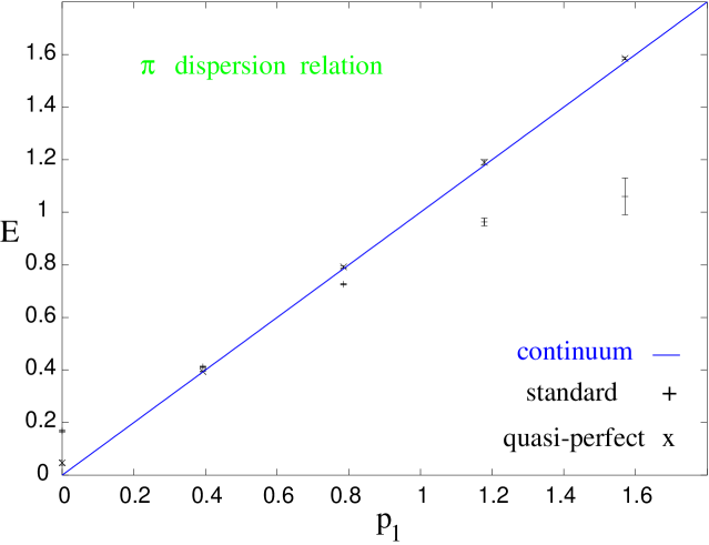
Figure 12: The dispersion relation for the pion with standard and the quasi-perfect action at $\beta=3$.

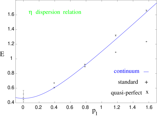
Figure 13: The dispersion relation for the $\eta$-particle with standard and the quasi-perfect action at $\beta=3$.

Finally, we show the $\beta$-dependence of the $\pi$- and $\eta$-mass in Figures 14 and 15. In the Schwinger model, asymptotic scaling for the $\eta$-mass is given by $m_{\eta}^{2}=2/\pi\beta$.

Figure 14: The $\beta$-dependence of $m_{\pi}$ with standard staggered fermions (squares) and quasi-perfect fermions, derived from $p_{1}=0$ (crosses) and $p_{1}=\pi/8$ (diamonds).

Figure 15: The $\beta$-dependence of $m_{\eta}$ with standard staggered fermions (squares) and quasi-perfect fermions, derived from $p_{1}=0$ (crosses) and $p_{1}=\pi/8$ (diamonds).

The nearly perfect dispersion relation of the quasi-perfect action makes it possible to derive the masses in a straightforward manner also from higher momenta, which leads to smaller errors for our data.

The $\eta$-mass should be equal to the decay mass $m_{gauge}$ of the plaquette correlation for zero spatial momentum. In our case, these are the most precise mass values. They can be extracted from a simple $\cosh$-fit. However, for reasons that we do not fully understand, $m_{gauge}$ does not follow the asymptotic scaling prediction as closely as $m_{\eta}$, see Figure 16.

Figure 16: The $\beta$-dependence of $m_{gauge}$ with standard staggered fermions (diamonds) and quasi-perfect fermions (crosses).

10 Conclusions

Spectral and thermodynamic results for free, truncated perfect staggered fermions have been presented before [24], but the improvement did not really reach a satisfactory level there. We now pushed that improvement significantly further, mainly thanks to the new blocking scheme, which we call partial decimation, but also with the help of a new truncation technique (mixed periodic boundary conditions). We now reached a level of excellent improvement, similar to the results for truncated perfect Wilson-type fermions.

We extended the construction of perfect actions to non-degenerate flavors, and we could preserve the same level of improvement after truncation also in that case. This is potentially important for the study of the decoupling of heavy flavors, or for QCD simulations with realistic quark masses.

At $m=0$, which is well described by staggered fermions, the PD scheme is optimally local if we just use a $\delta$ function RGT. This simplifies the relation to the continuum $n$-point functions, and numerical RGT steps, which could be performed for interacting theories (in the classical limit).

In $d=2$, we added an Abelian gauge field to this fermion along (selected) shortest lattice paths plus a “fat link”. In the latter, the weight $w$ of the staple term is optimized effectively, by minimizing the lowest eigenvalues of the fermion matrix, which led to $w=0.238$.

To simulate the 2-flavor Schwinger model, we applied a variant of the Hybrid Monte Carlo algorithm. It uses a simplified action in the identification of possible molecular dynamics steps, and the quasi-perfect action in the acceptance decision. In this way, we could avoid an increase in the computation effort proportional to the number of couplings.

As a vertex independent quantity, we measured the Fourier coefficients of the toron distribution, and we saw that even the free perfect action (without fat link) helps to move substantially closer to the continuum values.

Next we considered the dispersion relation of the “$\pi$” and “$\eta$” particle, and we extracted the masses $m_{\pi}$ and $m_{\eta}$ at varying $\beta$. We found a tiny pion mass down to $\beta$ $\stackrel{{\scriptstyle<}}{{\sim}}$ 1.5 which confirms an excellent scaling behavior of our quasi-perfect action, while $m_{\eta}(\beta)$ follows the asymptotic scaling very closely. A better scaling is the actual goal of the construction of improved actions, but it was observed before in other models that quasi-perfect actions also tend to improve the asymptotic scaling [13, 16].

These results, in particular the scaling is even better than the one obtained by using Wilson-type fermions with a classically perfect vertex function (parameterized by 123 independent couplings) [15]. This shows that truncated perfect free staggered fermions, which are suitably “gauged by hand”, can represent a highly improved, short-ranged action. This variant of a quasi-perfect improvement program is applicable and promising for QCD.

References

- [1] K. Wilson in “New Phenomena in Subnuclear Physics” ed. A. Zichichi, Plenum, New York (1975), part A, p. 69.
- [2] L. Susskind, Phys. Rev. D16 (1977) 3031.
- [3] Proceedings of LATTICE ’97, Nucl. Phys. B (Proc. Suppl.) 63 (1998).
- [4] K. Symanzik, Nucl. Phys. B226 (1983) 187; 205.
- [5] B. Sheikholeslami and R. Wohlert, Nucl. Phys. B259 (1985) 572.
- [6] M. Lüscher, S. Sint, R. Sommer, P. Weisz and U. Wolff, Nucl. Phys. B491 (1997) 323.
- [7] S. Naik, Nucl. Phys. B316 (1989) 238.
- [8] A. Peikert, B. Beinlich, A. Bicker, F. Karsch and E. Laermann, Nucl. Phys. B (Proc. Suppl.) 63 (1998) 895.
-
[9]
T. Blum et al.,
Phys. Rev. D55 (1997) 1133.
C. Bernard et al., Phys. Rev. D58 (1998) 014503.
See also J.-F. Lagaë and D. Sinclair, hep-lat/9806014. -
[10]
A. Patel and S. Sharpe, Nucl. Phys. B395 (1993)
701; B417 (1994) 307.
Y. Luo, Phys. Rev. D55 (1997) 353; Phys. Rev. D57 (1998) 265. -
[11]
K. Wilson and J. Kogut, Phys. Rep. C12 (1974) 75.
K. Wilson, Rev. Mod. Phys. 47 (1975) 773. - [12] P. Hasenfratz and F. Niedermayer, Nucl. Phys. B414 (1994) 785.
- [13] W. Bietenholz, E. Focht and U.-J. Wiese, Nucl. Phys. B436 (1995) 385.
-
[14]
M. Blatter, R. Burkhalter, P. Hasenfratz and F.
Niedermayer, Phys. Rev. D53 (1996) 923.
M. D’Elia, F. Farchioni and A. Papa, Phys. Rev. D55 (1997) 2274.
R. Burkhalter, Phys. Rev. D54 (1996) 4121. - [15] C. Lang and T. Pany, Nucl. Phys. B513 (1998) 645.
- [16] T. DeGrand, A. Hasenfratz, P. Hasenfratz and F. Niedermayer, Nucl. Phys. B454 (1995) 587; 615.
-
[17]
M. Blatter and F. Niedermayer,
Nucl. Phys. B 482 (1996) 286.
T. DeGrand, A. Hasenfratz and T. Kovacs, Talk presented at Yukawa International Seminar on Non-Perturbative QCD (Kyoto, 1997), hep-lat/9801037 and references therein.
E. Ilgenfritz, H. Markum, M. Müller-Preussker and S. Thurner, Phys. Rev. D58 (1998) 094502. -
[18]
W. Bietenholz and U.-J. Wiese, Phys. Lett. B378
(1996) 222.
F. Farchioni and V. Laliena, Nucl. Phys. B521 (1998) 337. - [19] W. Bietenholz and U.-J. Wiese, Nucl. Phys. B464 (1996) 319.
- [20] T. Kalkreuter, G. Mack and M. Speh, Int. J. Mod. Phys. C3 (1992) 121.
- [21] W. Bietenholz and U.-J. Wiese, Nucl. Phys. B (Proc. Suppl.) 34 (1994) 516.
-
[22]
G. Mai, “Ein Blockspin für Fermionen”,
diploma thesis, Hamburg (1989).
T. Kalkreuter, G. Mack, G. Palma and M. Speh, in “Lecture Notes in Physics” 409, eds. H. Gausterer and C. Lang, Springer, Berlin (1992) p. 205. - [23] H. Dilger, Nucl. Phys. B490 (1997) 331.
- [24] W. Bietenholz, R. Brower, S. Chandrasekharan and U.-J. Wiese, Nucl. Phys. B 495 (1997) 285.
- [25] J. Schwinger, Phys. Rev. 128 (1962) 2425.
- [26] I. Sachs and A. Wipf, Helv. Phys. Acta 65 (1992) 652.
- [27] H. Joos and S. Azakov, Helv. Phys. Acta 67 (1994) 723.
- [28] C. Gattringer and E. Seiler, Ann. Phys. 233 (1994) 97.
- [29] W. Bietenholz, R. Brower, S. Chandrasekharan and U.-J. Wiese, Nucl. Phys. B (Proc. Suppl.) 53 (1997) 921.
- [30] T. DeGrand for the MILC collaboration, Phys. Rev. D58 (1998) 094503.
- [31] K. Orginos et al., Nucl. Phys. B (Proc. Suppl.) 63 (1998) 904.
- [32] W. Bietenholz, N. Eicker, A. Frommer, Th. Lippert, B. Medeke, K. Schilling and G. Weuffen, hep-lat/9807013, to appear in Comp. Phys. Comm.
- [33] W. Bietenholz and H. Dilger, hep-lat/9810014, to appear in Nucl. Phys. B (Proc. Suppl.).
- [34] E. Kähler, Rend. Mat. Ser. V, 21 (1962) 425.
- [35] P. Becher and H. Joos, Z. Phys. C15 (1982) 343.
-
[36]
M. Göckeler and H. Joos, in “Progress in Gauge
Field Theory”, eds. G. ’t Hooft et al., Plenum, New York (1984), p. 247.
M. Golterman and J. Smit, Nucl. Phys. B278 (1986) 417.
G. Kilcup and S. Sharpe, Nucl. Phys. B283 (1987) 493. - [37] W. Bietenholz, Nucl. Phys. B (Proc. Suppl.) 63 (1998) 901.
-
[38]
M. Göckeler, Phys. Lett. B142 (1984) 197.
M. Golterman and J. Smit, Nucl. Phys. B245 (1984) 61. - [39] M. Lüscher, Comm. Math. Phys. 85 (1982) 39.
- [40] For a recent review, see Th. Lippert, hep-lat/9712019, published in Proc. of Workshop on Field Theoretical Tools in Polymer and Particle Physics (Wuppertal 1997), Springer, Lecture Notes in Physics 508, ed. H. Meyer-Ortmanns and A. Klümper, p.122.
- [41] B. Berg and Th. Neuhaus, Phys. Lett. B267 (1991) 249; Phys. Rev. Lett. 68 (1992) 9.
- [42] H. Dilger, Nucl. Phys. B434 (1995) 321.
- [43] R. Frezzotti and K. Jansen, Phys. Lett. B402 (1997) 328; hep-lat/9808011; hep-lat/9808038.
- [44] H. Dilger, Int. J. Mod. Phys. C6 (1995) 123.
- [45] Ph. de Forcrand and J. Hetrick, Nucl. Phys. B (Proc. Suppl.) 42 (1995) 861.
- [46] W. Bietenholz, hep-lat/9803023, to appear in Europ. Phys. J. C.